Extended metric validation of a semi-physical Space Weather Modeling Framework conductance model on field-aligned current estimations

In this study, a detailed metric survey on the “Galaxy 15” (April 2010) space weather event is conducted to validate MAGNetosphere–Ionosphere–Thermosphere (MAGNIT), a semi-physical auroral ionospheric conductance model characterizing four precipitation sources, against AMPERE measurements via field-aligned current (FAC) characteristics. As part of this study, the comparative performance of three ionosphere electrodynamic specifications involving auroral conductance models, MAGNIT, Ridley Legacy Model (RLM) (empirical), and Conductance Model for Extreme Events (CMEE) (empirical), within the Space Weather Modeling Framework (SWMF), is demonstrated. Overall, MAGNIT exhibits marginally improved predictions; root mean square error values in upward and downward FACs of MAGNIT predictions compared to AMPERE data are smaller than those of CMEE and Ridley Ionosphere Model (RIM) by $\sim$12.7% and $\sim$6.24% before the storm, $\sim$4.52% and $\sim$2.13% better during the main phase, $\sim$1.98% and $\sim$1.27% worse during the second minimum, and better by $\sim$1.84% and $\sim$1.49% by the beginning of the recovery, respectively. In all three model configurations, the dusk and night magnetic local time (MLT) sectors over-predict throughout the storm, while the day and dawn MLT sectors under-predict in response to interplanetary magnetic field (IMF) conditions. In addition to accuracy and bias, similar results and conclusions are drawn from additional metrics, including in the categories of correlation, precision, extremes, and skill, and recommendations are made for the best-performing model configuration in each metric category. Visual data–model comparisons conducted by studying the FAC location and latitude/MLT spread throughout various phases of the storm suggest that the spatial extent of the FACs is captured relatively well in the night-side auroral oval, unlike in the day-side oval. The spread in latitude of the FACs matches that in the previous literature on other model performances. This information on auroral precipitation sources and their weight on FACs, along with metrics from model–data comparisons, can be used to modify MAGNIT settings to optimize SWMF model performance.

1 Introduction

Field-aligned currents (FACs) play a major role in ionosphere–magnetosphere coupling as a significant process through which energy and momentum are exchanged between the two systems (Kamide, 1982; Saflekos et al., 1982; Lysak, 1990). Today, the space physics community’s understanding of FACs includes the mapping extent and locations within the magnetosphere and ionosphere and the energy content relationship from solar wind driving. Major components of FACs are split into regions 0, 1, and 2 and related to one another through the Hall and Pedersen currents (Iijima and Potemra, 1976). Region 1 and 2 FACs tie the ionosphere with the magnetopause or plasma sheet and partial ring current, respectively, with the high-latitude region 1 FACs flowing inward on the dawn side and outward on the dusk side and the region 2 FACs having an opposite flow pattern at slightly lower latitudes. In response to the imposed electric fields in the ionosphere, the Hall and Pedersen currents are generated (Le et al., 2010). With northward interplanetary magnetic field (IMF) driving, region 0 or day-side cusp currents appear just pole-ward of the region 1 FACs (Watanabe et al., 1998).

FACs are critical to understanding numerous applications, including predictions of aurora generation (Knight, 1973) and (geomagnetically induced) current intensities. Models are diverse, some directly¹ calculating FACs (for example, transient features (Gombosi and Nagy, 1989), while others use satellite data to recreate FACs (for example, Iridium [Anderson et al., 2000], Dynamics Explorer 2 [Weimer, 2001], Swarm [Ritter et al., 2013], and combinations of various satellites and/or ground-based measurements [He et al., 2012; Edwards et al., 2019]). In the general prediction of space weather, FACs are calculated as the curl of the magnetic field and serve as precursors to calculating other related quantities in ionosphere–magnetosphere coupling, such as auroral precipitation (examples of IM-coupled models: LFM [Zhang et al., 2000], Open GGCM [Raeder et al., 2008], and Space Weather Modeling Framework (SWMF) [Toth et al., 2005]). This makes FACs an extremely useful quantity for validating the flexible performance of models and modeling frameworks that, in practical applications, must predict values different from their design purposes (Pulkkinen et al., 2013)².

Space weather model validation efforts often focus on basic statistical comparisons against in situ point observations. Many of these studies constrain their model validation to the performance of a limited metric, typically measuring its ability to replicate and forecast. Some examples include the following:

•Glocer et al. (2016) used the Heidke Skill Score (HSS) and a newly defined distribution metric to evaluate NOAA/Space Weather Prediction Center (SWPC) modeling of the auroral K-index.

•Lane et al. (2014) used prediction efficiency (PE) to describe the OVATION Prime model, the Hardy 1991 Kp-based model, and a coupled SWMF ring-current model against the Defense Meteorological Satellite Program (DMSP) energy flux.

•Mukhopadhyay et al. (2022b) used median absolute percentage error (MAPE) and exclusion parameter (EP) to validate the MAGNetosphere-Ionosphere-Thermosphere (MAGNIT) model for the first time, against the SWMF-Ridley Legacy model (RLM), SWMF-Conductance Model for Extreme Events (CMEE), and DMSP.

This, however, does not fully reveal information that could lead to improvements in model performance or understanding of the underlying physics (Liemohn et al., 2021). For example, the reveal of a bias helps provide context for model usage—whether the model is over-predicting or under-predicting in various scenarios is useful for the user. A combination of studying standard deviations to understand the spread of values and extremes describes the entirety of a distribution and can be targeted when modeling extreme events and values. Investigating model performance with various errors expands the storyline to allow for a variety of use cases (Liemohn et al., 2021).

This work adds to the validation effort of the MAGNIT model coupled within the SWMF, where MAGNIT is selected as the conductance solver within the Ridley Ionosphere Model (RIM) to constitute the ionosphere electrodynamics (IE) component. Unlike previous empirical models of ionospheric conductance within RIM based on ionosphere electrodynamic heatmaps, the new, semi-physical model is capable of identifying and calculating four auroral precipitation sources—electron and ion diffuse, monoenergetic, and broadband. Additional details are given in the Methodology section (Mukhopadhyay, 2021; Mukhopadhyay et al., 2022b). This validation effort covered over 11 metrics among 5 categories³ to suggest a full understanding of how the model can predict FACs, a quantity independent of model development.

2 Methodology

For the statistical comparison, the performance of three SWMF model configurations with differing IE components over the 5–7 April 2010 “Galaxy 15” event was investigated against AMPERE data. This section provides details on the event (Subsection 2.1), models (Subsection 2.2), and statistical methods (Subsection 2.3).

2.1 Event Information

The Galaxy 15 storm characteristics are shown in Figure 1. The CME-shock-driven space weather event is named after the satellite it damaged and has been extensively studied for having an extreme expansion phase and resulting dipolarization (Loto’aniu et al., 2015; Nishimura et al., 2020; Sergeev et al., 2011). For the purposes of this study, the event is split into four different epochs—“before the storm” (Epoch 0: April 5, 00 UT–8:24 UT) prior to sudden commencement, “during the main phase” (Epoch 1: 8:24–10:48 UT), “during the second minimum” (Epoch 2: 10:48–17:36 UT), and “during recovery” (Epoch 3: April 5, 17:36 UT–April 6, 00:00 UT; this is not the full extent of the recovery period). Epoch 1 is characterized by negative IMF Bz and positive IMF By, containing the first peak in activity. Epoch 2 is characterized by positive IMF Bz and negative IMF By, corresponding to a second peak in activity. The different epochs are labeled in Figure 1. The epochs were chosen based on similarities in the Galaxy 15 storm characteristics (see Section 3, Results; Table 2). As a highly active event, the Galaxy 15 storm given in Figure 1 illustrates the progression of ionospheric conductance as the storm interacts with the magnetosphere. At sudden commencement in Epoch 1, the day-side magnetosphere experiences a strong compression evident with the positive Sym-H. While conductance in the day-side ionosphere typically arises from solar EUV flux, the strong compression causes the Chapman–Ferraro current to come close to the planet, temporarily increasing precipitation from the magnetosphere into the cusp on the day-side. As the storm progresses, reconnection and activity in the tail propagate planet-ward, leading to increased auroral precipitation, conductance, and FAC activity on the night-side.

Figure 1

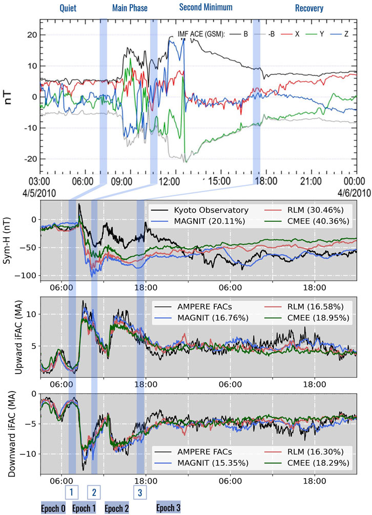
Figure 1. Galaxy 15 storm event characteristics are shown split into four different epochs, as explained in Section 2.1. The top subplot describes ACE spacecraft magnetic field data of the storm, obtained from Anderson et al. (2017). The bottom three subplots show observed AMPERE data in black and output predicted from SWMF model configurations described in Section 2.2 for the Sym-H index and integrated upward and downward field-aligned currents (iFACs) (Mukhopadhyay et al., 2022b). Note that the three model configurations (MAGNIT, CMEE, and RLM) generate Sym-H and downward and upward FACs in strong agreement with AMPERE. Figures have been obtained from Anderson et al. (2017) and Mukhopadhyay et al. (2022b) and annotated by the authors.

The Galaxy 15 storm was recorded by a number of spacecraft and ground observations, including data from the AMPERE dataset collected from the Iridium satellite constellation⁴ (Waters et al., 2001; Anderson et al., 2021; 2002; Waters et al., 2020). The 66 polar inclination spacecraft spread along 6 evenly distributed meridian circles across the globe gathered magnetic field perturbations over 24 h (April 5, 00:00 UT–April 6, 00:00 UT) in LEO, at an altitude of $\sim$780 km. In this study, the calculated radial current, also interpreted as FAC, was used as the comparator—the quantity is significant in research value and was not a quantity used to train any of the SWMF model configurations. In AMPERE, up and down FACs are derived by identifying and categorizing magnetic field variations measured by the magnetometers of the Iridium satellites and are then used in combination to recreate a map (Anderson et al., 2000; Waters et al., 2001). In this analysis, observation–model data comparisons are made only along the six orbit satellite tracks every 2 min to match the temporal resolution of AMPERE values and decrease the sources of uncertainty. As with any satellite measurement, instrument and measurement resolution and uncertainties limit the capability of the observation to be a perfect “ground truth.” Because the “observation” radial current in AMPERE is a derived quantity from measured electromagnetic parameters, in this paper, we refer to them interchangeably as “observationally derived estimates.”

The FAC patterns are studied to probe questions about the spatial performance of the various SWMF model configurations within the auroral oval region. While the entire auroral oval is viewed as a whole, data points were also categorized into four spatial regions defined by 6-h increments as “dawn” (03–09 MLT), “day” (09–15 MLT), “dusk” (15–21 MLT), and “night” (21–03 MLT). Investigating various SWMF configuration performances grouped by time (storm progression) and space (magnetic local times) provides the opportunity to understand the overall and localized uncertainty features in FAC predictions.

2.2 Model configuration

The geospace version of the SWMF⁴ currently used at NOAA-SWPC for real-time space weather prediction (Pulkkinen et al., 2021) comprises a multitude of physics domains distributed using numerical models (Tóth et al., 2012) that describe plasma interactions across the global magnetosphere (GM), inner magnetosphere (IM), and (IE) regions. An example of a publicly available configuration⁵ is the BATS-R-US global magneto-hydrodynamics (MHD) model (Powell et al., 1999) (GM), the Rice Convection Model (RCM) ring current (Toffoletto et al., 2003; Zeeuw et al., 2004) model (IM), and the RIM Poisson solver (Ridley et al., 2004) (IE). This study uses data originally produced by Mukhopadhyay et al. (2022b), which include details on the limitations of different domains. The auroral conductance specified by default in RIM is referred to in this paper as the RLM (Ridley et al., 2004). The two other model configurations switch auroral conductance estimations from RLM to CMEE and MAGNIT, as detailed below. Figure 2 visualizes the relationship between the modules of the SWMF, specifically GM (BATS-R-US), IM (RCM), and IE (RIM with the RLM or CMEE or MAGNIT), and how they are coupled to one another within the framework. The connecting processes shown in Figure 2 are described in more detail in the following paragraphs.

Figure 2

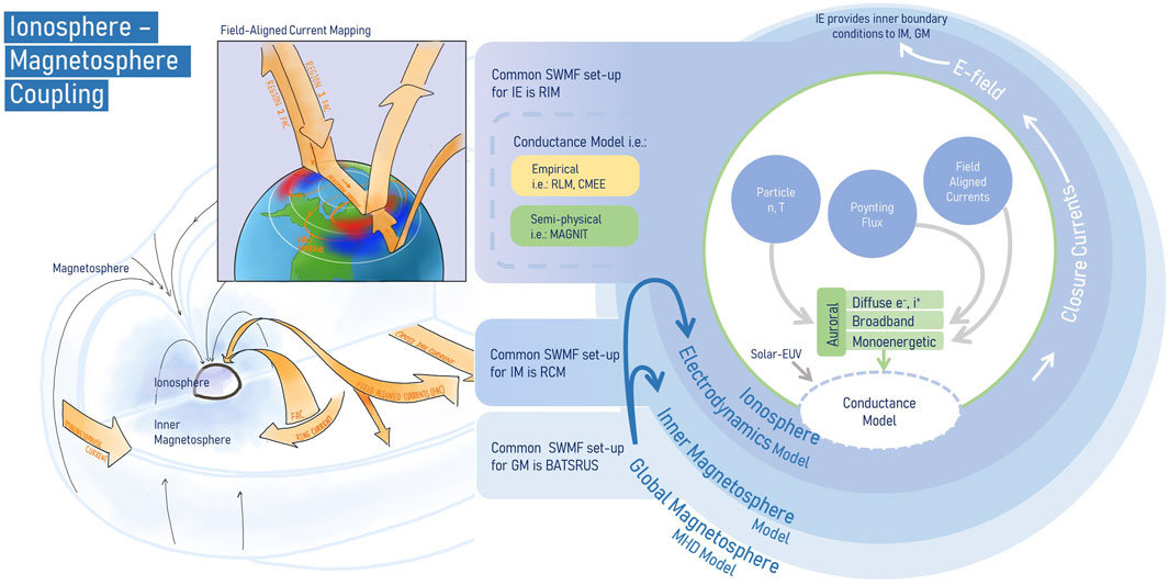
Figure 2. The coupling relationship between various geospace regimes (GM, IM, and IE) in the SWMF is shown. Each regime provides boundary conditions for the others. For ionospheric conductance specified by empirical models SWMF-CMEE and SWMF-RLM, auroral precipitation sources are grouped as a singular quantity, distinguished individually only in the semi-physical model SWMF-MAGNIT.

Both RLM and CMEE (Mukhopadhyay et al., 2020) are empirical models based on data from assimilative mapping of ionospheric electrodynamics (AMIE) (Kihn and Ridley, 2005); RLM is trained on the relatively quiet month of January 1997, while CMEE is trained on the entire highly active year of 2003 in an effort to include extreme events. The conductance values are related to FACs via a weighted inverse exponential relationship (see Mukhopadhyay et al., 2022b), which are used in the IE model and, consequently, in the GM model’s MHD quantities, feeding back as boundary conditions between the domains. MAGNIT is a semi-physical model that calculates electron and ion diffuse, monoenergetic, and broadband auroral precipitation based on MHD quantities near the inner boundary. The auroral precipitation sources are combined with a root-sum-square formula and used to calculate conductance, which then feeds into the IE and GM model MHD quantities. Thus, while SWMF-RLM and SWMF-CMEE only use MHD-produced FAC characteristics, SWMF-MAGNIT uses MHD electric and magnetic field values, densities, and pressures in addition to FACs. This applies to SWMF-MAGNIT diffuse and broadband auroral precipitation, but for discrete monoenergetic auroral precipitation, the Knight–Fridman–Lemaire relationship is used to estimate values. The auroral precipitation and conductance in the three different SWMF model configurations are supplemented with EUV flux in the larger RIM.

The Galaxy 15 event was run with no preconditioning. BATS-R-US was used as a semi-relativistic single-fluid MHD solver (Boris, 1970) over the domain X $+32R_E$ to $-224R_E$ and Y and Z $-128R_E$ to $+128R_E$, with the Hi-SWPC grid resolution (Haiducek et al., 2017; Mukhopadhyay et al., 2020). Flux-tube volume information was passed to RCM, which solved for bounce-average particle distributions and returned MHD pressure and density values to BATS-R-US. Although RCM is capable of passing particle energy information to IE models, that option was not used (Mukhopadhyay et al., 2022a). In addition to MHD pressure and density values, BATS-R-US also mapped the FACs from $3.5R_E$, near its $2.5R_E$ inner boundary to the IE models at an ionospheric altitude of 110 km. The IE with a grid resolution consisting of $91\times 181$ cells, with a $2°$ cadence in both latitude and longitude, provided the ionospheric potential to be used as inner-boundary conditions for BATS-R-US and RCM. The various models were coupled to one another at 5- or 10-s cadences, and FAC values were recorded at a 1-min temporal resolution.

2.3 Statistical methods

In addition to visual and numerical representations of FAC patterns to describe the error of the three model configurations in replicating AMPERE data, error characteristics were extended to include several numerical metrics. In this study, metrics describing accuracy, bias, precision, association, and extremes are explored (Liemohn et al., 2021). Descriptions and examples of metrics categories addressed in this analysis are outlined in Table 1, including their units or lack thereof. To consolidate findings, some metrics are excluded due to their similarities to already discussed quantities (for example, root mean square error [RMSE] in lieu of the mean square error and mean absolute error), while others are excluded due to their tendency to approach infinity and therefore are not useful (for example, symmetric signed percentage bias [SSPB] includes weighting by observed data points; in the AMPERE data, near-0 FAC values are included that cause some SSPB points with low measured FACs to have excessively large values).

Table 1

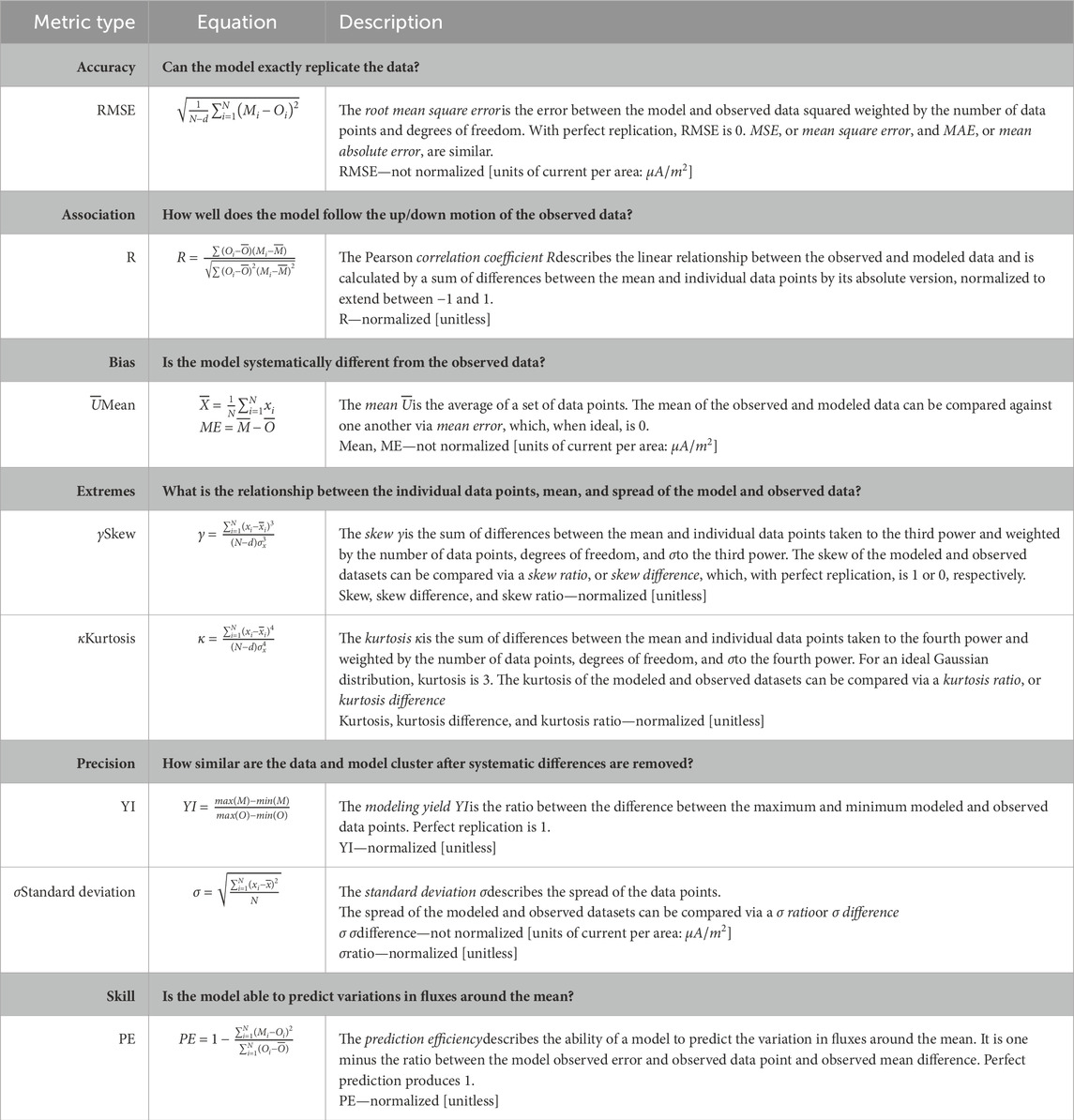
Table 1. Summary of metric categories utilized in this study, inspired by recommendations made in Liemohn et al. (2021).

The traditional standard error on the conductance and radial current representing FACs produced by the model and reported in AMPERE is an unanswered task across the field and remains unsolved here. Similar to other in situ and remote observations, the standard radial current data available for the AMPERE repository⁶ do not provide uncertainties in measurement positions or calculated data products. As data increasingly become open source, uncertainties related to measurement positions relative to various coordinate systems, instrument uncertainties, and the effects of interpolations and noise filtering should be propagated to establish a central error margin. Like other dynamic space environment models, predicting conductance and FACs in the models available in the SWMF is a complex, multi-step process with uncertainties at each stage. For MAGNIT, the first step involves deriving estimated energy flux and average energies from MHD quantities. Although this is a challenge due to the assumption of a highly kinetic process within a hydrodynamic model that lacks particle representation, it is well-documented by Mukhopadhyay et al. (2022b) with comparisons to other models. For RLM and CMEE, the initial error originates from AMIE’s use of ground-based magnetometer data and empirical relations to derive conductance and FACs; the uncertainties associated with conductance in these models, compared to AMIE, are detailed by Mukhopadhyay et al. (2020) for specific locations, although a global-scale analysis remains unaddressed. The second layer of uncertainty arises in MAGNIT, CMEE, and RLM from computing conductance by fluxes or vice versa. The uncertainties related to the Robinson relationship are well known, and despite its issues, is used widely (Liemohn, 2020). The third and most critical level of uncertainty is in computing ionospheric electrodynamics from conductance values, which is documented in part in numerous studies (Liemohn et al., 2006; Pulkkinen et al., 2013; Mukhopadhyay, 2021). This paper further explores metrics related to these ionospheric electrodynamic parameters.

Because metrics are designed to test a specific characteristic, their relative “goodness” varies. To account for uncertainty on top of each error metric, a bootstrap test was conducted using 10,000 re-samplings with replacements until the distribution of uncertainty appeared visually Gaussian. The standard error on each error metric was found based on the spread of the metric values from these 10,000 bootstrap re-samplings. These bootstrap standard errors are given in Table 3. Despite its name, it is the standard deviation of the bootstrap distribution and, thus, the standard error on each metric. For most metrics, the proximity of the value to a central desired quantity (for example, difference ratios) shows the preferential suitability of that value as “good.” Some metrics like RMSE are always positive, whereas other metrics like correlation coefficient (R) contain desirable characteristics when positive and undesirable characteristics when negative.

As described in Event Information (Subsection 2.1) and Model Configuration (Subsection 2.2), data were grouped by epoch, model, and magnetic local time. The “best” and “worst” values for each metric category and a list of standard errors are given in Tables 2, 3.

Table 2

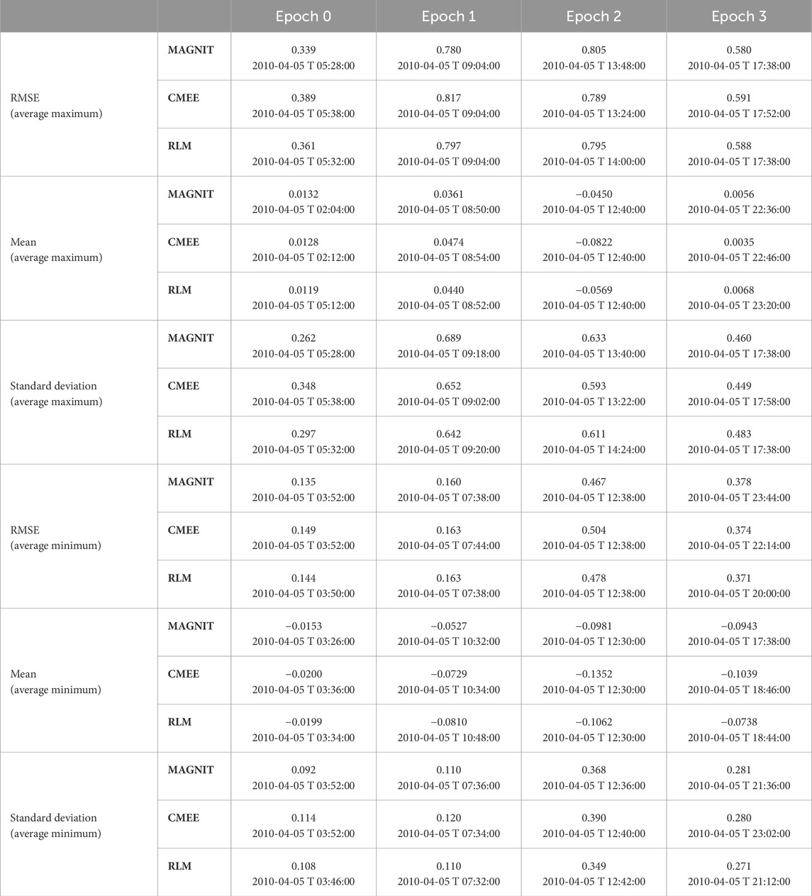
Table 2. Peak maximum and minimum metric values for each epoch are recorded for RMSE, mean, and standard deviation metrics. Values have been averaged over 10 min, and the time recorded is at the center. Note similarities in each epoch across different SWMF configurations and metrics, suggesting that the limiting bounds of each epoch are acceptable. For RMSE, the best and worst scores within each epoch have been colored green and red, respectively.

Table 3

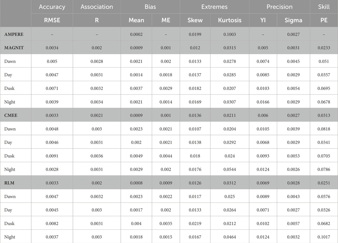
Table 3. The uncertainty of each metric calculated via a bootstrap test, as explained in Section 2.3, is shown here, truncated after four places. The uncertainties of each metric are, for the most part, much smaller than the metric values given in Figures 4, 6.

3 Results

In this section, we characterize the performance of the modeled results against measurements from the AMPERE dataset, highlighting select metrics in each category to derive information on model performance by MLT sector over time. Examples of the field-aligned currents constructed by the various model configurations are shown in Figure 3, along with AMPERE FACs at three event times. Table 2 provides a description of these event times that separate four epochs based on similar storm progression and model performance. The three time stamps selected are 1) before the sudden commencement of the storm, 2) during the main pulse, and 3) in the recovery phase of the storm. In Figure 3, both the upward and downward FACs are plotted in the Northern polar region, showing the North Pole at the origin and extending to latitude $60°$ at the outer edge; MLT noon toward the top of the page; and midnight toward the bottom of the page. The models resemble one another with similar FAC patterns, and the magnitude of upward and downward FACs is representative of magnitudes observed in AMPERE (Figure 1). The modeled FACs appear wider in latitude than the observed currents and are not identical in MLT. Upward and downward FAC structures in AMPERE are consistent with the models but have notably different fine structures. We note that the higher-order harmonics observed by AMPERE in the mid and high latitudes can be smoothed out with a low-pass filter, while lower-latitude fine structures may be a product of spacecraft instrument noise. Before major storm activity, models have little difference compared to AMPERE’s observationally derived estimates, and as the activity progresses, the models tend to over-predict downward FAC values in the day/dawn sector. The models are similar to observed data in the dusk/night sector. This evolution is discussed in more detail in subsequent sections. It is important to fully understand various model performances over time and at various MLTs to drive future model improvement and the best practices for model validation. Supporting products include graphical investigations (Figures 4, 6), numerical analysis (Tables 1–3), and numerical comparisons (Figures 5, 7, 8). The following subsections are organized by metric category and further explain trends and characteristics observed in the figures outlined.

Figure 3

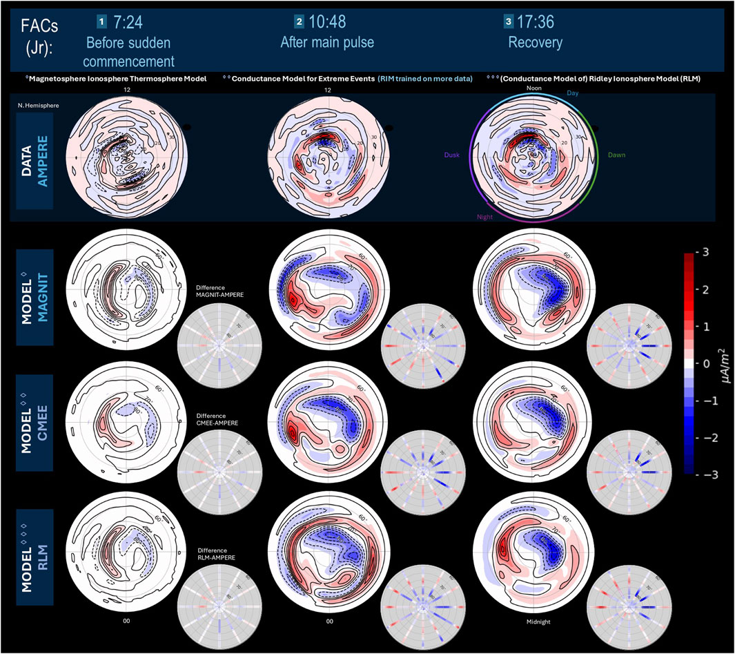
Figure 3. FAC patterns as measured by AMPERE and predicted by the SWMF-MAGNIT/CMEE/RLM in the Northern Hemisphere are shown for select times of the Galaxy 15 storm. The large circular plots show upward (red) and downward (blue) FACs. The smaller circular plots show direct differences between the modeled and AMPERE data across Iridium satellite tracks; red positive values can be interpreted as an over-prediction of upward FAC values or an under-prediction of downward FAC values, while blue negative values are an under-prediction of upward FAC values or an over-prediction of downward FAC values.

Figure 4

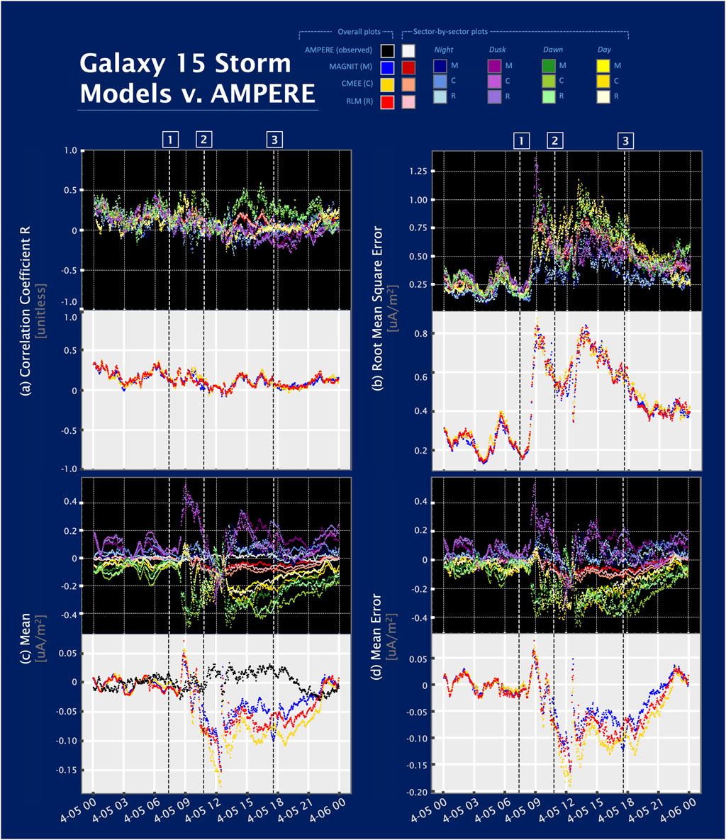
Figure 4. The performance of various model configurations grouped by MLTs across the storm is shown for (A) the association metric R (correlation coefficient; Section 3.2), (B) the accuracy metric RMSE (root mean square error; Section 3.1), (C) the general quantity Mean, and (D) the bias metric Mean Error (C,D) (Section 3.3 (Section 3.3.1, Section 3.3.2)). Deviation from nominal metric behavior is consistent across (B–D) at the same time following the beginning of the storm. Note that for the mean error, upward and downward FACs add a layer of complexity, while for the correlation coefficient and root mean square error, only magnitudes of the FACs are utilized. The standard error on each metric is given in Table 3 and is not plotted on their respective graphs because of its small size, which was not clearly visible.

3.1 Accuracy: RMSE

Accuracy is the most recognizable term when designing a model to replicate exact observations. The RMSE is a common metric of accuracy, and in this study, it measures the pure difference in FAC values between model and observed data points. Figure 4 shows a summary of four statistics comparing AMPERE data to the output of each conductance model over the course of the full geomagnetic storm. Each subplot is further divided into a top panel with a black background, showing results grouped by MLT sector, and a bottom panel with a light gray background showing global results. The accuracy metric RMSE is plotted in Figure 4B. The overall performance of the three model configurations is comparable to one another, and errors increase in response to IMF fluctuations, peaking at $\sim 9$ UT and $\sim 10$ UT, following the sudden increase/decrease in IMF $B_y$ and decrease/increase in IMF $B_z$, respectively. The RMSE is larger than 1 only briefly at the beginning of storm activity; for the rest of the storm, the errors in FACs are less than the FAC magnitudes.

MAGNIT has the lowest RMSE value throughout the storm and, thus, slightly better accuracy. The average and the best values of RMSE by epoch are listed in Table 2. RMSE values of MAGNIT are initially smaller than those for CMEE and RLM by $\sim$12.7% and $\sim$6.24% before the storm, decrease to differences of $\sim$4.52% and $\sim$2.13% during the main phase, become worse by $\sim$1.98% and $\sim$1.27% during the second minimum, and become better again by $\sim$1.84% and $\sim$1.49% by the beginning of the recovery phase. Data comparison in various MLT sectors also follows the same pattern, with the least error contributed by the night sector in all three model configurations. Prior to the sudden commencement in Epoch 1, errors were slightly larger in the dawn and dusk sectors. With the sudden and extreme increases in RMSE after sudden commencement and again after the main pulse, the largest contributors become day and dawn. A clear return to pre-storm values of the RMSE is observed during recovery.

The RMSE and accuracy do not describe how or why the model data deviate from observed values. Thus, how the models are biased and how the data distribution is shaped must also be investigated.

3.2 Association: correlation coefficient

The correlation coefficient, R, is often used as the singular metric to describe performance and is a proxy for the linear relationship between the model and observed data. In essence, it describes the ability of the model to replicate the motions of the measured data. Figure 4A shows the correlation coefficient over the course of the storm. As shown in Figure 4A and supported by statistics on the metric data (average and best values are listed in Table 2), the association performance of the three model configurations is mostly indistinguishable from one another. The values are far from the ideal model–data comparison, and the association has a slightly downward trend as the storm progresses. Despite this, the standard error associated with R is less than 5% of the R-value; however, in 7 of the 60 model/MLT sector and overall auroral oval/epoch combinations, the standard error on R increases to more than 10%. The most severe uncertainties are common during Epoch 2 and in the night sectors. FAC data in the dawn sector have a better association than other MLT sectors and consistently remain positive, while the dusk sector has a negative correlation during the second minimum (Epoch 2) and continues into recovery. In Epoch 3, this negative correlation is less severe in MAGNIT than in RLM or CMEE. Throughout the storm, the association of all MLT sectors and the globally averaged FACs in the auroral oval oscillates at approximately 0 $\mu A/m^2$, having neither a strong positive nor negative correlation. Because of the massive amount of data points and the low FAC values across a wide map, this is expected.

The t-test is a statistical test that reveals whether a difference in scores of two datasets, in this case, the R-value, is due to random chance. The null hypothesis of the test is that the score of the two datasets has the same mean, and $\alpha$ (significance level) is the probability of rejecting the null hypothesis when it is true. The p-value measures the statistical significance of the result, and for a given confidence threshold, it accepts the null hypothesis if $p_{\text{calculated}}>p_{\alpha }$ and rejects it if $p_{\text{calculated}}<p_{\alpha }$. For a 95% confidence level, the critical p-value $(p_{\alpha })$ is 0.05, which is the maximum requirement for the score to be statistically significant such that the R-value did not arise from chance. The p-values of the various configurations suggest that R is only comparable with AMPERE FAC data occasionally; model and MLT sectors comparable in R with observations are listed below, supported by the calculated p-values documented in parenthesis:

• MAGNIT and RLM Day (Day M/C/R: 0.167$\cdot 10^{-2}$/0.504/0.013);

• MAGNIT and RLM Dawn (Dawn M/C/R: 0.111$\cdot 10^{-2}$/0.711/0.441$\cdot 10^{-2}$);

• MAGNIT and CMEE Dusk (Dusk M/C/R: 0.102$\cdot 10^{-5}$/0.653$\cdot 10^{-4}$/0.418);

• None of MAGNIT/CMEE/RIM Night had an acceptable p-value (Night M/C/R: 0.102/0.289/0.547).

Although MAGNIT R-values reject the null hypothesis in the t-test, while CMEE and RLM are less likely to do so, this provides little suggestion of a trend in association.

3.3 Bias: mean and mean error

Bias describes systemic differences in the data–model comparisons. In the overall performance of the models, the three configurations tend to slightly under-predict during the activity of the storm. When examining the mean error, CMEE provides the best performance in terms of the globally averaged modeled and observed FACs. However, MAGNIT shows strong potential in explaining underlying physics as it has the best performance when comparing the modeled MLT sectors with the observed average of the auroral region. The bias is not consistent as the storm progresses through different epochs, and varying under-prediction and over-prediction patterns are observed in some of the MLT groupings across the models.

3.3.1 Mean

Figure 4C shows the spatial mean of current density over the entire high-latitude region (above $50°$) at each time stamp. The average spatial mean of the AMPERE data throughout the storm is near $0\mu A/m^2$, including both upward and downward FACs. In Epoch 0 pre-storm, AMPERE, CMEE, RLM, and MAGNIT values are similarly near 0 but deviate in Epoch 1. The models sharply over-predict at $\sim 9$ UT, following a sudden increase in $B_y$ and decrease in $B_z$. They then begin to show a more consistent under-prediction around 10 UT, where $B_y$ decreases to negative values and $B_z$ increases to positive values. This under-prediction continues into Epoch 2, and in general, observed data are most closely replicated by MAGNIT and then by RLM and CMEE, respectively. There are two exceptions: near $\sim$12:30 UT, corresponding to the sudden decrease in $B_z$ back to 0, where the mean of observed AMPERE data is briefly negative, and thus, the low mean values of the three model configurations are insignificant at that time. The other exception is the temporary peak under-prediction by MAGNIT at the border between epochs 2 and 3. As the environment begins to recover in Epoch 3, the models return to an average mean of 0, similar to AMPERE data.

The typical mean values of the MLT sectors for the three models are similar to those of the overall auroral oval but with magnitudes cut in half. Dusk and night sectors tend to over-predict, while day and dawn sectors under-predict. An exception occurs at $\sim 12$ UT, while $B_z$ reaches its maximum positive values. The over-prediction of FACs in the dusk sector is mirrored by an under-prediction in dawn during Epoch 1, day in Epoch 2, and dawn again during Epoch 3. Although all model/MLT sector combinations return to nominal performance during the storm recovery phase, MAGNIT dusk and CMEE dawn are the most gradual, transitioning from over-predicting/under-predicting, respectively. Throughout the storm, the night sectors across all three models have the least bias against the AMPERE data.

3.3.2 Mean error

Figure 4D shows the mean error (ME) over the course of the whole geomagnetic storm, both divided by MLT sector (top, black background) and globally (bottom, gray background). The ME follows a similar trend to the other metrics, with maximum error near the time of sudden commencement. Figure 5 provides additional insight into the biases of various model/MLT sector combinations by comparing the mean error of the various models. Numbers characterizing bias performance for each model/MLT sector combination are shown for the four epochs by defining an “ideal point” envelope centered around 0 bias with a width of 10 standard errors of bias (not to be confused with the standard errors of the modeled and observed FACs). Positive mean error values can be interpreted as both an overestimation of upward FACs and an underestimation of downward FACs. Similarly, negative mean error values can be interpreted as an underestimation of upward FACs or an overestimation of downward FACs. Figure 5B shows the percentage of ideal points within each epoch. Figure 5C shows the relative number of ideal points in the same MLT sector and time, such that there is a top-performing, standard, and lowest-performing conductance model shown in green, yellow, and red for each spatial and temporal combination, respectively.

Figure 5

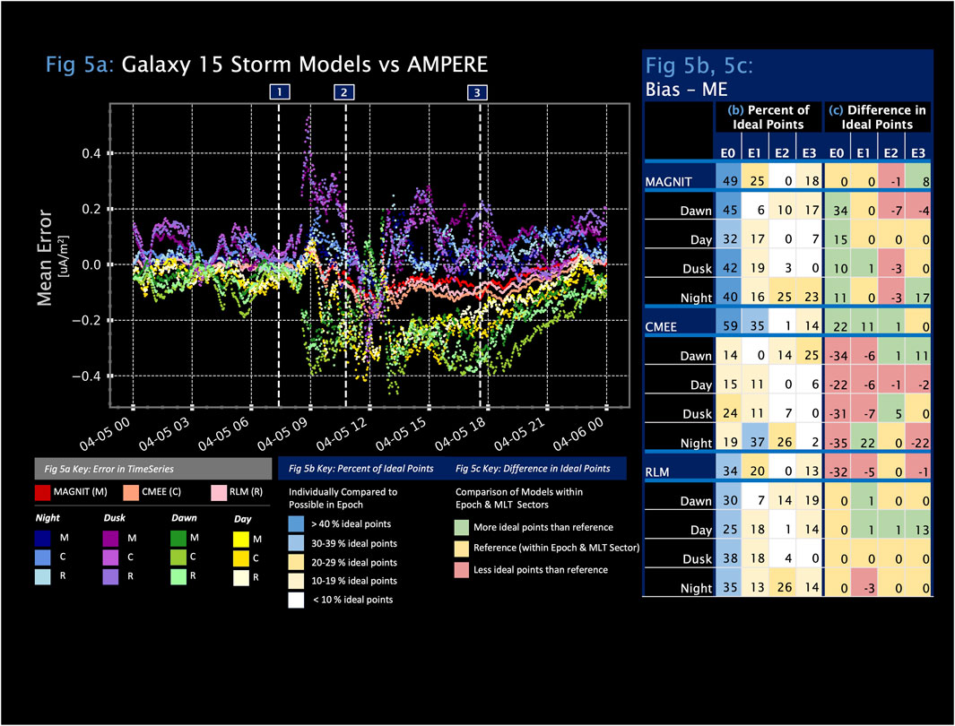
Figure 5. (A) Mean error (ME) values throughout the storm. Positive/negative ME values arise from an over/underestimation of upward FACs or an under/overestimation of downward FAC values. (B) Percentage of ideal points for each model configuration, MLT grouping, and epoch. (C) Relative number of ideal points for each MLT grouping and epoch combination to compare the performance of various model configurations. For example, in Epoch 1 dawn (C), the best performer in the overall polar region is colored green (RLM by one data point), while the medium performer is colored yellow (MAGNIT), and the worst performer is colored red (CMEE by six points). Ideal points are defined to be within $\pm 10\text{\hspace{0.17em}Standard\hspace{0.17em}Errors\hspace{0.17em}}\left(\text{SE}\right)$ of the ideal value of 0 bias and are, therefore, data points with very little over- or underestimation. Additional explanation is provided in Section 3.3.

The bias in MAGNIT, CMEE, and RLM increases throughout the storm; hence, the percent of ideal points is generally the largest during Epoch 0. A minimum percent of ideal points is recorded during the storm’s sudden commencement in Epoch 2, after which in Epoch 3 an improvement to levels of approximately half of Epoch 1 is made. Analysis of the overall polar region shows that CMEE begins with more than half (59%) of points considered ideal, followed by MAGNIT at nearly half (49%) of points and RLM at 34%. The trend continues through Epoch 1 (CMEE 35%, MAGNIT 25%, and RLM 20 %) and Epoch 2 (CMEE 1% and MAGNIT and RLM 0%); however, during Epoch 3, CMEE and RLM do not recover as quickly in regaining ideal points (14% and 13%, respectively) as MAGNIT (18%).

When investigating MLT sector performance, CMEE is no longer the highest-performing conductance model as it was globally. MAGNIT has significantly more ideal points before the storm in Epoch 0, followed by RLM (average difference of 7.75% versus MAGNIT) and CMEE (21.75% difference versus MAGNIT). As the storm continues, the three models become comparable to one another as the difference in the number of ideal points decreases. The night sector consistently has more ideal points than any other sectors in all three model configurations, and while the night and dawn sector recovers significantly during the storm recovery phase, dusk does not recover at all.

3.4 Precision: modeling yield and standard deviation ratio and difference

Precision explores the characteristic shape of the data population. Similar to the bias metric, the performance of the overall northern hemisphere is slightly higher in CMEE run than that in the RLM and MAGNIT runs but overtaken by MAGNIT when investigating MLT sectors. The models have spreads and population curves similar to observed AMPERE data throughout the storm, with individual trends by models and MLT sectors detailed below. Figure 6 is styled similarly to Figure 4 but shows the modeling yield (YI), standard deviation, skew, and kurtosis. The results are again analyzed globally (gray) and by MLT sector (black). Figure 7 is formatted similarly to Figure 5 but shows the precision metrics, including modeling yield and standard deviation, instead.

Figure 6

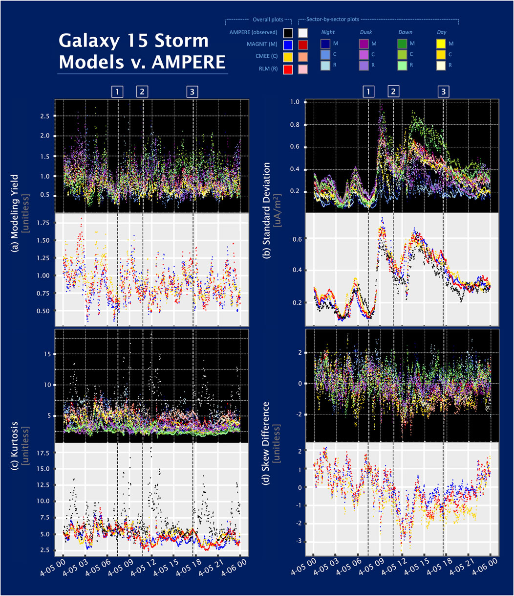
Figure 6. The performance of various model configurations grouped by MLTs across the storm are shown for (A) the precision metric YI (modeling yield), (B) the general quantity $\sigma$ (standard deviation), (C) the extreme metric $\kappa$ (kurtosis), and (D) the extremes metric $\gamma$ difference (skew difference). Precision metrics (A,B) are discussed in Sections 3.4.1, 3.4.2, and extremes metrics (C,D) are discussed in Sections 3.5.1, 3.5.2. The standard error on each metric is given in Table 3 and is not plotted on their respective graphs because of its small size, which was not clearly visible.

Figure 7

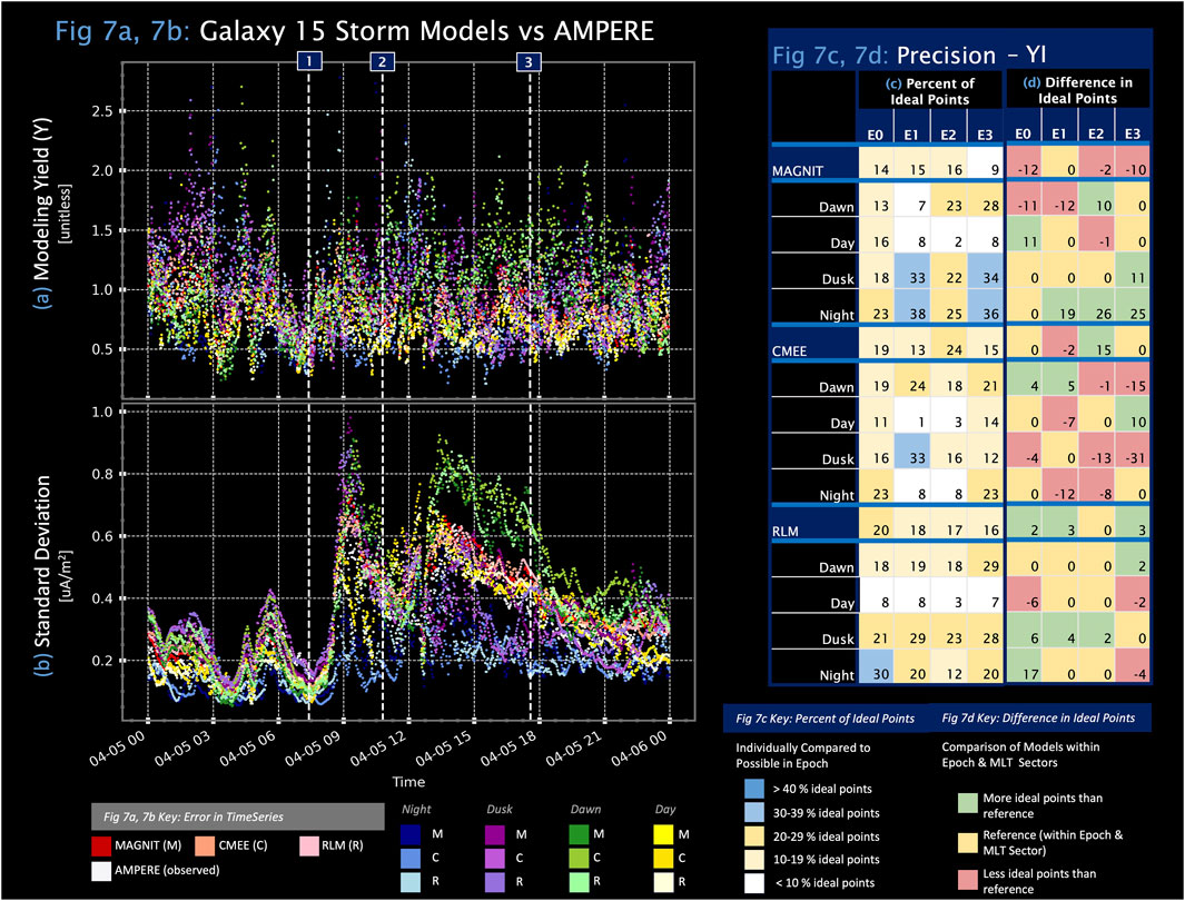
Figure 7. (A,B) describe the modeling yield (YI) and standard deviation $(\sigma )$ throughout the storm. Explanations of (C) and (D) type tables are covered in Sections 3.3. Additional interpretation of precision is provided in Sections 3.4.

3.4.1 Modeling yield

As Figure 6A and Figure 7A show, throughout the storm, all three models and their MLT groupings have generally good modeling yields. The modeling yield is calculated using just four numbers, the maximum and minimum of both the model and observed data, and thus suggests that the models can replicate the extent of the spread of the observed data. The modeling yield oscillates around 1, the ideal value, but a slightly denser population of YI points is less than the ideal value and has a smaller spread than AMPERE data. However, when models have a larger spread than the AMPERE data, the magnitude of the ratio between the model and observed spreads is larger. The three models have a larger spread in values during the storm activity, driven by a similar pattern observed in the dawn and dusk MLT sectors. Unlike dawn and dusk, the night and day sectors have a smaller spread than observed AMPERE data during the storm main phase. In this study, the data population distributions were calculated by grouping MLT sectors but could also be divided by latitudinal ranges. Although we focus on the global and holistic appraisal of conductance models in this paper, we expect improvement in YI values if future studies limit the latitudes to regions of consistent current structures.

Figures 7C, D provide numerical information on the precision performance for each model/MLT sector combination against AMPERE and against one another. The percent of ideal points in each epoch varies for model configuration throughout the storm. Overall, CMEE and RIM have an average of 17.75% and MAGNIT has an average of 13.5% of ideal points throughout the storm, as opposed to MLT sector investigations, where the three models are ranked in order by MAGNIT, RLM, and CMEE (MAGNIT/CMEE/RLM dawn: 17.75/20.5/21%, dusk: 26.75/19.25/25.25%, and night: 30/15.5/20.5%). The precision in the day sector is the worst across all three models during the main and recovery phases of the storm, averaging less than 8.5%. The number of ideal points improves during recovery to levels greater than those observed before the storm, especially in the dawn sector. Compared to the overall polar region precision performance, the MLT sector-by-sector has a larger divergence between the models.

3.4.2 Standard deviation

The standard deviation is frequently used in model performance assessment, and we use it here as well. Figure 6B and Figure 7B show the standard deviation of the various datasets. The spread in all values (including observed AMPERE data) increases significantly following extreme changes in $B_z$ and $B_y$ ($\sim$10:30 and $\sim$12:30 UT; Figure 1). The results observed in the modeling yield are confirmed in the standard deviation, which not only describes the extent of the distribution but also the shape. The standard deviations of the three models in the overall polar region are smaller than those in AMPERE pre-storm and larger than those in AMPERE during this active storm interval. Compared to the overall AMPERE dataset, the standard deviations of the night sector for all three models are small. In Epoch 2, dawn and dusk sectors have comparable FAC value distributions. Following the sudden IMF change at $\sim$10:30 UT, where all models and AMPERE have small spreads describing well-predicted peaks in FAC values, the day sector of the model best follows the standard deviation of AMPERE. In Epoch 3, the dawn sector data points have a larger spread in values, while the dusk and night sectors have a smaller distribution than those in AMPERE. As the storm activity decreases and the environment recovers, the spread in FAC values converges between the models and AMPERE. Within each MLT sector, the three models intertwine in performance over the storm.

3.5 Extremes: kurtosis, skew, and model-observed differences

In the subsection above, we provided information on model performance in replicating the mean of the observed data, and now offer understanding of the population away from the mean. Kurtosis describes the tailedness of the data distribution (how much of a tail exists in the data distribution), while skew characterizes the shift in the data distribution toward the tails. A normal distribution has a kurtosis value of 3 and a skew value of 0. Larger kurtosis values indicate that the population is leptokurtic and has a sharper peak, while smaller kurtosis values are for platykurtic populations with a broader sloped peak. In a positive skew, the population is shifted toward the left, and the mean is larger than the median and mode of the dataset. On the other hand, in a negative skew, the population is shifted rightward, and the most commonly occurring data point is larger than the median and mean. Similar to other metric categories, the performance of all three model configurations is comparable to observed AMPERE data. MAGNIT most closely resembles AMPERE in skew, while there is no clear lead in the performance of kurtosis. Across the various models and AMPERE FAC data, the night sector has a kurtosis value of $\sim 4$, suggesting a potential future investigation into alternatives over the use of a normalized distribution for auroral precipitation.

3.5.1 Kurtosis

Figure 8 follows the same structure as Figure 5A and Figure 7 and describes the performance of the three model configurations in terms of skew and kurtosis. Figure 6C, Figure 8B, and Table 2 show that the kurtosis values for MAGNIT, CMEE, and RLM have an average baseline of $\sim 4.8$, similar to AMPERE. In each MLT grouping, the models have lower average kurtosis values than over the entire auroral region: in order of MAGNIT, CMEE, and RLM—dawn 3.2/2.9/3.1, day 3.7/3.6/3.7, dusk 2.8/2.6/2.7, and night 4.2/3.7/4.3. The day and night MLT sectors have higher kurtosis values than dawn and dusk, more closely matching overall polar region values and following the shape of kurtosis increases and decreases in AMPERE better. However, the kurtosis values of the models in the night sector frequently jump suddenly to extremely large values $\sim 8$, largely independent of noticeable features in the AMPERE data and storm. Because kurtosis takes the difference between the model and observed values to the fourth power, outliers become susceptible to extreme values. Overall, however, the kurtosis differences are not extreme and are between 0 and $-2$, with the exceptions described above.

Figure 8

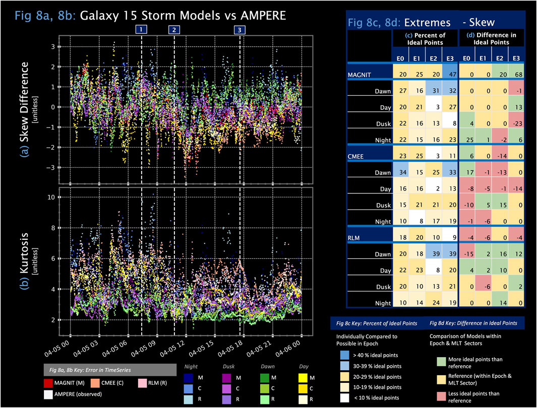
Figure 8. (A,B) Skew difference $({\gamma }_{\text{diff}})$ and kurtosis $(\kappa )$ throughout the storm. Explanations of (C) and (D) type tables are covered in Section 3.3. Additional interpretation of extremes is provided in Sections 3.5.

3.5.2 Skew differences

The skew in AMPERE varies throughout the storm, as shown in Figure 6D and Figure 8A. Before the storm, the dataset tends to skew negatively so that the mode is more often larger than the median and mean. During the storm activity, the opposite is true, from the first major change in $B_z$ in Epoch 1. Once recovery begins ($\sim$12:30 UT), the skews of the models remain nearly constant until the beginning of Epoch 3, where MAGNIT returns to a pre-storm positive skew, RLM has little to no skew, and CMEE continues to exhibit a negative skew. The skew observed in MAGNIT most closely follows the skew pattern of AMPERE. The behavior of the MLT sector is diverse: while the dusk and night sectors skew positively throughout the storm, dawn skews negatively, and day skews negatively starting in Epoch 1. An exception occurs at $\sim$12:30 UT, where $B_z$ changes significantly for the second time, and MLT sectors suddenly skew negatively. In any case, positive and negative skewness have similar magnitudes, with the maximum and minimum differences ranging between −2 and 2.

In general, compared to the modeling yield in precision and the mean bias error, the three models have more ideal points in skew difference during and after storm activity, as shown in Figures 8C, D. The three model overall configurations during epochs 0 and 1 have comparable performance, with $\sim$ 22% of points meeting the ideal point requirement, and differences are within 5% of one another. During epochs 2 and 3, the number of ideal points in MAGNIT increases while decreasing to less than half of pre-storm values for RLM and CMEE. This change is not reflected as significantly in the day, dusk, and night sectors of the three model configurations, where the performance in all three models is comparable to each other. The dawn sector (particularly in RLM) best reflects the skew observed in AMPERE, with 30%–40% ideal points.

4 Discussion

Generally, the performance of MAGNIT exceeds that of RLM and CMEE, but there are intricacies in model performance grouped by MLT sectors and through storm phases. In some metrics, CMEE shows better performance metrics on the global scale, but this pattern is not reflected in MLT divisions. Instead, MAGNIT’s performance surpasses that of CMEE and RLM in the MLT sectors. This result is summarized in the conclusion. There are several surprising outcomes from the metric analysis. In particular, they include the following points:

1. The performance of RLM and MAGNIT is more similar than that of the RLM and CMEE.

2. The night MLT sector consistently exhibits the best performance across all storm phases, conductance specifications, and most metrics.

In many of the metrics, the performance of MAGNIT and RLM was more similar than that of MAGNIT and CMEE or RLM and CMEE. This is particularly interesting since the RLM and CMEE are designed from similar empirical formats, albeit trained with different datasets. This trend may be a result of several factors. For example, the difference in events used to train RLM and CMEE implies that CMEE is a more statistical model because it is trained on more data and will adopt the characteristics of sparse extreme events. This analysis was conducted on a singular storm event, and model performances over other types of geospace conditions are unexplored. The Galaxy 15 event, a highly active event producing high levels of precipitation, has implications on day–night conductance that are unique in this validation study. As with any validation effort, more and different types of events help clarify use cases. Because MAGNIT can be run with different auroral precipitation sources, specific characteristics of MLT sectors can be associated with various auroral precipitation sources, helping us understand the similarities and differences between the three models. Unlike CMEE and RLM, MAGNIT can be improved by adding or modifying the physics in the code. This emphasizes the benefit of semi-physical over empirical models in modeling frameworks that need to accommodate a variety of use cases and quantities.

A common theme across many metric categories was the “better” performance of the night sector when data was investigated at different magnetic local time groupings. This theme can be explained in part by recognizing that spatial and temporal regions of high-magnitude conductance appear to exhibit lower errors throughout the study. The Galaxy 15 storm occurring near the equinox was a highly active event, initially producing a strong day-side compression and generating high activity on the night-side as the storm progressed. During sudden commencement, when day-side conductance is high, the error in the day-side by the models is small (Figures 4B, 5). This pattern is better represented on the night-side, where conductance remains high throughout storm activity because of elevated particle precipitation levels. This can be observed in the respective errors in the models, including in metrics on accuracy (Section 3.1), bias (Sections 3.3, 3.3.2), and precision (Section 3.4.2). The better performance of the night sector is somewhat expected—Mukhopadhyay et al. (2022b) and Mukhopadhyay (2021) used MAGNIT to study auroral precipitation contributions to the Galaxy 15 event and found that the largest contributor was the diffuse electron and ion precipitation sources, which favorably map toward the night-side. The electron and ion diffuse sources are dependent on MHD pressure, which peaks at night and slightly at dawn and dusk.

Another hypothesis on the comparably superior performance of the night sector is the inherent crescent shape of the FAC patterns, which is thinner in latitude spread at the edge MLT values. The bulk of FACs flows up and down into the ionosphere at dawn and dusk; hence, the night and day sectors contain some of these edge MLT values. In the night sector, the models can accurately replicate FACs at the latitude and longitude locations. Dawn and dusk FAC values were more likely to miss the measured value because the FACs produced by the models were wider in latitude. Wider FAC coverage allows for more space where small-scale features are shifted and reflect poorly on a one-to-one spatial comparison, leading to the “worst” performance across metrics and during storm activity. The day sector also lacks in performance compared to the night sector, contrary to what would be expected from the edge-thinning FAC region hypothesis. All three models use AMIE (RLM and CMEE utilize AMIE as a primary derivative, while MAGNIT uses its results as a supplement), which has been shown to underestimate electron flux and has a more accurate prediction in the 18:00–03:00 MLT partial dusk and full night-side sectors, where solar conductance is not as significant (Kihn and Ridley, 2005). Although the day sector generally underestimates the FAC magnitude, the modeling yield suggests that the maximum and minimum FACs are captured reasonably accurately by the models.

The metrics in this study agree well with previous efforts, including those obtained by Mukhopadhyay et al. (2022b) and Anderson et al. (2017). In extending the SWPC Geospace Environment Modeling (GEM) challenge to access the relative performance of predicting FACs, Anderson et al. (2017) compared the radial current of AMPERE and several models, including the SWMF (with RLM), quantifying the correlation coefficient. The SWMF R-values obtained by Anderson et al. (2017) are larger than those calculated in this study, possibly because of the comparison method. While this validation study uses a direct location and exact time comparison, Anderson et al. (2017) smoothed FAC values, meaning that our metrics could likely be improved by increasing the grid resolution of the model runs. An important limitation to note in validation studies, including this study, is the use of observations as a “ground truth.” The differences in spatial and temporal resolution between observations and models can introduce significant noise that can potentially mean that in some instances, modeling results can be better than observations and their derived estimates. The small standard deviation of the models pre-storm and during the night sectors (Section 3.4.2) of the storm provides such illustrations. On the night-side, in particular, the low R-value can also be attributed, for example, to a combination of low (near-0) FAC values and a small spread (low YI). Studying the effects of models and observation resolution is key to validating any model performance in the future. Despite the interesting performance of the three models in replicating the small-scale features of the FACs, the three SWMF IE configurations align well with large-scale features (for example, integrated FACs [Mukhopadhyay et al., 2022b]). They clearly and appropriately respond to storm-driving conditions. The most desirable SWMF IE configuration to run for different use cases is summarized in the conclusion.

In addition to comparing against AMPERE by latitudes, adding transitional MLT sectors (i.e., a dawn–day blend in between dawn and day) may help highlight MLT-specific characteristics. It may also provide insight into the mirroring effect found between the overestimation and underestimation of dusk and dawn or day. Since we demonstrated the advantages of investigating the data distribution in more detail in this study, we recommend that future model validation and verification efforts take advantage of diversifying statistics to help explain and investigate performance.

5 Conclusion

This study explored the performance of SWMF-RLM, SWMF-CMEE, and SWMF-MAGNIT in predicting FACs for the Galaxy 15 storm event (5 April 2010, 00:00–6 April, 00:00). The comparison base-lined model performance with AMPERE observationally derived values in a validation effort and was conducted by investigating a variety of statistical metrics including accuracy, bias, precision, association, and extremes.

FACs were not used as a comparator to train the model configurations. Although the integrated FACs in the ionosphere are demonstrated to be in good agreement with data obtained by the models (Mukhopadhyay et al., 2022b), the FAC pattern is not a direct replication of AMPERE data. As expected, model performance decreases during the storm main phase and returns to near pre-storm performance during event recovery. Sudden increases in error are attributed to violent activity in the storm and are reflected across metrics of different categories. While examining the correlation provided little insight into model performance, exploring bias, precision, and extreme characteristics of the model replications suggested paths for the investigation and development of future model improvements and inquiries.

In general, MAGNIT can be considered to have marginally better performance than CMEE and RLM. SWMF-MAGNIT has the lowest RMSE, is the least underestimating, and has both modeling yield and skew closest to the observed data. In the global polar region, however, CMEE has comparable or better performance: it has more ideal points in bias (ME) and precision. When breaking down bias and precision data by MLT sector, MAGNIT ranks better than CMEE. The advantage of MAGNIT is clearer in sector-by-sector investigations as MAGNIT MLT sectors have the smallest error compared to CMEE and RLM MLT sectors. The night sector has the lowest pure FAC value error throughout the storm, the least bias, and the most similar spread (to AMPERE), albeit a poor correlation. For the most part, this matches well with the pattern for a highly active storm, where areas with higher conductance correspond to smaller respective errors and the night sector, particularly in MAGNIT, with improved precipitation calculations exhibiting better performance. Day and dawn sectors are often the least reliable, and dawn and dusk performance varies the most. For example, dawn and dusk begin as the biggest contributors to the lack of accuracy, but as the storm continues, they shift to dawn and day. The differing performance in the various MLT sectors can be attributed to a variety of reasons, including the shape and mapping of the FACs, the involvement of various auroral precipitation sources, and the inclusion of auroral conductance from AMIE; furthermore, it suggests that additional physics in each MLT sector should be investigated and added to provide a thorough representation of the system. The poor performance of the non-night sectors, particularly in the spatial and temporal regions of low conductance, highlights the importance of the well-known complication in the coupling of the ionosphere and other regions. The metrics of all three model configurations are in agreement with previous validation work.

While additional analysis on different events can provide more fidelity to model validation and verification, this paper has demonstrated that exploring a number of performance metrics from different categories provides richer insights into space weather modeling.

Data availability statement

The datasets presented in this study can be found in online repositories. The names of the repository/repositories and accession number(s) can be found at: https://deepblue.lib.umich.edu/data/concern/data_sets/8g84mm73z [Deep Blue Data—Title: Data Pertaining to Initial Simulations Using the MAGNetosphere–Ionosphere–Thermosphere (MAGNIT) Auroral Precipitation Model].

Author contributions

EH: conceptualization, formal analysis, investigation, methodology, resources, validation, visualization, writing–original draft, and writing–review and editing. AM: conceptualization, data curation, resources, visualization, and writing–review and editing. ML: conceptualization, funding acquisition, investigation, resources, supervision, and writing–review and editing. TK: resources and writing–review and editing. BA: data curation, resources, and writing–review and editing. SV: data curation, resources, and writing–review and editing. RB: data curation, resources, and writing–review and editing.

Funding

The author(s) declare that financial support was received for the research, authorship, and/or publication of this article. This work was supported by the NSF Comprehensive Hazard Analysis for Resilience to Geomagnetic Extreme Disturbances (CHARGED), grant number 1663770, held by PI and ML.

Acknowledgments

The authors thank the AMPERE Science team for providing access to the Iridium-derived data products and the University of Michigan Magnetosphere, Ionosphere, Thermosphere s and Applied Science (MITHRAS) Group for sharing their expertise and advice in the writing of this paper and statistical analysis conducted as part of this study.

Conflict of interest

The authors declare that the research was conducted in the absence of any commercial or financial relationships that could be construed as a potential conflict of interest.

Publisher’s note

All claims expressed in this article are solely those of the authors and do not necessarily represent those of their affiliated organizations, or those of the publisher, the editors, and the reviewers. Any product that may be evaluated in this article, or claim that may be made by its manufacturer, is not guaranteed or endorsed by the publisher.

Footnotes

¹By directly, we mean that the quantity is a direct output not derived from combinations of other direct outputs.

²For example, the Michigan Geospace model was originally selected for operational use based on dB/dt performance but is used in the present day for dB/dt and Kp forecasts.

³This paper reviews seven metrics listed in Table 1 and does not include four additional metrics completed in the validation effort: (in accuracy) symmetric mean absolute percentage error and median symmetric accuracy, (in bias) symmetric signed percentage bias, and (in skill) prediction efficiency. Detailed reasoning is given in Section 2.3 “Statistical methods.”

⁴https://clasp.engin.umich.edu/research/theory-computational-methods/space-weather-modeling-framework/

⁵https://github.com/MSTEM-QUDA/SWMF

⁶https://ampere.jhuapl.edu

References

Anderson, B., Angappan, R., Barik, A., Vines, S., Stanley, S., Bernasconi, P., et al. (2021). Iridium communications satellite constellation data for study of earth’s magnetic field. AGU Geochem. Geophys. Geosystems 22. doi:10.1029/2020GC009515

CrossRef Full Text | Google Scholar

Anderson, B., Korth, H., Welling, D., Merkin, V., Wiltberger, M., Raeder, J., et al. (2017). Comparison of predictive estimates of high-latitude electrodynamics with observations of global-scale Birkeland currents. Space weather. 15, 352–373. doi:10.1002/2016SW001529

CrossRef Full Text | Google Scholar

Anderson, B., Takahashi, K., Kamei, T., Waters, L., and Toth, B. (2002). Birkeland current system key parameters derived from Iridium observations: method and initial validation results. JGR Space Phys. 107. doi:10.1029/2001JA000080

CrossRef Full Text | Google Scholar

Anderson, B., Takahashi, K., and Toth, B. (2000). Sensing global Birkeland currents with iridium® engineering magnetometer data. Geophys. Res. Lett. 27, 4045–4048. doi:10.1029/2000GL000094

CrossRef Full Text | Google Scholar

Boris, J. (1970). A physically motivated solution of the alfven problem. Tech. rep. Springfield, VA: National Technical Information Service.

Google Scholar

Edwards, T., Weimer, D., Olsen, N., Luhr, H., Tobiska, W., and Anderson, B. (2019). A third generation field-aligned current model. JGR Space Phys. 125. doi:10.1029/2019JA027249

CrossRef Full Text | Google Scholar

Glocer, A., Rastätter, L., Kuznetsova, M., Pulkkinen, A., Singer, H., Balch, C., et al. (2016). Community-wide validation of geospace model local K-index predictions to support model transition to operations. JGR Space Phys. 14, 469–480. doi:10.1002/2016SW001387

CrossRef Full Text | Google Scholar

Gombosi, T., and Nagy, A. (1989). Time-dependent modeling of field-aligned current-generated ion transients in the polar wind. JGR Space Phys. 94, 359–369. doi:10.1029/JA094iA01p00359

CrossRef Full Text | Google Scholar

Haiducek, J., Welling, D., Ganushkina, N., Morley, S., and Ozturk, D. (2017). SWMF global magnetosphere simulations of january 2005: geomagnetic indices and cross-polar cap potential. AGU Space Weather 15, 1567–1587. doi:10.1002/2017SW001695

CrossRef Full Text | Google Scholar

He, M., Vogt, J., Luhr, H., Sorbalo, E., Blagau, A., Le, G., et al. (2012). A high-resolution model of field-aligned currents through empirical orthogonal functions analysis (MFACE). JGR Space Phys. 39. doi:10.1029/2012GL053168

CrossRef Full Text | Google Scholar

Iijima, T., and Potemra, T. (1976). Field-aligned currents in the dayside cusp observed by Triad. JGR Space Phys. 81, 5971–5979. doi:10.1029/JA081i034p05971

CrossRef Full Text | Google Scholar

Kamide, Y. (1982). The relationship between field-aligned currents and the auroral electrojets: a review. Space Sci. Rev. 31, 127–243. doi:10.1007/BF00215281

CrossRef Full Text | Google Scholar

Kihn, E., and Ridley, A. (2005). A statistical analysis of the assimilative mapping of ionospheric electrodynamics auroral specification. JGR Space Phys. 110. doi:10.1029/2003JA010371

CrossRef Full Text | Google Scholar

Knight, S. (1973). Parallel electric fields. Planet. Space Sci. 21, 741–750. doi:10.1016/0032-0633(73)90093-7

CrossRef Full Text | Google Scholar

Lane, C., Acebal, A., and Zheng, Y. (2014). Assessing predictive ability of three auroral precipitation models using DMSP energy flux. JGR Space Phys. 13, 61–71. doi:10.1002/2014SW001085

CrossRef Full Text | Google Scholar

Le, G., Slavin, J., and Strangeway, J. (2010). Space Technology 5 observations of the imbalance of regions 1 and 2 field-aligned currents and its implication to the cross-polar cap Pedersen currents. JGR Space Phys. 115. doi:10.1029/2009JA014979

CrossRef Full Text | Google Scholar

Liemohn, M. (2020). The case for improving the Robinson formulas. JGR Space Phys. 125. doi:10.1029/2020JA028332

CrossRef Full Text | Google Scholar

Liemohn, M., Ridley, A., Kozyra, J., Gallagher, D., Thomsen, M., Henderson, M., et al. (2006). Analyzing electric field morphology through data-model comparisons of the geospace environment modeling inner magnetosphere/storm assessment challenge events. JGR Space Phys. 111. doi:10.1029/2006JA011700

CrossRef Full Text | Google Scholar

Liemohn, M., Shane, A., Azari, A., Petersen, A., Swiger, B., and Mukhopadhyay, A. (2021). RMSE is not enough: guidelines to robust data-model comparisons for magnetospheric physics. J. Atmos. Solar-Terrestrial Phys. 218, 105624. doi:10.1016/j.jastp.2021.105624

CrossRef Full Text | Google Scholar

Loto’aniu, T., Singer, H., Rodriguez, J., Green, J., Denig, W., Biesecker, D., et al. (2015). Space weather conditions during the Galaxy 15 spacecraft anomaly. JGR Space Phys. 13, 484–502. doi:10.1002/2015SW001239

CrossRef Full Text | Google Scholar

Lysak, R. (1990). Electrodynamic coupling of the magnetosphere and ionosphere. Space Sci. Rev. 52, 33–87. doi:10.1007/bf00704239

CrossRef Full Text | Google Scholar

Mukhopadhyay, A. (2021). Sources of auroral precipitation: balance, impacts and drivers. Doctoral dissertation. Ann Arbor, Michigan: University of Michigan.

Google Scholar

Mukhopadhyay, A., Glocer, A., Welling, D., Garcia-Sage, K., Liemohn, M., Burleigh, M., et al. (2022a). “Global prediction of auroral electrodynamics-source balance and hemispheric asymmetries,” in AGU Fall Meeting, Chicago, IL, 12 - 16 December 2022.

Google Scholar

Mukhopadhyay, A., Welling, D., Liemohn, M., Ridley, A., Burleigh, M., Wu, C., et al. (2022b). Global driving of auroral precipitation: 1. Balance of sources. JGR Space Phys. 127, e2022JA030323. doi:10.1029/2022JA030323

CrossRef Full Text | Google Scholar

Mukhopadhyay, A., Welling, D., Liemohn, M., Ridley, A., Chakraborty, S., and Anderson, B. (2020). Conductance model for extreme events: impact of auroral conductance on space weather forecasts. Space weather. 18. doi:10.1029/2020SW002551

CrossRef Full Text | Google Scholar

Nishimura, Y., Lyons, L., Gabrielse, C., Sivadas, N., Donovan, E., Varney, R., et al. (2020). Extreme magnetosphere-ionosphere-thermosphere responses to the 5 April 2010 supersubstorm. JGR Space Phys. 125. doi:10.1029/2019JA027654

CrossRef Full Text | Google Scholar

Powell, K., Roe, P. L., Linde, T., Gombosi, T., and DeZeeuw, D. (1999). A solution-adaptive upwind scheme for ideal magnetohydrodynamics. J. Comput. Phys. 154, 284–309. doi:10.1006/jcph.1999.6299

CrossRef Full Text | Google Scholar

Pulkkinen, A., Rastatter, L., Kuznetsova, M., Singer, H., Balch, C., Weimer, D., et al. (2013). Community-wide validation of geospace model ground magnetic field perturbation predictions to support model transition to operations. Space weather. 11, 369–385. doi:10.1002/swe.20056

CrossRef Full Text | Google Scholar

Pulkkinen, T., Gombosi, T. I., Ridley, A. J., Toth, G., and Zou, S. (2021). The Space Weather Modeling Framework goes open access. EOS, 102. doi:10.1029/2021EO158300

CrossRef Full Text | Google Scholar

Raeder, J., Larson, D., Li, W., Kepko, E., and Fuller-Rowell, T. (2008). OpenGGCM simulations for the THEMIS mission. Space Sci. Rev. 27. doi:10.10207/s11214-008-9421-5

CrossRef Full Text | Google Scholar

Ridley, A., Gombosi, T., and DeZeeuw, D. (2004). Ionospheric control of the magnetosphere: conductance. Ann. Geophys 22, 567–584. doi:10.5194/angeo-22-567-2004

CrossRef Full Text | Google Scholar

Ritter, P., Luhr, H., and Rauberg, J. (2013). Determining field-aligned currents with the Swarm constellation mission. Earth, Planets Space 65, 1285–1294. doi:10.5047/eps.2013.09.006

CrossRef Full Text | Google Scholar

Saflekos, N., Sheehan, R., and Carovillano, R. (1982). Global nature of field-aligned currents and their relation to auroral phenomena. Rev. Geophys. 20, 709–734. doi:10.1029/RG020i003p00709

CrossRef Full Text | Google Scholar

Sergeev, V., Angelopoulos, V., Kubyshkina, M., Donovan, E., Zhou, X., Runov, A., et al. (2011). Substorm growth and expansion onset as observed with ideal ground-spacecraft THEMIS coverage. JGR Space Phys. 16. doi:10.1029/2010JA015689

CrossRef Full Text | Google Scholar

Toffoletto, F., Sazykin, S., Spiro, R., and Wolf, R. (2003). Inner magnetospheric modeling with the Rice convection model. Space Sci. Rev. 107, 175–196. doi:10.1023/A:1025532008047

CrossRef Full Text | Google Scholar

Toth, G., Sokolov, I., Gombosi, T., Chesney, D., Clauer, C., DeZeeuw, D., et al. (2005). Space Weather Modeling Framework: a new tool for the space science community. JGR Space Phys. 110. doi:10.1029/2005JA011126

CrossRef Full Text | Google Scholar

Tóth, G., van der Holst, B., Sokolov, I., DeZeeuw, D., Gombosi, T., Fang, F., et al. (2012). Adaptive numerical algorithms in space weather modeling. J. Comp. Phys. 231, 870–903. doi:10.1016/j.jcp.2011.02.006

CrossRef Full Text | Google Scholar

Watanabe, M., Iijima, T., Nakagawa, M., Potemra, T., Zanetti, L., Ohtani, S., et al. (1998). Field-aligned current systems in the magnetospheric ground state. JGR 103, 6853–6869. doi:10.1029/97JA03086

CrossRef Full Text | Google Scholar

Waters, C., Anderson, B., and Liou, K. (2001). Estimation of global field aligned currents using the iridium® System magnetometer data. Geophys. Res. Lett. 28, 2165–2168. doi:10.1029/2000GL012725

CrossRef Full Text | Google Scholar

Waters, C. L., Anderson, B., Green, D., Korth, H., Barnes, R., and Banhamaki, H. (2020). Ionospheric multi-spacecraft analysis tools: science data products for AMPERE. ISSI Sci. Rep. Ser. 17, 141–165. doi:10.1007/978-3-030-26732-2_7

CrossRef Full Text | Google Scholar

Weimer, D. (2001). Maps of ionospheric field-aligned currents as a function of the interplanetary magnetic field derived from Dynamics Explorer 2 data. JGR Space Phys. 106, 12889–12902. doi:10.1029/2000JA000295

CrossRef Full Text | Google Scholar

Zeeuw, D. D., Sazykin, S., Wolf, R., Gombosi, T., Ridley, A., and Toth, G. (2004). Coupling of a global MHD code and an inner magnetospheric model: initial results. JGR Space Phys. 109. doi:10.1029/2003JA010366

CrossRef Full Text | Google Scholar

Zhang, B., Sorathia, K., Lyon, J., Merkin, V., Garretson, J., and Wiltberger, M. (2000). GAMERA: a three-dimensional finite-volume MHD solver for non-orthogonal curvilinear geometries. Astrophys. J. 244, 20. doi:10.3847/1538-4365/ab3a4c

CrossRef Full Text | Google Scholar