 Hassanali Akbari
 Douglas Rowland
 Austin Coleman3
 Jeffrey Thayer
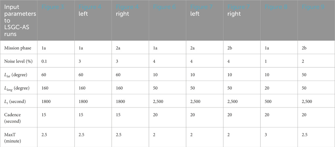

94% of researchers rate our articles as excellent or good
Learn more about the work of our research integrity team to safeguard the quality of each article we publish.
Find out more
METHODS article
Front. Astron. Space Sci., 29 February 2024
Sec. Space Physics
Volume 11 - 2024 | https://doi.org/10.3389/fspas.2024.1231840
This article is part of the Research TopicPast, Present and Future Of Multispacecraft Measurements For Space PhysicsView all 10 articles
The upcoming Geospace Dynamics Constellation (GDC) mission aims to investigate dynamic processes active in Earth’s upper atmosphere and their local, regional, and global characteristics. Achieving this goal will involve resolving and distinguishing spatial and temporal variability of ionospheric and thermospheric (IT) structures in a quantitative manner. This, in turn, calls for the development of sophisticated algorithms that are optimal in combining information from multiple in-situ platforms. This manuscript introduces an implementation of the least-squares gradient calculation approach previously developed by J. De Keyser with the focus of its application to the GDC mission. This approach robustly calculates spatial and temporal gradients of IT parameters from in-situ measurements from multiple spacecraft that form a flexible constellation. The previous work by De Keyser, originally developed for analysis of Cluster data, focused on 3-D Cartesian geometry, while the current work extends the approach to spherical geometry suitable for missions in Low Earth Orbit (LEO). The algorithm automatically provides error bars for the estimated gradients as well as the scales over which the gradients are expected to be constant. We evaluate the performance of the software on outputs of high-resolution global ionospheric/thermospheric simulations. It is shown that the software will be a powerful tool to explore GDC’s ability to answer science questions that require gradient calculations. The code can also be employed in support of Observing System Simulation Experiments to evaluate suitability of various constellation geometries and assess the impact of measurement sensitivities on addressing GDC’s science objectives.
Determining and disentangling the spatial and temporal variability of a field from sparse in-situ measurements is a long-standing problem in space physics. Addressing this problem, along with providing broader coverage in measurements, is commonly raised as a major justification for designing and launching multi-platform satellite missions (e.g., Escoubet et al., 2001; Burch et al., 2016). The Geospace Dynamics Constellation (GDC) mission, that is currently in the formulation phase, is one of the latest of such missions. GDC’s goal is to significantly increase our understanding of how the coupled ionosphere-thermosphere (IT) system reacts to external energy input from the Sun and the magnetosphere. Specifically, it will aim to address the following overarching science goals: 1) Understand how the high latitude ionosphere-thermosphere system responds to variable solar wind/magnetosphere forcing; and 2) Understand how internal processes in the global ionosphere-thermosphere system redistribute mass, momentum, and energy. Successfully addressing these objectives is challenging as the IT system is known to vary locally and globally, with scale-sizes ranging from sub-kilometer to thousands of kilometers and on timescales that range from seconds or minutes to hours or days.
Completely characterizing the dynamics of the IT system and determining the physical processes underlying its variability would ideally require a very dense (in altitude, longitude, and latitude) sampling of various plasma and neutral parameters over a wide range of spatial and temporal scales. As a practical matter, the number of spacecraft in such a constellation that can provide accurate comprehensive measurements is finite—for example, GDC will fly six spacecraft. This immediately introduces important challenges. On the one hand, relatively fine spatial and temporal resolutions, when compared to the physical scales, are required to properly capture the behavior of the system locally; and on the other hand, the global nature of the GDC mission would require a broad coverage of observing platforms in local time and longitude. Satisfying both conditions with a limited number of in-situ platforms can only be possible via a flexible constellation that evolves to observe the full range of relevant scales. A flexible satellite architecture, in turn, requires sophisticated algorithms that are themselves flexible and optimal in combining observations from individual points.
In this paper, we introduce a software package ‘LSGC-AS-LEO 1.0’, which is an implementation of the least-squares gradient calculation approach developed by De Keyser et al. (2007) and De Keyser (2008) with the focus on its application for the GDC mission. The gradients characterize variations of the field in space and time, helping to disentangle the spatial and temporal ambiguity in measurements in an inherently quantitative manner. In the following section, we briefly describe GDC’s expected constellation architecture and its evolution during different phases of the mission. In Section 3, we present a brief overview of the gradient calculation technique. In Section 4, we evaluate the performance of the technique on simulated GDC measurements of the IT parameters, and discuss its significance for the GDC mission. Section 5 includes the summary, conclusions, and a description of the future steps.
GDC’s constellation consists of six spacecraft in a circular orbit at the altitude of 350–400 km with an inclination of about 81–82°. At a given time, the spacecraft will sample plasma and neutral parameters on a relatively thin spherical shell, the altitude of which will slowly vary between 350 and 400 km due to orbital drag and subsequent reboosts via onboard propulsion. The satellites will be deployed via a single launch vehicle with small inclination differences. Over time, differential precession will lead to separation of the six orbital planes in local time, leading to an ever-widening instantaneous longitudinal coverage. Different phases of the mission can then be defined that are appropriate for the investigation of the IT processes over local (referred to as phase 1, with scale-lengths
Figure 1 shows the expected evolution of the satellite configuration during days 92 (top), 190 (middle), and 764 (bottom) from the start of the science phase of the mission. These correspond to the beginning of phase 1, end of phase 1, and sometime in the late regional/early global phase of the mission, respectively. Shown in each panel are instantaneous positions of all six spacecraft (shown as colored circles) for a scenario where the constellation is in the northern hemisphere and traveling northward. Thin vertical and horizontal lines show 5-degree increments in longitude and latitude. Dashed lines in colors matching each circle show the near future trajectory of that GDC spacecraft, demonstrating near-latitudinal direction around the equator, and predominantly longitudinal direction above ∼75° geographic latitude. Figure 1 clearly demonstrates the dynamic nature of the constellation in space and time and the complexities that one may face when attempting to determine spatio-temporal variability of the ionosphere and thermosphere from GDC measurements. For example, the hexagonal shape of the constellation seen in Panel A1 near the equator may be suitable to simultaneously determine local variability in latitude, longitude, and time; while at higher latitudes (see Panel A6), where the trajectories of the individual spacecraft cross, little information can be obtained in latitude due to lack of broad latitudinal sampling. In this case, the form of the constellation which briefly approximates a ‘pearls on a string’ configuration would be better suited for investigating variability in longitude and time.
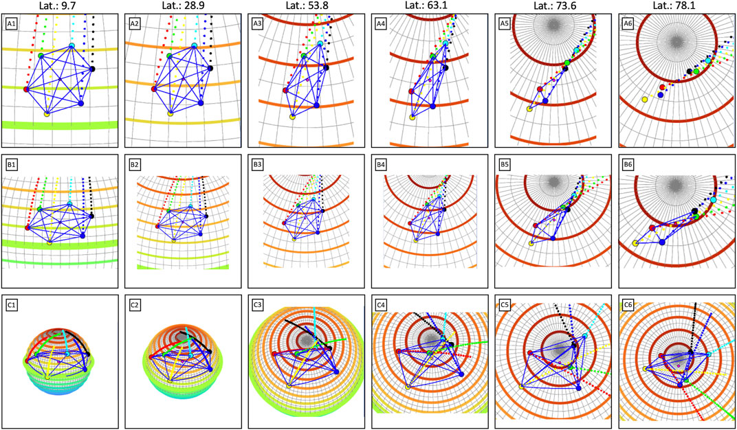
FIGURE 1. The expected evolution of the satellite configuration for days 92 (top), 190 (middle), and 764 (bottom) from the start of the science phase of the mission. Instantaneous positions of all six spacecraft (shown as colored circles) and the near future trajectory of that GDC spacecraft (shown as dashed lines in matching colors) are shown. Thin vertical and horizontal lines show 5-degree increments in longitude and latitude. The GDC ephemeris used here are from the ‘Revision C’ version, released in May 2022. The latest ephemeris is publicly available at https://ccmc.gsfc.nasa.gov/mission-planning/GDC/.
The variability in constellation architecture along with the need to monitor its ability to estimate gradients in both latitude and longitude at a given time motivated the creation of a quantity called the ‘quality’ (or ‘Q’) value and the associated ‘Q-vector’. The Q-value can be defined as
Figure 2 shows the trajectories of GDC spacecraft as a function of latitude and longitude (top panels) for three orbits corresponding to the beginnings of phases 1a (left), 2a (middle), and 3a (right). For each case, the magnitude and angle of the Q-vector is shown in the bottom panels as the constellation evolves in time. The drop in the magnitude of the Q-value is evident at high latitudes, consistent with the anisotropic constellation shape shown in Figure 1. As will be shown in Section 4, the ability of LSGC-AS-LEO 1.0 to fully determine both longitudinal and latitudinal variability in the IT system using GDC measurements may reduce for smaller Q-values below a threshold. Q-vector can, thus, be used as an empirical measure to optimize constellation design and provide an indication of where robust gradient calculations may be achievable.
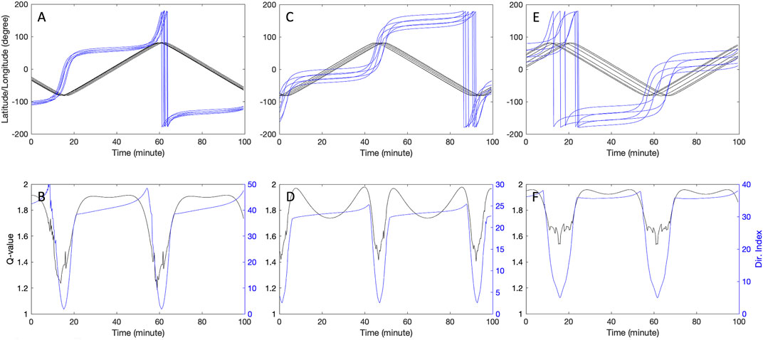
FIGURE 2. (A,C,E) GDC constellation latitudes (black) and longitudes (blue) for three orbits on the first days of phases 1a, 2a, and 3a, respectively. (B,D,E) parameters of the Q-vector for the orbits shown above.
Figure 1 and Figure 2 demonstrate the variability of GDC’s constellation geometry as a function of latitude and mission phase. As a result of this variability, any approach that would aim to utilize multi-point measurements from GDC to characterize the dynamics of the IT system would ideally need to be general and flexible, without many assumptions on the sampling scheme, and at the same time ensure the optimum utilization of data from all satellites. Further, a successful approach would need to take into account spatial and temporal scales over which ionospheric and thermospheric structures evolve relative to the size of the constellation, and provide measures of reliability for its calculations. The least-squares gradient calculation with adaptive scaling (LSGC-AS method, De Keyser et al., 2007; De Keyser, 2008) is such an approach and is briefly described in the next section.
Optimally combining information from multi-point measurements to quantitatively determine the local dynamics of a measured field often proves to be challenging. This topic has been the subject of many previous works that have let to the development of different algorithms and tools (e.g., Chanteur, 1998; Harvey, 1998; Paschmann and Daly, 1998; Robert et al., 1998; Amm and Viljanen, 1999; Darrouzet et al., 2006; Denton et al., 2020; Dunlop and Lühr, 2020; Fiori, 2020; Torbert et al., 2020; Bard and Dorelli, 2021; Denton et al., 2022; Zhu et al., 2022). Mathematically, the problem can be translated to one involving calculation of gradients—once the gradients of a field are known with respect to space and time its local dynamics can be better understood. Precise calculations of gradients, however, are generally difficult due to a number of reasons, the most important of which are the presence of noise in data and under-sampled variations of the measured field in between the spacecraft. On the one hand, for estimated gradients to be accurate the spacecraft should form a close constellation to fully resolve variations of the sampled field; and on the other hand, for the estimated values to be meaningful the difference between sampled values should be large compared to the measurement noise—a condition which may require a larger separation between the spacecraft. It is balancing between the two constraints that necessitates the use of sophisticated algorithms for computing gradients. In addition, the spatial scales of variation in the sampled field may vary depending on the process being studied, or the location of the measurements, which introduces further complexity and a need for the algorithm to assess its own performance. Given the complexity of the task of calculating gradients, a significant amount of effort has gone towards developing appropriate algorithms and tools. Much of these works have been performed in support of the European Space Agency’s (ESA) three-satellite Swarm mission (Friis-Christensen et al., 2008). For example, Ritter and Lühr (2006) and Ritter et al. (2013) were among the first to address current estimation in the context of a multi-satellite LEO mission. Vogt et al. (2009) and Vogt et al. (2013) provided tools and an error analysis framework for planar spacecraft configurations with special consideration of physical constraints to estimate out-of-plane contributions. Shen et al. (2012a) and Shen et al. (2012b) developed magnetic gradient estimation techniques with particular relevance to measurements in an environment dominated by field-aligned currents. Blagau and Vogt (2019) and Blagau and Vogt (2023) implemented relevant techniques in a publicly available software package based on Python. Of the mentioned works, those described by Shen et al. (2012b) and Vogt et al. (2020) stand out as general approaches to gradient calculations, both of which utilize some adaptation of the position tensor of the satellite configuration to compute spatial gradients in a least-squares sense. Very recently, in the past 2 years, a series of publications have emerged that introduce further methods to combine information from multiple in-situ platforms. These recent works include: Shen and Dunlop (2023), who introduced a geometrical method based on integral theorems to compute the linear gradients; Shen et al. (2021b), who developed a novel method to estimating both the linear and quadratic gradients using multiple spacecraft observation; Shen et al. (2021a) and Dunlop et al. (2021), who developed algorithms specifically for determining nonlinear magnetic gradients; and the book by Dunlop et al. (2021), that covers a number of multispacecraft techniques that were initially developed to analyze data from the Cluster mission (Escoubet et al., 2001). As mentioned before, here we implement the approach described by De Keyser et al. (2007) and De Keyser (2008), which is also a general gradient calculation tool, developed based on the concept of homogeneity scales in orthogonal directions, including in time. The method aims to ensure the utilization of the maximum amount of information available and allows to assess the meaningfulness of the result by providing error estimates. This approach is briefly described below. The description only includes high-level intuition behind the approach and is not meant as a substitute for the detailed mathematical description in De Keyser et al. (2007) and De Keyser (2008).
Imagine a scalar field f sampled at xi = [xi; yi; zi; ti], for i = 1⋯N, by an arbitrary number of satellites that form a flexible constellation. At a given time, f may be approximated in the vicinity of point x0 = [x0; y0; z0; t0] via its Taylor series expansion:
Much of the complexity of the weighted least-squares minimization approach mentioned above is condensed in obtaining proper weights, wi, for each equation based on the expected error associated with the corresponding measured sample. The choice of weights as inverse of the total error is to ensure that measurements with large errors do not contribute much to the solution of the over-determined system of equations. In the absence of systematic errors, the error δfi in estimating sample fi via fa(xi) may include three components. One is the ‘measurement error’ which is the inherent uncertainty associated with the instrument that provides fi; the second is the ‘approximation error’ (or the ‘curvature error’) which exists due to ignoring the nonlinear terms of the Taylor expansion in fa(x); and the third is the error due to the potential presence of unresolved small-scale fluctuations in the field. As described by De Keyser et al. (2007), the small-scale fluctuation error can be incorporated in a statistical sense, the measurement error can be modeled via a zero-mean random noise with a standard deviation specific to each instrument, and the approximation error can be modeled as
The homogeneity scales are properties of the physical field and change in space and time. In general, their determination is not trivial. De Keyser (2008) has described an approach to automatically determine the homogeneity scales from the measurements. The approach could be best understood by noting that solving the weighted over-determined system is equivalent to minimizing χ2, where:
However, one should bear in mind that in the presence of measurement and curvature errors, minimizing χ2 may not be a suitable target. In reality, the computations should be performed such that the residue ri reflect the correct amount of expected error associated with the calculations at point xi. In other words, one would reasonably expect that
The process of identifying the homogeneity scales, and consequently solving the over-determined system of equations, then starts from a set of initial guesses for the homogeneity scales, followed by the calculation of the total expected error for each measurement point, assigning weights to each equation, computing the gradients, determining χ2, then updating the homogeneity scales based on the value of χ2. This cycle may be incorporated in an optimization scheme to allow χ2 → 1 after a number of iterations. Several optimization approaches are introduced in De Keyser (2008). We have currently implemented the ‘common rescaling’ approach, which will be further discussed in the context of Figure 5. Future work will involve implementing the other approaches developed by De Keyser (2008) and exploring additional ones.
Motivated by the upcoming GDC mission, and with the goal of evaluating the ability of the satellite constellation to resolve local dynamics of the IT system, we have implemented the approach in an open-source software LSGC-AS-LEO 1.0, presently written in MATLAB. Despite the immediate focus of the software on GDC, LSGC-AS-LEO 1.0 is implemented in a general form, utilizing many settings that can be adjusted by the user, and as such it maintains the ability to support other missions with minimal updates to few functions. Here, we present and discuss typical outputs of the software on synthetic and simulated fields relevant to the IT system. Evaluating the results using simple synthetic test cases allows to validate the implementation, examine the robustness of the underlying algorithms, and further provides the opportunity to clarify certain important concepts of the algorithm described in Section 3 and in De Keyser et al. (2007) and De Keyser (2008). Additional test cases using realistic global simulations of the IT system along with GDC’s proposed ephemeris data further allows showcasing the significance of the software for GDC’s future measurements. Because GDC’s measurements will occur in a narrow altitude region between 350 and 400 km, our implementation of the LSGC-AS algorithm is tailored to assume spherical coordinates, and to assume zero radial variation, i.e., all measurement points are sampled at the same altitude and all the gradient calculations are performed in the spherical coordinates. Extending this procedure to account for non-zero radial variations is straightforward.
For the first test case, imagine a synthetic thermospheric neutral temperature of the form
where θ, ϕ, and t are latitude, longitude, and time in units of degree, degree, and seconds, respectively. Tn is not meant to represent the actual neutral temperature in the thermosphere; instead it serves as a simple function with simultaneous variability in latitude, longitude, and time. Running the software with an appropriate label specifying the synthetic function results in the following actions: GDC’s predicted ephemeris data over a predefined period of time are imported and used to sample the synthetic Tn with an adjustable cadence; a predefined level of measurement noise is then introduced to the sampled values; datapoints [xi, fi] from all or selected spacecraft gathered within a period of time centered at ti are then passed onto a routine in order to determine the gradients at point xi. The gradients are calculated at an arbitrary ‘evaluation point’, which by default is defined at the geometric center of the constellation. An optimization routine is used that adaptively modifies the homogeneity scales such that computations result in an appropriate outcome for χ2. Various settings that define the details of the computations are specified prior to running the routine. These include the initial guesses for homogeneity scales, fc, the measurement noise level, available satellites, the phase and time of the GDC mission, the evaluation point, optimization method, measurement cadence, integration time, whether calculations are performed on f or log(f), etc. The final result is an estimate of the value of Tn at the evaluation point, the longitudinal and latitudinal gradients of Tn at the evaluation point, the temporal rate of change of Tn at the evaluation point, and error bars for these quantities, as well as estimates for the homogeneity lengths.
Figure 3 shows the results of the gradient calculations for the synthetic function Tn sampled during the first 100 min of GDC’s phase 1a. The input parameters to LSGC-AS-LEO that have been used to produce this and the following plots are summarized in Table 1. In the top panel of Figure 3, Tn, as seen by six individual satellites, are shown with thin black lines. The size of the constellation in phase 1a is small compared to the scales over which Tn varies in space and time, and as a result the six spacecraft measure relatively similar values—i.e., the black lines nearly overlay each other—with the exceptions at the highest latitudes near times 14 and 60 min. Also shown in Panel A are the true (red) and the estimated (blue) values of Tn at the evaluation point, here defined as the center of the constellation. The calculated latitudinal, longitudinal, and temporal gradients along with their expected errors (i.e., their 3 − σ error bars) are shown in Panels B–D in blue. The calculated gradients closely follow the true gradients which are shown in red, with the exceptions at times ∼14 and 60 min where ∇latTn briefly deviates from the red curve and its error bars significantly increase. Noting the latitude and longitude of the evaluation point and the components of the Q-vector in Panels E and F, respectively, it becomes clear that the difficulty in determining ∇latTn (the latitudinal vector component of the gradient) around times ∼14 and 60 min is due to the shape of the constellation as the spacecraft approach the polar regions. As was shown in Panel A6 of Figure 1, at these times (primarily poleward of 75° geographic latitude in either hemisphere) the constellation spreads along longitude without much coverage in latitude, leading to poorly-constrained estimates for ∇latTn. This longitudinal elongation of the constellation is also reflected in Panel G which shows the condition number defined in De Keyser et al. (2007) as
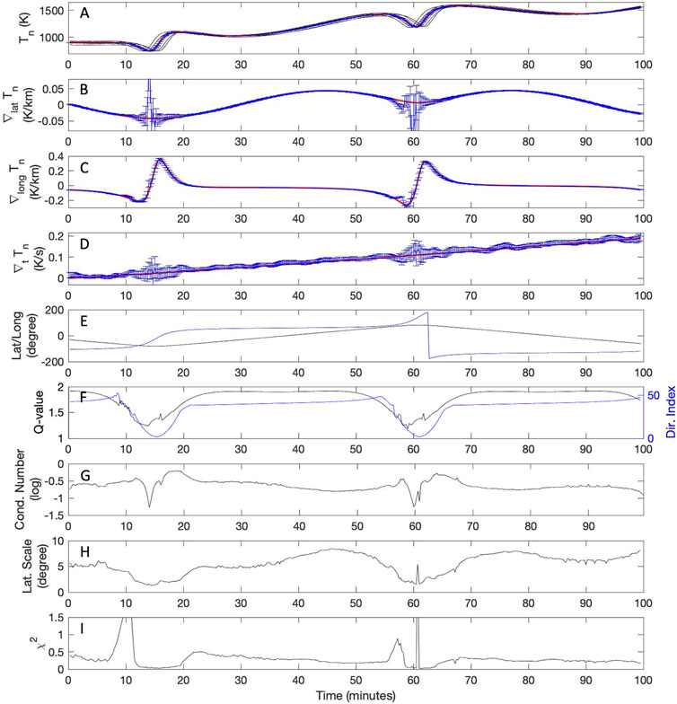
FIGURE 3. From top to bottom: (A) function values as observed by individual satellites (thin black lines), true (red), and reconstructed (blue) values of the function at the evaluation point, at the center of the constellation; (B) true (red) and estimated (blue) latitudinal gradients at the evaluation point; (C) true (red) and estimated (blue) longitudinal gradients at the evaluation point; (D) true (red) and the estimated (blue) temporal gradients at the evaluation point; (E) latitude (black) and longitude (blue) of the evaluation point; (F) components of the Q-vector; (G) condition number; (H) latitudinal homogeneity length Llat; (I) χ2. Synthetic function is sampled during the first 100 min of phase 1a, and is subjected to a small measurement noise of 0.1%. Other settings include: initial guesses for homogeneity length scales Llat: 60°, Llong: 160°, Lt: 1,800 s; maximum ‘time window’ over which to combine samples MaxT: 2.5 min; Measurement cadence: 15 s. The input parameters to LSGC-AS-LEO that have been used to produce various plots in this paper are summarized in Table 1.
It will be insightful to repeat the gradient calculation test described above with slight modifications. In the left panels of Figure 4 we show the results from a similar run in which the measurement error introduced to Tn is now significantly increased from 0.1% to 3% of fi. This is an important test as GDC will include various particle and field instruments with different levels of measurement accuracy for which the performance of the gradient calculation need to be tested. As can be seen in Panels A–D, an immediate consequence of the elevated noise level is larger errors for the calculated gradients, which are also reflected by the increased error bars. This is not surprising since gradient calculations are highly sensitive to the presence of background noise. Further, it is seen that, unlike in Figure 3B, the incorrect latitudinal gradients between 13–19 and 59–62 min are no longer properly covered by the error bars—this is perhaps due to inaccurate choices of initial homogeneity scales or fc. Nevertheless, the decreased condition number at these times can still serve as a cautionary flag regarding the accuracy of the results. In the right panels of Figure 4 we show the results from a similar run with yet another modification: the time axis now corresponds to the first 100 min of GDC’s phase 2b. In this phase the constellation size (i.e., the average distance between spacecraft) increases. The individual spacecraft now sample different values of Tn with differences that are greater than the 3% background noise level—see Panel J. Consequently, the accuracy of the estimated gradients increases and their error bars significantly drop in Panels K–M. This is due to the reduced noise amplification nature of the gradient operator over longer distances, and applies to cases where the measurement error dominates over the approximation error.
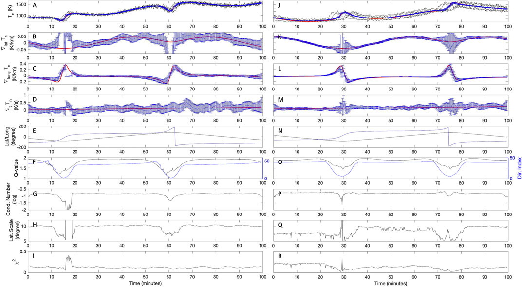
FIGURE 4. In the same format as that in Figure 3, but with increased added measurement noise level of 3%. The left and right panels correspond to the first 100 min of GDC’s phases 1a and 2a, respectively.
Before wrapping up the evaluation of the gradient calculation approach on the synthetic field Tn, it would be helpful to revisit the impact of the optimization and the adaptive scaling of the homogeneity lengths from a different prospective. Consider the results shown in Figure 4J–R at the single time t0 = 74.75 min. Here, the constellation approached the polar regions with the latitude of the evaluation point at 80.1°. At this time, about 120 samples [xi, fi], collected by all six spacecraft within 2.5 min from t0, have been used to calculate the gradients shown in panels K–M. According to Panel H, the optimization has decreased the homogeneity lengths by a common factor of about 7, from the initial scales of Llat = 60°, Llong = 160°, and Lt = 30 min. In Figure 5 we show the distribution of the residues |ri| for each datapoint xi as a function of the normalized distance |xi − x0|β. The absolute value of the residues are shown for the following two cases: the black datapoints correspond to the case where the least-squares minimization problem is solved without the optimization procedure (thus, only according to the initial homogeneity lengths); whereas the blue datapoints correspond to the case where the optimization has been turned on (thus allowing the homogeneity lengths to be rescaled). For the case of adaptive scaling turned off, the least-squares minimization approach is successful in solving the over-determined system of equations such that the residues are small and on the order of the measurement noise added to fi (shown by the horizontal black bar). Despite the reasonably small residues, however, we note that the gradients calculated using the initial homogeneity scales do not correctly represent the actual values—in other words, the calculated gradients are legitimate, yet inappropriate, solutions of the over-determined system. With adaptive scaling enabled, the homogeneity scales decrease, |xi − x0| increases, and as a result only a fraction of the datapoint that are closest to evaluation point are effectively used to calculate the gradients. The calculated gradients in latitude, longitude, and time are then modified by −96, 97, and −740%, respectively, compared to the previous case which brings them very close to the true gradients. At the same time, we observe that the distribution of |ri| as a function of the normalized distance |xi − x0| follows the following expected form: from the definition of fa(x) in Section 3, one would generally expect
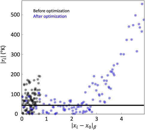
FIGURE 5. Absolute values of the residues as a function of the normalized distance for datapoints used to calculate gradients at time ∼75 min (latitude ∼80°) for the example shown on the right panels of Figure 4. Optimization results in reducing the homogeneity scales by a factor of ∼7. As a result, |xi − x0|β increases, updating the weights assigned to each datapoint, and subsequently modifying the calculated ∇lat, ∇long, and ∇t by −96, 97, −740%, respectively, while altering the distribution of the residues as a function of the normalized distance.
With the implementation of the least-squares gradient calculation approach validated via the synthetic example, we now turn to more realistic scenarios to test the ability of the software to determine the local dynamic of the ionosphere and thermosphere using GDC measurements. Figure 6A shows a frozen-in-time snapshot of the electron density as a function of geographic latitude and longitude from a three-dimensional TIEGCM simulation, featuring the Equatorial Ionization Anomaly (EIA). EIA is a dayside/dusk ionospheric feature that is formed from a phenomenon known as the Fountain/Appleton effect (Appleton, 1946). This phenomenon is a result of a vertical ion drift near the magnetic equator that is related to the E-region dynamo (Hanson and Moffett, 1966). This results in a concentration of plasma at ± 20° in magnetic latitude with a depletion of plasma at the magnetic equator primarily in the F-region (200–450 km) (Rishbeth, 2000). The EIA is in a highly collisional domain and is coupled with the thermosphere, but due to the lack of spatial and temporal resolutions from data collected in previous missions, there are unanswered questions to the exact coupling mechanisms in this region. Here, we employ simulations of the EIA using NCAR’s High-Resolution Thermosphere-Ionosphere-Electrodynamics General Circulation Model (HR-TIEGCM). HR-TIEGCM is a global 3D numerical model that can simulate the IT region from ∼97 km to ∼600 km with a longitude/latitude grid of 0.625 ° × 0.625 °, a vertical resolution of 0.25 of a scale height, and a timestep of 60 s (Qian et al., 2014; Dang et al., 2021). This temporal and spatial resolution is on par with what the GDC mission will be capable of capturing.
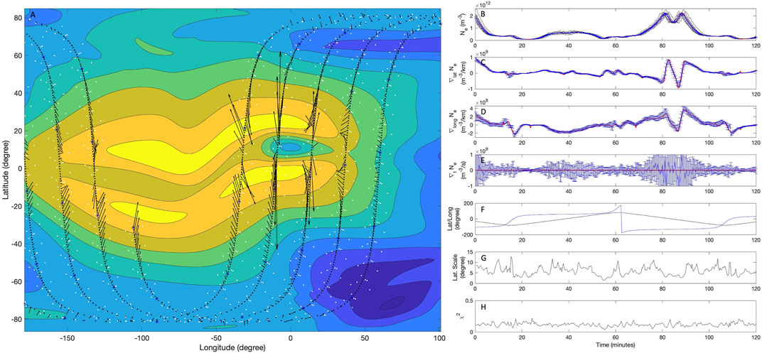
FIGURE 6. Results of the gradient calculation technique on simulated ionospheric electron density via TIEGCM. (A) 2d map showing the equatorial ionization anomaly, with gradient vectors calculated during GDC’s phase 1a. The continuous black lines shows the trajectory of the evaluation point. For reference, the white dots show trajectories of individual satellites, representing the size of the constellation. (B) time series results of the computations are shown in a similar format as those in Figure 3. 4% measurement noise has been added to the sampled data. Other settings include: Llat: 10°, Llong: 50°, Lt: 2,500 s, MaxT: 2 min; Measurement cadence: 20 s.
Our goal in this example is to evaluate the performance of LSGC-AS-LEO 1.0 to calculate the spatial gradients associated with the EIA using GDC data. In order to properly display the calculated gradients in the context of the two-dimensional image on Panel A, we briefly ignore the temporal variations of the electron density and assume that temporal gradients are zero at all locations. Upon running the software, the simulated data are imported and interpolated every 20 s along the trajectories of the GDC spacecraft during the first few hours of phase 1a. 4% measurement noise is then introduced to the data, which is comparable to the expected performance (i.e., 2% accuracy, and 1% precision) of GDC’s Atmospheric Electrodynamics probe for THERmal plasma (AETHER) instrument. The gradients are calculated with the initial homogeneity scales of Llat = 10°, Llong = 50°, and Lt = 2,500 s. Overplotted on the electron density map on Panel A is the trajectory of the evaluation point (the continuous black curve), as well as the spatial gradient vectors (black arrows). One can verify that the gradient vectors always point nearly perpendicular to the electron density contours. Shown on the right panels, in a similar format as those in Figure 3, are the electron densities seen by individual satellites (Panel B), the latitudinal (C), longitudinal (D), and temporal (E) gradients, latitude and longitude of the evaluation point (F) at the center of the constellation, Llat (G), and χ2 (H). While in Panel A gradient vectors are calculated and shown for about 5 GDC orbits through the simulated field, the right panels only show time series for the first 120 min (∼1.3 orbits) from the beginning of the interval starting at round −30° latitude and −106° longitude. The blue circles overplotted on the trajectory of the evaluation point in Panel A mark temporal timesteps of 10 min, allowing to compare the time series plots with the two-dimensional map in Panel A. The gradients are calculated accurately with the exception of the temporal gradients which suffer from very large error bars. The reason for these error estimates will be discussed later when visiting Figure 7. The spatial gradients shown in Panels C and D allow us to visualize the underlying electron density field without referring to the two-dimensional map on Panel A. For example, from the large negative longitudinal gradients around time 40 min, one could conclude that the electron density peak seen in Panel B at that time is due to a primarily longitudinal structure. This can indeed be confirmed by visiting Panel A and noting that observed electron density enhancement around time 40 min is due the constellation traversing along the eastern edge of the EIA at the longitude of ∼60° and the latitude range of −20 to +40°.
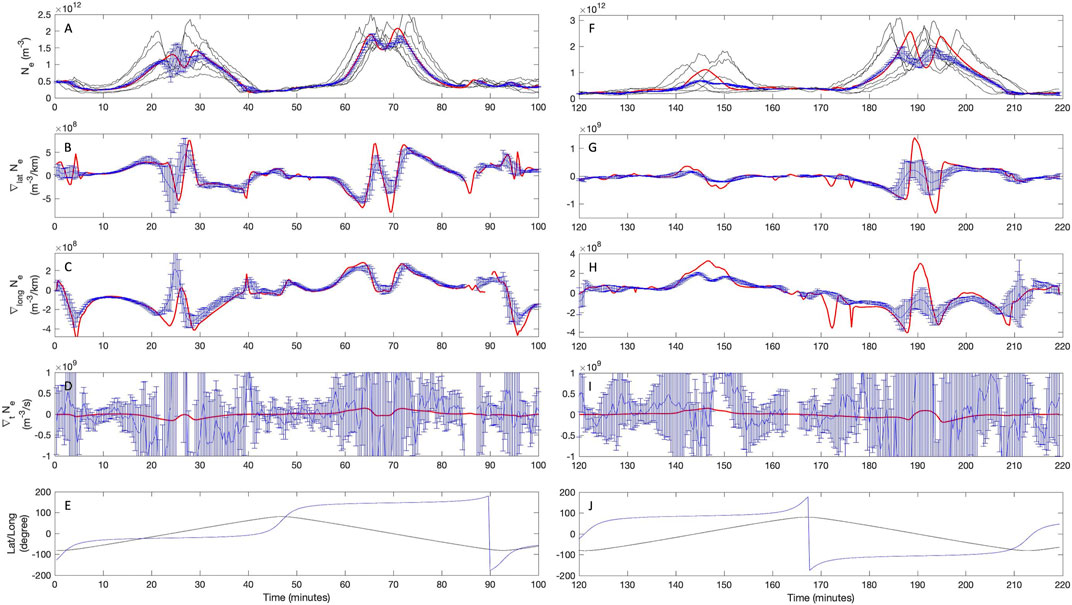
FIGURE 7. In a similar format as Figures 6B–F, the results of the gradient calculations on electron density but during the initial periods of GDC’s phases 2a (left) and 2b (right). The increased size of the constellation is evident in the top panels as the individual satellites measures increasingly different values.
In Figure 7 we repeat a similar test as that in Figure 6 while focusing on the constellation architecture at later phases of the mission. Here, the left panels correspond to the first 100 min of phase 2a and the panels on the right correspond to the beginning of the phase 2b. The figures show electron densities observed by individual satellites (Panel A and F), the calculated gradients (B–D and G–I), and the latitude and longitude of the evaluation point (F and J). In both examples we allow the simulated electron density field to evolve in time, such that the true temporal gradient are non-zero. At the beginning of phase 2a, it appears that the spatial gradients associated with the EIA are often properly captured. However, by the beginning of phase 2b, the size of the constellation has increased such the certain smaller scale features are no longer resolved, and at times the sharpest gradients are underestimated—e.g., around time 140–150 and 185–195 min. As a consequence of these errors, the estimated electron density at the evaluation point, at the center of the constellation, also deviate from the true values in Panel F. With respect to the temporal gradients, in both Panels D and J, the estimated values are significantly greater than true gradients and are accompanied by very large error bars, indicating that the estimates are likely not meaningful.
The difficulty in determining ∇tNe in this case arises from several factors which include: 1) the constellation architecture during the chosen phases of the mission, including the large (∼7 km/s) velocity of the satellites, that limits the duration of time over which a given spatial region is visited; 2) the ratio of the spatial gradients to ∇tNe at a given point; and 3) the relatively large measurement noise introduced to the samples. For example, consider the largest true temporal gradients in Figure 7D that reach a maximum of
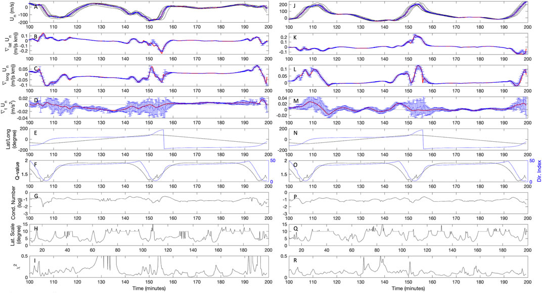
FIGURE 8. Results of the gradient computation on zonal (left) and meridional (right) neutral winds from TIEGCM simulations. 1% measurement noise has been added to the data sampled during the initial stages of the phase 1a. Other settings include: Llat: 10°, Llong: 20°, Lt: 500 s, MaxT: 3 min; Measurement cadence: 20 s.
In Figure 8 we return to the constellation geometry in phase 1a and evaluate the performance of the software in disentangling the spatial and temporal variability in a vector quantity: the zonal (U, shown on the left) and meridional (V, shown on the right) neutral winds as simulated by TIEGCM. Here, in order to demonstrate the ability of the approach to capture temporal gradients only 1% noise has been added to the simulated values. For reference, the expected performance of GDC’s neutral wind measurements by the Modular Spectrometer for Atmosphere and Ionosphere Characterization (MoSAIC) instrument is the accuracy and precision of no more than 4.5 m/s. With this level of measurement noise, all the gradients are determined with reasonably small error bars, including periods of non-zero ∇tUn and ∇tVn between times ∼120–150, as well as the most prominent variations of spatial gradients near the polar regions. While the specified 4.5 m/s accuracy of neutral wind measurement by the MoSAIC instrument translates to measurement noise levels as low as 2.25% in our example, an effective measurement noise of 1% or below is achievable by averaging multiple datapoints from MoSAIC that will be obtained within the 20-s measurement cadence used in our example shown in Figure 8. MoSAIC will provide independent samples of ion and neutral densities, temperatures, compositions, and velocities every two seconds or faster, providing a minimum of 10 samples within 20 s, providing the possibility to effectively reduce random measurement noise level by a factor of ∼3, to below 1%.
It is important to recognize that the ability of a mission like GDC to measure gradients relies on a reasonably good match between the spatiotemporal separation of the satellites and the phenomena being studied. Early phases of the mission are best for studying small-scale, sharp variations, and later phases are best for studying larger-scale, more gradual variations. As an example consider the simulated neutral temperature field shown in Figure 9A. The image shows variation of Tn in space at a fixed time, with the minimum and maximum values of ∼850 and 1200 K, respectively. For reference, the trajectory of the GDC constellation during the first orbit of phase 2b are also overplotted on the image. In the right panels of Figure 9, the gradients computed during phase 2b of the mission are shown to successfully capture the spatial variations of the underlying field. It should also be emphasized that, while the examples shown in Figures 3–9 demonstrate that the least-squares gradients calculation approach is a powerful tool capable of estimating the gradients of the IT parameters using GDC’s future measurements, the utilization of the approach is not necessarily trivial or free from limitations and caveats. For example, the performance of the algorithm currently relies on appropriate choices for several parameters, such as the homogeneity lengths, the determination of which may prove to be difficult in a real scenario. Further, for the approach to be applicable in a routine and robust manner, the sensitivity of the chosen parameter values needs to be studied. Such investigations will be the subject of future works.

FIGURE 9. (A) shows a snapshot of the neutral temperature from TIEGCM as a function of latitude and longitude. For reference, the trajectory of the center of the constellation and those of the individual satellites during the first orbit of phase 2b are also shown via the black line and white dots, respectively. (B–J) show results of the gradient computation for neutral temperature measurements at the beginning of phase 2b, subject to 2% measurement noise—that is MoSAIC’s expected accuracy and precision in determining the neutral gas temperature. Other settings include: Llat: 50°, Llong: 50°, Lt: 2,500 s, MaxT: 2.5 min, Measurement cadence: 20 s.
In preparation for the Geospace Dynamics Constellation mission, we have implemented the least-square gradient calculation approach described by De Keyser et al. (2007) and De Keyser (2008) in a open-source software LSGC-AS-LEO 1.0. Calculation of the gradients of the ionospheric and thermospheric parameters would allow to disentangle the spatial and temporal variability of the measured fields in an inherently quantitative manner. The approach that is implemented is flexible and, thus, highly suitable for GDC’s dynamic constellation architecture. Via a number of examples, and by utilizing synthetic and simulated IT fields, we have validated the performance of the software and demonstrated its power to explore GDC’s ability to resolve spatial and temporal structures that may exist in the ionosphere and the thermosphere. We have also established the usefulness of the software to evaluate suitability of various constellation geometries and assess the impact of measurement sensitivities on addressing GDC’s science objectives. For example, from the test cases discussed one may draw the following several conclusions: 1) computation of the temporal gradients of neutral and plasma variables, while are sensitive to the measurement noise level, are possible with GDC measurements; 2) The spatial gradients of the equatorial ionization anomaly can be reasonably resolved during phase 1 of the mission, while at the later phases the gradients are likely to be underestimated. On the other hand, in the presence of measurement noise, computing the gradients of the neutral temperature would likely be more difficult in the earliest phases of the mission due to the small gradients and large homogeneity lengths involved; 3) Gradients of the neutral wind can be well determined in the earliest phases of the mission even at the highest latitudes where the constellation skews in longitude.
We will continue to enhance the software in several directions. The future work will include further refinements to the optimization scheme and implementation of direction-dependent scaling for the homogeneity lengths, implementation of constrains (e.g., divergence free or curl free) in the algorithm for vector fields, enhancement of computation efficiency, and performing additional tests on simulated data to further probe GDC’s ability to address its science questions.
LSGC-AS-LEO v1 has been uploaded to Zenodo and can be found at https://doi.org/10.5281/zenodo.10685218. Further inquiries can be directed to the corresponding author.
All authors listed have made a substantial, direct, and intellectual contribution to the work and approved it for publication.
This work was funded by NASA’s Geospace Dynamics Constellation mission.
The authors declare that the research was conducted in the absence of any commercial or financial relationships that could be construed as a potential conflict of interest.
All claims expressed in this article are solely those of the authors and do not necessarily represent those of their affiliated organizations, or those of the publisher, the editors and the reviewers. Any product that may be evaluated in this article, or claim that may be made by its manufacturer, is not guaranteed or endorsed by the publisher.
Amm, O., and Viljanen, A. (1999). Ionospheric disturbance magnetic field continuation from the ground to the ionosphere using spherical elementary current systems. Earth, Planets Space 51, 431–440. doi:10.1186/bf03352247
Bard, C., and Dorelli, J. (2021). Neural network reconstruction of plasma space-time. Front. Astronomy Space Sci. 8, 732275. doi:10.3389/fspas.2021.732275
Blagau, A., and Vogt, J. (2019). Multipoint field-aligned current estimates with swarm. J. Geophys. Res. Space Phys. 124, 6869–6895. doi:10.1029/2018ja026439
Blagau, A., and Vogt, J. (2023). Swarmface: a python package for field-aligned currents exploration with swarm. Front. Astronomy Space Sci. 9, 1077845. doi:10.3389/fspas.2022.1077845
Burch, J., Moore, T., Torbert, R., and Giles, B. (2016). Magnetospheric multiscale overview and science objectives. Space Sci. Rev. 199, 5–21. doi:10.1007/s11214-015-0164-9
Chanteur, G. (1998). Spatial interpolation for four spacecraft: theory. ISSI Sci. Rep. Ser. 1, 349–370.
Dang, T., Zhang, B., Lei, J., Wang, W., Burns, A., Liu, H.-l., et al. (2021). Azimuthal averaging–reconstruction filtering techniques for finite-difference general circulation models in spherical geometry. Geosci. Model Dev. 14, 859–873. doi:10.5194/gmd-14-859-2021
Darrouzet, F., De Keyser, J., Décréau, P., Lemaire, J., and Dunlop, M. (2006). Spatial gradients in the plasmasphere from cluster. Geophys. Res. Lett. 33. doi:10.1029/2006gl025727
De Keyser, J. (2008). Least-squares multi-spacecraft gradient calculation with automatic error estimation. Ann. Geophys. (Copernic. GmbH) 26, 3295–3316. doi:10.5194/angeo-26-3295-2008
De Keyser, J., Darrouzet, F., Dunlop, M., and Décréau, P. (2007). Least-squares gradient calculation from multi-point observations of scalar and vector fields: methodology and applications with cluster in the plasmasphere. Ann. Geophys. (Copernic. GmbH) 25, 971–987. doi:10.5194/angeo-25-971-2007
Denton, R., Torbert, R., Hasegawa, H., Dors, I., Genestreti, K., Argall, M., et al. (2020). Polynomial reconstruction of the reconnection magnetic field observed by multiple spacecraft. J. Geophys. Res. Space Phys. 125, e2019JA027481. doi:10.1029/2019ja027481
Denton, R. E., Liu, Y.-H., Hasegawa, H., Torbert, R. B., Li, W., Fuselier, S., et al. (2022). Polynomial reconstruction of the magnetic field observed by multiple spacecraft with integrated velocity determination. J. Geophys. Res. Space Phys. 127, e2022JA030512. doi:10.1029/2022ja030512
Dunlop, M., Dong, X.-C., Wang, T.-Y., Eastwood, J., Robert, P., Haaland, S., et al. (2021a). Curlometer technique and applications. J. Geophys. Res. Space Phys. 126, e2021JA029538. doi:10.1029/2021ja029538
Dunlop, M. W., and Lühr, H. (2020). Ionospheric multi-spacecraft analysis tools: approaches for deriving ionospheric parameters. Berlin, Germany: Springer Nature.
Dunlop, M. W., Wang, T., Dong, X., Haarland, S., Shi, Q., Fu, H., et al. (2021b). Multispacecraft measurements in the magnetosphere. Magnetos. Sol. Syst., 637–656. doi:10.1002/9781119815624.ch40
Escoubet, C., Fehringer, M., and Goldstein, M. (2001). <i&gt;Introduction&lt;/i&gt;The Cluster mission. Ann. Geophys. (Copernic. GmbH) 19, 1197–1200. doi:10.5194/angeo-19-1197-2001
Fiori, R. A. (2020). Spherical cap harmonic analysis techniques for mapping high-latitude ionospheric plasma flow—application to the swarm satellite mission. Ionos. Spacecr. Analysis Tools Approaches Deriving Ionos. Param., 189–218. doi:10.1007/978-3-030-26732-2_9
Friis-Christensen, E., Lühr, H., Knudsen, D., and Haagmans, R. (2008). Swarm–an earth observation mission investigating geospace. Adv. Space Res. 41, 210–216. doi:10.1016/j.asr.2006.10.008
Hanson, W., and Moffett, R. (1966). Lonization transport effects in the equatorial f region. J. Geophys. Res. 71, 5559–5572. doi:10.1029/jz071i023p05559
Paschmann, G., and Daly, P. W. (1998). Analysis methods for multi-spacecraft data. ISSI Sci. Rep. Ser. 1, 1608–280x.
Qian, L., Emery, B. A., Foster, B., Lu, G., Maute, A., Richmond, A. D., et al. (2014). The NCAR TIE-GCM: a community model of the coupled thermosphere/ionosphere system,” in Model. ionosphere–thermosphere Syst. Eds., Editor J. Huba, R. Schunk, and G. Khazanov: John Wiley, 73–83. doi:10.1002/9781118704417.ch7
Rishbeth, H. (2000). The equatorial f-layer: progress and puzzles. Ann. Geophys. 18, 730–739. doi:10.1007/s005850000221
Ritter, P., and Lühr, H. (2006). Curl-b technique applied to swarm constellation for determining field-aligned currents. Earth, planets space 58, 463–476. doi:10.1186/bf03351942
Ritter, P., Lühr, H., and Rauberg, J. (2013). Determining field-aligned currents with the swarm constellation mission. Earth, Planets Space 65, 1285–1294. doi:10.5047/eps.2013.09.006
Robert, P., Dunlop, M. W., Roux, A., and Chanteur, G. (1998). Accuracy of current density determination. Analysis methods Spacecr. data 398, 395–418.
Shen, C., and Dunlop, M. (2023). Field gradient analysis based on a geometrical approach. J. Geophys. Res. Space Phys. 128, e2023JA031313. doi:10.1029/2023ja031313
Shen, C., Rong, Z., and Dunlop, M. (2012a). Determining the full magnetic field gradient from two spacecraft measurements under special constraints. J. Geophys. Res. Space Phys. 117. doi:10.1029/2012ja018063
Shen, C., Rong, Z., Dunlop, M., Ma, Y., Li, X., Zeng, G., et al. (2012b). Spatial gradients from irregular, multiple-point spacecraft configurations. J. Geophys. Res. Space Phys. 117. doi:10.1029/2012ja018075
Shen, C., Zhang, C., Rong, Z., Pu, Z., Dunlop, M. W., Escoubet, C. P., et al. (2021a). Nonlinear magnetic gradients and complete magnetic geometry from multispacecraft measurements. J. Geophys. Res. Space Phys. 126, e2020JA028846. doi:10.1029/2020ja028846
Shen, C., Zhou, Y., Ma, Y., Wang, X., Pu, Z., and Dunlop, M. (2021b). A general algorithm for the linear and quadratic gradients of physical quantities based on 10 or more point measurements. J. Geophys. Res. Space Phys. 126, e2021JA029121. doi:10.1029/2021ja029121
Torbert, R. B., Dors, I., Argall, M. R., Genestreti, K., Burch, J., Farrugia, C. J., et al. (2020). A new method of 3-d magnetic field reconstruction. Geophys. Res. Lett. 47, e2019GL085542. doi:10.1029/2019gl085542
Vogt, J., Albert, A., and Marghitu, O. (2009). Analysis of three-spacecraft data using planar reciprocal vectors: methodological framework and spatial gradient estimation. Ann. Geophys. 27, 3249–3273. doi:10.5194/angeo-27-3249-2009
Vogt, J., Blagau, A., and Pick, L. (2020). Robust adaptive spacecraft array derivative analysis. Earth Space Sci. 7, e2019EA000953. doi:10.1029/2019ea000953
Vogt, J., Sorbalo, E., He, M., and Blagau, A. (2013). Gradient estimation using configurations of two or three spacecraft. Ann. Geophys. 31, 1913–1927. doi:10.5194/angeo-31-1913-2013
Keywords: multi-point in-situ measurements, satellite constellation, Geospace Dynamics Constellation (GDC), ionospheric dynamics, gradient calculation
Citation: Akbari H, Rowland D, Coleman A, Buynovskiy A and Thayer J (2024) Gradient calculation techniques for multi-point ionosphere/thermosphere measurements from GDC. Front. Astron. Space Sci. 11:1231840. doi: 10.3389/fspas.2024.1231840
Received: 31 May 2023; Accepted: 09 February 2024;
Published: 29 February 2024.
Edited by:
David Knudsen, University of Calgary, CanadaReviewed by:
Joachim Vogt, Jacobs University Bremen, GermanyCopyright © 2024 Akbari, Rowland, Coleman, Buynovskiy and Thayer. This is an open-access article distributed under the terms of the Creative Commons Attribution License (CC BY). The use, distribution or reproduction in other forums is permitted, provided the original author(s) and the copyright owner(s) are credited and that the original publication in this journal is cited, in accordance with accepted academic practice. No use, distribution or reproduction is permitted which does not comply with these terms.
*Correspondence: Hassanali Akbari, aGFzc2FuYWxpLmFrYmFyaUBuYXNhLmdvdg==
Disclaimer: All claims expressed in this article are solely those of the authors and do not necessarily represent those of their affiliated organizations, or those of the publisher, the editors and the reviewers. Any product that may be evaluated in this article or claim that may be made by its manufacturer is not guaranteed or endorsed by the publisher.
Research integrity at Frontiers
Learn more about the work of our research integrity team to safeguard the quality of each article we publish.