Uncovering the heterogeneity of a solar flare mechanism with mixture models

The physics of solar flares occurring on the Sun is highly complex and far from fully understood. However, observations show that solar eruptions are associated with the intense kilogauss fields of active regions, where free energies are stored with field-aligned electric currents. With the advent of high-quality data sources such as the Geostationary Operational Environmental Satellites (GOES) and Solar Dynamics Observatory (SDO)/Helioseismic and Magnetic Imager (HMI), recent works on solar flare forecasting have been focusing on data-driven methods. In particular, black box machine learning and deep learning models are increasingly being adopted in which underlying data structures are not modeled explicitly. If the active regions indeed follow the same laws of physics, similar patterns should be shared among them, reflected by the observations. Yet, these black box models currently used in the literature do not explicitly characterize the heterogeneous nature of the solar flare data within and between active regions. In this paper, we propose two finite mixture models designed to capture the heterogeneous patterns of active regions and their associated solar flare events. With extensive numerical studies, we demonstrate the usefulness of our proposed method for both resolving the sample imbalance issue and modeling the heterogeneity for rare energetic solar flare events.

1 Introduction

Solar flares originate from explosions of magnetic energy caused by tangling, crossing, or reorganizing of magnetic field lines. Flares can last from minutes to hours and can disrupt space–Earth radio communications, increasing satellite drag when reaching certain thresholds. An example is the October 2003 superstorm event, where the Sun unleashed powerful solar flares and coronal mass ejections that impacted the space environment of Earth. In late 28 October 2003, the Sun produced the “Halloween Storms of 2003,” as dubbed by NASA (NASA, 2003), whose impact on Earth caused airplanes to be rerouted, impacted satellite systems, and created power outages in Sweden. The Solar and Heliospheric Observatory (SOHO) was temporarily overwhelmed during the solar onslaught.

The energy release mechanism of solar flares is yet to be fully characterized. Observations have established that they are strongly associated with nonpotential magnetic fields, which store necessary free energy (Chen et al., 2019). Most flares originate from localized intense kilogauss photospheric fields, which produce active regions (ARs). The accurate photospheric measurement of these fields has been greatly enhanced with the Helioseismic and Magnetic Imager (HMI) instrument on the Solar Dynamics Observatory (SDO) launched in February 2010 (Schou et al., 2012). The HMI provides high-quality data in the form of high-cadence, high-resolution vector magnetograms, which span the entire solar disk. These data are saved at a 12-min cadence. The analysis and storage are subdivided into HMI Active Region Patches (HARPs), which are cutouts of the magnetograms. Time series of HARP data track the evolution of each AR from the time it appears until its disappearance, either by emergence/dispersion or rotating on/off the visible disk. From the 2D HARP data field, scalar quantities referred to as Space-weather HARP (or SHARP) are calculated, which includes 16 indices computed from the full 3-component vector magnetic field. These parameters are automatically calculated for HARPs and made available, along with the HARP magnetogram data, by the Joint Science Operations Center (JSOC) located at Stanford University (Bobra et al., 2014).

Machine learning (ML) algorithms have become increasingly common among space weather practitioners. At first, the line-of-sight (LOS) component of the photospheric magnetic field measured using the Michelson Doppler Imager (MDI) instrument (launched in 1995 as part of the Solar and Heliospheric Observatory) was used by several research groups to forecast solar flares using ML models (Song et al., 2009; Yu et al., 2009; Yuan et al., 2010; Ahmed et al., 2013; Huang et al., 2018). Later studies used SDO/HMI data, which provide the full vector magnetic field data with twice the spatial resolution and eight times the data cadence as the MDI. Bobra and Couvidat (2015) used the support vector machine (SVM) trained with SHARP parameters for active region classification tasks (Bobra et al., 2014; Barnes et al., 2016; Leka et al., 2018; Camporeale, 2019). Recently, deep learning models such as long short-term memory (LSTM) networks, recurrent neural networks (RNNs), and convolutional neural networks (CNNs) have also been adopted to exploit the correlated structure among the time series data (Chen et al., 2019; Liu et al., 2019; Jiao et al., 2020; Wang et al., 2020; Landa and Reuveni, 2022). While these black box models have enjoyed predictive performance gains, their limitation is typically not being able to shed light on the underlying structures of the raw data, which can be utilized to gain new insights into the physics of solar flares.

Chen et al. (2019) built an LSTM neural network classifier with the parameters of HMI/SHARP patches from 1 May 2010 to 20 June 2018 as their covariate data. For the corresponding response variables, they took advantage of the data from the National Oceanic and Atmospheric Administration (NOAA) Geostationary Operational Environmental Satellites (GOES) flare list during the same time period (Garcia, 1994). GOES flare data are provided both as a time series of soft X-ray intensities and a list of flare events, including start time, peak time, and peak X-ray intensity, recorded by space weather satellites. The GOES satellites are managed by the NOAA, and its spacecraft is located at a height of approximately 35,800 km, providing an uninterrupted view of the Sun. The main objective of GOES is collecting infrared radiation and solar reflection from Earth’s surface (Garcia, 1994).

The work in this paper closely follows the above data framework laid out by Chen et al. (2019), with some differences. To make the task of binary classification manageable with an LSTM network, Chen et al. (2019) considered only the B and M/X flares and excluded the prevalent C flare, because their intensities straddle between the range of strong and weak flares, making the classification harder. In contrast, here, we account for all data, including the C flares, as we wish to model the intensities of the flares as continuous values to closely resemble the observed data. Moreover, Chen et al. (2019) treated SDO/HMI stream data as time series where ARs are recorded from their initial appearance to disappearances. Here, we consider each flare only at its peak time (at the highest intensity). As such, our data are not time series and should be considered a collection of discrete events occurring at different time points.

In our work, we are interested in the shared properties of active regions. Studies on the space weather have applied machine learning methods to classify active regions (Nguyen et al., 2004; Colak and Qahwaji, 2008; Maloney and Gallagher, 2018; Smith et al., 2018). The methods used in these works include support vector machines, random forest classification, K-nearest neighbor classification, and neural networks, which do not explicitly take into account the rich statistical structure of the data. In addition, these black box models typically do not yield more insights into the underlying data structure. Most recently, Baeke et al. (2023) applied unsupervised learning methods such as K-means and the Gaussian mixture model to cluster active regions. However, the authors clustered active regions on the data covariates. Our work in this paper clusters active regions based on the interaction between the response and the covariate of the data. We believe model-based clustering at this level would be more interesting and meaningful to space weather scientists.

It is scientifically reasonable to believe that solar flares across the Sun’s active regions follow similar laws of physics, and so SHARP parameters of active regions should share some common data patterns. Nevertheless, to the best of our knowledge, the heterogeneous nature of solar flare data has not been characterized or exploited in the space weather literature. Our contribution in this paper, which marks its difference from other works, is to apply mixture models to detect and elucidate the heterogeneous patterns of active regions. The idea of mixture modeling is to describe a complicated data distribution as a weighted combination of simpler distributions (Titterington et al., 1985; McLachlan and Peel, 2000). They are especially useful in a setting where data naturally come from a number of “homogeneous” subgroups within a population. For example, human height data can be considered a mixture of two subgroups, male and female. Mixture models have played a central role in machine learning and statistics, with broad applications, including bioinformatics, natural language and speech processing, and computer vision (Bishop, 2006). A challenge of mixture modeling is the technical difficulty in parameter estimation. Finding the maximum likelihood estimates of the model often involves solving a non-convex optimization problem (Bishop, 2006). In practice, maximum likelihood estimation via the expectation-maximization (EM) algorithm has been the workhorse for these models (Dempster et al., 1977). In the solar flare prediction problem, different active regions across the surface of the Sun seem to share certain common characteristics and are, thus, a good candidate for mixture modeling. We propose two types of mixture models. The first model is designed to characterize the heterogeneous pattern of active regions, as mentioned. The second model goes further and allows for the heterogeneity of individual flare events within an active region. As demonstrated later, using mixture models for active regions does improve the predictive performance and confirms the validity of the empirical observation that active regions share similar patterns. The second proposed mixture model further improves the performance, albeit marginally, implying that heterogeneous patterns are not only restricted to active regions but also potentially extend to flare events within action regions. Since energetic solar flares are extremely rare events compared to low-energy flares, which occur orders of magnitude more frequently, statistical inference for this type of data needs to address the data imbalance issue (Bobra and Couvidat, 2015). So, another contribution of this paper is showing how to deal with the imbalance problem using the expectation-maximization framework.

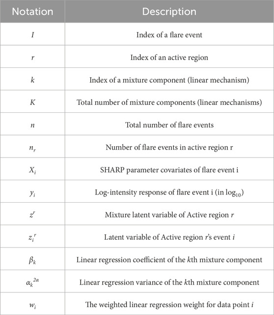
The paper is organized as follows: Section 2 describes the data preprocessing procedure; Section 3 proposes two types of mixture models designed to capture the heterogeneous properties of solar flare data; Section 4 provides the detailed data analysis results and interpretation; and Section 5 concludes and briefly touches on future work. Table 1 lists all notations used within the text.

TABLE 1

TABLE 1. Summary of notations used in the paper.

2 Data preprocessing and feature selection

2.1 Raw data

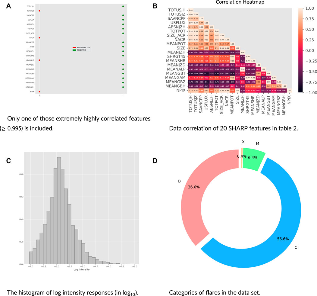
For response variables, we take advantage of the recorded log intensities of flare events in the GOES data set (Garcia, 1994) ranging from 2 June 2010 to 29 December 2018. The flare events are recorded at their peak time (time at the highest flare intensity). Although the theoretical distribution of the flare events should be a power law distribution, the observed distribution is different from the theoretical distribution because flares in lower-energy levels are lost in the background and go undetected (Jiao et al., 2020). In this paper, we focus on the observed information. By scientific convention, solar flares belong to category B if their log intensity (log₁₀) is within (−∞, −6), category C if [−6, −5), category M if [−5, −4), and category X if (−4, ∞). Figure 1D shows that the M/X flare events are far fewer than B/C. The data imbalance issue is addressed in Section 3.1.

FIGURE 1

FIGURE 1. Description of the HMI/SDO SHARP dataset.

For covariates/features, we consider SHARP data (Schou et al., 2012) from 860 HARPs during the same time period (2 June 2010 to 29 December 2018). Approximately 7,000 HARPs are observed, many occurring without flares. From these, to maintain the quality of the data, we down-select the HARPs to a group of 860 based on the criteria that 1) the longitude of the HARP should be within the range of ±68° from the central meridian of the Sun to avoid projection effects (Bobra and Couvidat, 2015; Chen et al., 2019) and 2) the missing SHARP parameters should be fewer than 5% of all in the HARP to make sure that the missing data are not significantly large to cause any bias in model training.

For this type of data, an important practical goal of any model is to forecast the future flare intensity, given an observed value of SHARP parameters. As such, for each point in our dataset, we match the corresponding SHARP covariates with the GOES flare list (response variable) at the time point that is equal to the peak time subtracted by Δt, where Δt is the prediction time window and can take values in {6, 12, 24, 36, 48} h.

2.2 Feature selection and preprocessing procedure

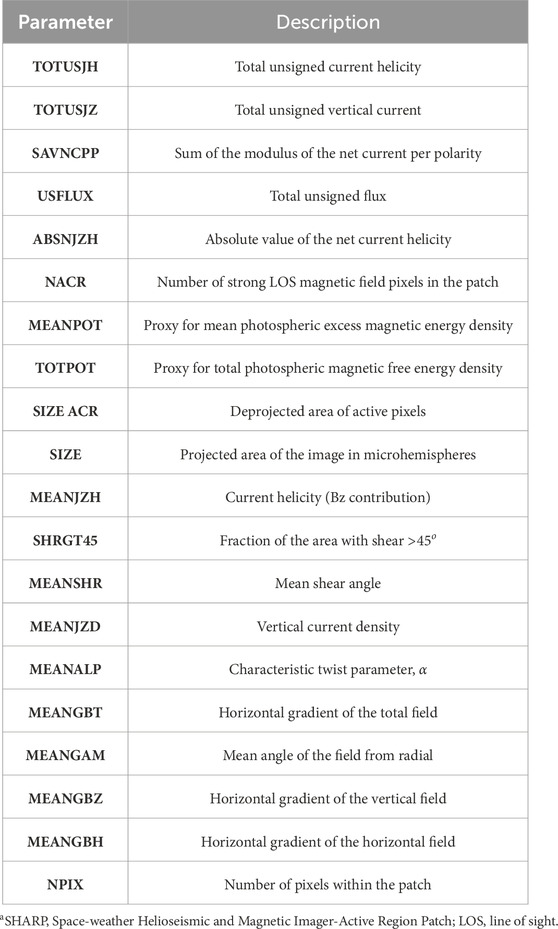
All covariates in the raw data are shown in Table 2. These are the same features used by Chen et al. (2019) and Bobra and Couvidat (2015). However, we only use a subset because our correlation analysis showed that some features are extremely highly correlated. Specifically, TOTUSJH/TOTUSJZ (0.9959), SIZE_ACR/NACR (0.9999), SHRGT45/MEANSHR (0.9969), and SIZE/NPIX (0.9999) are extremely highly correlated. For each of these features, we keep one feature and leave out the other. After removal, we are left with 16 covariates: TOTUSJH, SAVNCPP, USFLUX, ABSNJZH, TOTPOT, SIZE_ACR, MEANPOT, SIZE, MEANJZH, SHRGT45, MEANJZD, MEANALP, MEANGBT, MEANGAM, MEANGBZ, and MEANGBH. Their correlation matrix is displayed in Figure 1B.

TABLE 2

TABLE 2. List of SHARP parameters and their brief descriptions.

A key aspect of our models is modeling the flare intensities by ARs. Consequently, we need to ensure similar sets of ARs in both training and testing. To facilitate this, we randomly split data into a training set and testing set, the latter containing 20% of the total across all the ARs with two or more events. For those with only one event, we flip a biased coin with probability 0.2, assigning to the testing set if the result was true and, otherwise, to the training set. This random split scheme guarantees a fair representation of each AR in both the training set and testing set. Each feature in the training set was then standardized to have a zero mean and a standard deviation of one. We used these parameters to normalize the testing set. Additionally, we further randomly divided the training set by ARs into a sub-train set and a validation set, with the latter equal to 20% of the original set. We used this validation set for the model selection process discussed in Section 4.

3 Methodology

In this section, we describe our methodology for modeling the solar flare data described in the previous section. We begin by discussing a strategy to handle the data imbalance issue because space weather practitioners are mostly interested in catastrophic flare events (M/X), which occur less frequently than weak (B/C class) flares. Then, we apply mixture models to characterize the heterogeneity of solar flare mechanisms. Specifically, we describe the mixture models, mixture model over active regions (MM-R) and mixture model over flare events (MM-H), which characterize the heterogeneous patterns among active regions, with MM-H an extension of MM-R.

3.1 Approach to dealing with the data imbalance issue

Weighted likelihood and weighted maximum likelihood estimation (MLE) have been used in the literature for robust estimations, especially when outliers exist in the data (Carroll and Pederson, 1993; Field and Smith, 1994; Markatou et al., 1998). The idea is to down-weight the outlier data points so that they do not deteriorate the performance of the model too much. A similar principle can be applied here to handle the imbalance problem, i.e., down-weighting the “majority” data points and/or up-weighting the “minority” points.

To illustrate, we consider a simple example of a standard linear regression setting. Assume that the response y_i given covariate X_i follows the normal distribution $y_i|X_i\sim N(X_i^T\beta ,1),i=1,\dots ,n$, where β is the linear regression coefficient. The least squares estimate for β is given by $\widehat{\beta }={\text{arg\hspace{0.17em}max}}_{\beta }{\sum }_{i=1}^n-{(y_i-X_i^T\beta )}^2$. With highly imbalanced data like the solar flare data given in Section 2, standard linear regression would not work well, and weighted linear regression may be used instead. In that case, we need to calculate the weighted estimator $\tilde{\beta }={\text{arg\hspace{0.17em}max}}_{\beta }{\sum }_{i=1}^n-w_i\cdot {(y_i-X_i^T\beta )}^2$ for known weights w_i that may depend on the data. Moving beyond this simple example, the modeling we propose in the next sections is based on mixture models. Consider a simplified generative model as follows:

$y_i|X_i,z_i=k\sim \text{N}\left(y_i|X_i^T{\beta }_k,{\sigma }_k^2\right),k=1,\dots ,K,i=1,\dots ,n,$

where K denotes the number of mixture components and z_i is a categorical variable with P (z_i = k) = π_k for all k; ∑_kπ_k = 1. Applying the weighted likelihood idea, we aim to find the optimizer ${\text{arg\hspace{0.17em}max}}_{\theta }{\sum }_{i=1}^n{w}_i\cdot \log p(y_i|X_i,\theta )$, where $\theta ≔{\{{\beta }_k,{\sigma }_k^2,{\pi }_k\}}_1^K$. Recall that the original log-likelihood is $l(\theta )≔{\sum }_{i=1}^n\log p(y_i|X_i,\theta )$. For mixture models, it is not straightforward to directly maximize l(θ). The expectation-maximization (EM) algorithm is needed (Dempster et al., 1977). Typically, the EM algorithm works with the logarithm of the complete data likelihood, which is defined as $l(\pi ,\beta ,{\sigma }^2)≔{\sum }_{k=1}^K{\sum }_{i=1}^n\mathbb{1}(z_i=k)\cdot \left[\log {\pi }_k+\log \text{N}(y_i|X_i^T{\beta }_k,{\sigma }_k^2)\right]$. In the E-step, the EM algorithm computes ${\tau }_{i,k}≔p(z_i=k|X_i,y_i)≔\frac{{\pi }_k\text{N}(y_i|X_i^T{\beta }_k,{\sigma }_k^2)}{{\sum }_{j=1}^K{\pi }_j\text{N}(y_i|X_i^T{\beta }_j,{\sigma }_j^2)}$, k = 1, … , K; then, it maximizes the expected complete log-likelihood, ${\text{arg\hspace{0.17em}max}}_{\beta ,{\sigma }^2,\pi }Q(\beta ,{\sigma }^2,\pi )≔{\text{arg\hspace{0.17em}max}}_{\beta ,{\sigma }^2,\pi }{\sum }_{i=1}^n{\sum }_{k=1}^K{\tau }_{i,k}\cdot \left[\text{log}{\pi }_k+\log \text{N}(y_i|X_i^T{\beta }_k,{\sigma }_k^2)\right]$, in the M-step. That yields ${\widehat{\pi }}_k=\frac{{\sum }_{i=1}^n{\tau }_{ik}}{n}$ and ${\widehat{\mu }}_k=\frac{{\sum }_{i=1}^n{\tau }_{i,k}{X}_i}{{\sum }_{i=1}^n{\tau }_{i,k}}$ and ${\widehat{\sigma }}_k^2=\frac{{\sum }_{i=1}^n{\tau }_{ik}\cdot {(X_i-{\widehat{\mu }}_k)}^2}{{\sum }_{i=1}^n{\tau }_{ik}}$; k = 1, …, K.

To adapt the EM framework to find the MLE for the weighted likelihood, we note that under the EM algorithm, the log-likelihood is lower-bounded by the expected complete log-likelihood, i.e., l(θ) ≥ Q(θ), and by optimizing the lower bound Q(θ), the EM algorithm yields the (local) maximum of the likelihood l(θ) (Bishop, 2006). Under the weighted likelihood setting, we can also find a lower bound as follows:

$\begin{array}{ll}\hfill & {\displaystyle \sum _{i=1}^n}{w}_i\log p\left(y_i|X_i,\theta \right)\hfill \\ \hfill & ={\displaystyle \sum _{i=1}^n}{w}_i\log {\displaystyle \sum _{k=1}^K}p\left(y_i,z_i=k|X_i,\theta \right)\hfill \\ \hfill & ={\displaystyle \sum _{i=1}^n}{w}_i\cdot \log \left[{\displaystyle \sum _{k=1}^K}q\left(z_i=k\right)\cdot \frac{p\left(y_i,z_i=k|X_i,\theta \right)}{q\left(z_i=k\right)}\right]\hfill \\ \hfill & \ge {\displaystyle \sum _{i=1}^n}{w}_i\cdot {\displaystyle \sum _{k=1}^K}q\left(z_i=k\right)\log \left(\frac{p\left(y_i,z_i=k|X_i,\theta \right)}{q\left(z_i=k\right)}\right).\hfill \end{array}$

The last inequality is due to Jensen’s inequality. Since the logarithm is a concave function, and ${\sum }_{k=1}^{k}q(z_i=k)=1$, we moved the log inside and left q outside. Here, we can follow the usual EM procedure to find the optimal q(z). The E-step sets $q(z_i=k)=\mathbb{P}(z_i=k|X_i,y_i)$, and then, the M-step maximizes the subsequent expression. Therefore, we observe that the weighted log-likelihood is bounded below by the weighted expected complete log-likelihood. In other words, to find the weighted log-likelihood estimator with the EM framework, we can optimize the lower bound ${\sum }_{i=1}^n{\sum }_{k=1}^K{w}_i\cdot {\tau }_{i,k}\cdot \left[\text{log}{\pi }_k+\log \text{N}(y_i|X_i^T{\beta }_k,{\sigma }_k^2)\right]$. Moreover, since w_i (⋅) is a known weight function, if we ensure that 0 < w_i ≤ C < ∞ for all i for some constant C free of parameters, then, by noting that log  π_k < 0, we have

$\begin{array}{l}\hfill \begin{array}{cc}\hfill & {\displaystyle \sum _{i=1}^n}{\displaystyle \sum _{k=1}^K}{w}_i\cdot {\tau }_{i,k}\cdot \left[\text{log}{\pi }_k+\log \text{N}(y_i|X_i^T{\beta }_k,{\sigma }_k^2)\right]\hfill \\ \hfill & ={\displaystyle \sum _{i=1}^n}{\displaystyle \sum _{k=1}^K}{\tau }_{i,k}\cdot \left[w_i\cdot \text{log}{\pi }_k+w_i\log \text{N}(y_i|X_i^T{\beta }_k,{\sigma }_k^2)\right]\hfill \\ \hfill & \ge {\displaystyle \sum _{i=1}^n}{\displaystyle \sum _{k=1}^K}{\tau }_{i,k}\cdot \left[C\cdot \text{log}{\pi }_k+w_i\log \text{N}(y_i|X_i^T{\beta }_k,{\sigma }_k^2)\right].\hfill \end{array}\end{array}$

Because ${\sum }_{k=1}^K{\pi }_k=1$, it is easy to derive that

$\begin{array}{ll}\hfill & {\text{argmax\hspace{0.17em}}}_{\beta ,{\sigma }^2,\pi }{\displaystyle \sum _{i=1}^n}{\displaystyle \sum _{k=1}^K}{\tau }_{i,k}\cdot \left[C\cdot \text{log}{\pi }_k+w_i\log \text{N}\left(y_i|X_i^T{\beta }_k,{\sigma }_k^2\right)\right]\hfill \\ \hfill & ={\text{argmax\hspace{0.17em}}}_{\beta ,{\sigma }^2,\pi }{\displaystyle \sum _{i=1}^n}{\displaystyle \sum _{k=1}^K}{\tau }_{i,k}\cdot \left[\text{log}{\pi }_k\right.\hfill \\ \hfill & \left.+w_i\log \text{N}\left(y_i|X_i^T{\beta }_k,{\sigma }_k^2\right)\right].\hfill \end{array}$

Therefore, the above expression is the lower bound of the weighted complete log-likelihood, and optimizing it, in turn, increases the data likelihood. The final expression is the lower bound to be optimized for our mixture models, which is proposed in the subsequent sections. The justification of the algorithm comes from the fact that the EM-based inference algorithm will converge to a local maximum of the weighted likelihood function (Wu, 1983).

3.2 Dealing with the sample imbalance problem: weighting schemes

In this section, let w_i be denoted by w (y_i) to emphasize the fact that the weights only depend on y_i(s). By scientific convention, the log intensity is (in log₁₀) y_i ∈ (−∞, −6) for flare category B, y_i ∈ [−6, −5) for flare category C, y_i ∈ [−5, −4) for flare category M, and y_i ∈ (−4, ∞) for flare category X. We propose the following scheme for w (y_i):

$w\left(y_i\right)=\left\{\begin{array}{cc}\frac{1}{{\displaystyle \sum _{i=1}^n}\mathbb{1}\left(y_i\ge -4\right)/n}\hfill & \text{\hspace{0.17em}if\hspace{0.17em}}{y}_i\ge -4\hfill \\ \frac{1}{{\displaystyle \sum _{i=1}^n}\mathbb{1}\left(-5\le y_i<-4\right)/n}\hfill & \text{\hspace{0.17em}if\hspace{0.17em}}-5\le y_i<-4\hfill \\ \frac{1}{{\displaystyle \sum _{i=1}^n}\mathbb{1}\left(-6\le y_i<-5\right)/n}\hfill & \text{\hspace{0.17em}if\hspace{0.17em}}-6\le y_i<-5\hfill \\ \frac{1}{{\displaystyle \sum _{i=1}^n}\mathbb{1}\left(y_i<-6\right)/n}\hfill & \text{\hspace{0.17em}if\hspace{0.17em}}{y}_i<-6\hfill \end{array}\right..$

Note that as n → ∞, by the strong law of large numbers,

$w\left(y\right)\stackrel{a.s.}{\to }\left\{\begin{array}{cc}\frac{1}{{\int }_{-4}^{\infty }{p}_0\left(y\right)dy}\hfill & \text{\hspace{0.17em}if\hspace{0.17em}}y\ge -4\hfill \\ \frac{1}{{\int }_{-5}^{-4}{p}_0\left(y\right)dy}\hfill & \text{\hspace{0.17em}if\hspace{0.17em}}-5\le y<-4\hfill \\ \frac{1}{{\int }_{-6}^{-5}{p}_0\left(y\right)dy}\hfill & \text{\hspace{0.17em}if\hspace{0.17em}}-6\le y<-5\hfill \\ \frac{1}{{\int }_{-\infty }^{-6}{p}_0\left(y\right)dy}\hfill & \text{\hspace{0.17em}if\hspace{0.17em}}y<-6\hfill \end{array}\right.,$

where p₀y) is the marginal distribution of y. The justification for choosing w(y) this way is as follows. As the number of data points goes to infinity, and it is assumed that (X, y) follows the “true” distribution p₀ (X, y), by the law of large numbers, the weighted score function becomes

$\begin{array}{ll}\hfill & \frac{1}{n}{\displaystyle \sum _{i=1}^n}w\left(y_i\right)\log p\left(y_i|X_i,\theta \right)\hfill \\ \hfill & \stackrel{a.s.}{\to }\int w\left(y\right)\log p\left(y|x,\theta \right)p_0\left(x,y\right)dxdy\hfill \\ \hfill & =\int w\left(y\right)\cdot \left(\int \log p\left(y|x,\theta \right)p_0\left(x|y\right)dx\right)\cdot p_0\left(y\right)dy.\hfill \end{array}$

r (y, θ)≔∫ log  p (y|x, θ) p₀ (x|y)dx and I_B≔(−∞, −6), I_C≔[−6, −5), I_M≔[−5, −4), I_X≔[−4, ∞) are defined. These intervals correspond to the scientific thresholds of flare categories B, C, M, and X, respectively. As the number of data points goes to infinity, the weighted log-likelihood function can now be written as

$\begin{array}{l}\hfill \begin{array}{cc}\hfill & \int w(y)\log p(y|x,\theta )p_0(x,y)dxdy\hfill \\ \hfill & =\int w(y)r(y,\theta )p_0(y)dy\hfill \\ \hfill & ={\int }_{I_B}w(y)r(y,\theta )p_0(y)dy+{\int }_{I_C}w(y)r(y,\theta )p_0(y)dy\hfill \\ \hfill & +{\int }_{I_M}w(y)r(y,\theta )p_0(y)dy+{\int }_{I_X}w(y)r(y,\theta )p_0(y)dy.\hfill \end{array}\end{array}$

As mentioned previously, the number of data points of M and X are fewer than that of B and C (Figure 1D), i.e., p₀y) places negligible masses on I_M and I_X compared to I_B and I_C. As a consequence, the four terms in the last expression are of different scales. As such, setting w(y) to the above-proposed choice effectively “normalizes” and places these four components on the same scale and balances them out. Explicitly,

$\begin{array}{l}\hfill \begin{array}{cc}\hfill & \int w(y)\log p(y|x,\theta )p_0(x,y)dxdy\hfill \\ \hfill & =\frac{{\int }_{I_B}r(y,\beta )p_0(y)dy}{{\int }_{I_B}{p}_0(y)dy}+\frac{{\int }_{I_C}r(y,\beta )p_0(y)dy}{{\int }_{I_C}{p}_0(y)dy}\hfill \\ \hfill & +\frac{{\int }_{I_M}r(y,\beta )p_0(y)dy}{{\int }_{I_M}{p}_0(y)dy}+\frac{{\int }_{I_X}r(y,\beta )p_0(y)dy}{{\int }_{I_X}{p}_0(y)dy}.\hfill \end{array}\end{array}$

Finally, to tie this back to the last section, w(y) is then used as the weights in the weighted complete log-likelihood. For instance, in the example given in the previous section, the weighted complete log-likelihood is $l(\pi ,\beta ,{\sigma }^2)≔{\sum }_{k=1}^K{\sum }_{i=1}^n\mathbb{1}(z_i=k)\cdot w(y_i)\cdot \left[\log {\pi }_k+\log \text{N}(y_i|X_i^T{\beta }_k,{\sigma }_k^2)\right]$.

3.3 Mixture model over active regions

As described in Section 2, X_i and y_i denote the SHARP parameter covariates and the corresponding log flare intensity response variable, respectively. We reiterate that the value of y_i is measured at time Δt h behind the values of X_i since we want to model y_i as the forecasted flare intensity at Δt h after observing SHARP values of X_i. Here, we use mixture modeling to characterize both the heterogeneity and shared patterns among active regions. Let K > 1 be the number of mixture components. We model the heterogeneity to be shared across ARs by the global parameters β_k and ${\sigma }_k^2$ for k = 1, 2, … , K. For r = 1, … , R, each active region r is equipped with a discrete latent variable z^r taking values in {1, 2, … , K}. If z^r = k, then all the flare events $\{X_i^r,y_i^r\}$ in the active region r follow the normal distribution $y_i^r\sim \text{N}\left(\cdot |{\beta }_k^T\cdot X_i^r,{\sigma }_k^2\right)$. Latent variable z^r is introduced to capture the “intrinsic” categories of flaring mechanisms from SDO/HMI data. The values of z^r do not necessarily correspond to the scientific B/C/M/X categories but, rather, are the inferred “clusters” from the data. One important constraint under MM-R is that all the events under the same active region must have the same regression pattern parameterized by ${\beta }_{z^r},{\sigma }_{z^r}^2$.

Mathematically, the model is defined as follows. For AR r = 1, … , R,

$\begin{array}{ll}\hfill & z^r|{\pi }_{1:K}\sim \text{Cat}\left(\cdot |\pi \right)\hfill \\ \hfill & y_i^r|z^r=k\sim \text{N}\left(\cdot |{\beta }_k^T{X}_i^r,{\sigma }_k^2\right),i=1,\dots ,n_r.\hfill \end{array}$

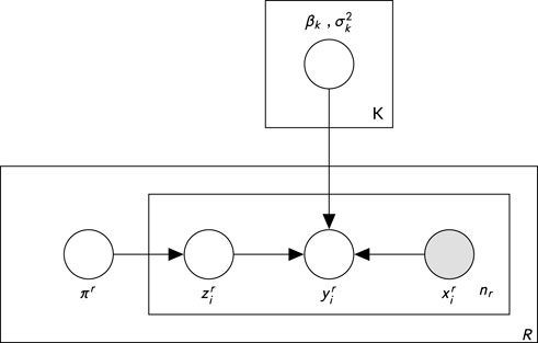
The model can also be represented as a probabilistic graphical model (Koller and Friedman, 2009), as shown in Figure 2. There are 2K + 1 “global” parameters ${\{{\beta }_k,{\sigma }_k^2\}}_{k=1}^K$ and π. Using the plate notation in this figure, there are R conditionally i.i.d. latent variables ${\{z^r\}}_{r=1}^R$ for each of the unique active regions. Under each active region r, there are n_r flare events ${\{(X_i^r,y_i^r)\}}_{i=1}^{n_r}$.

FIGURE 2

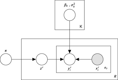
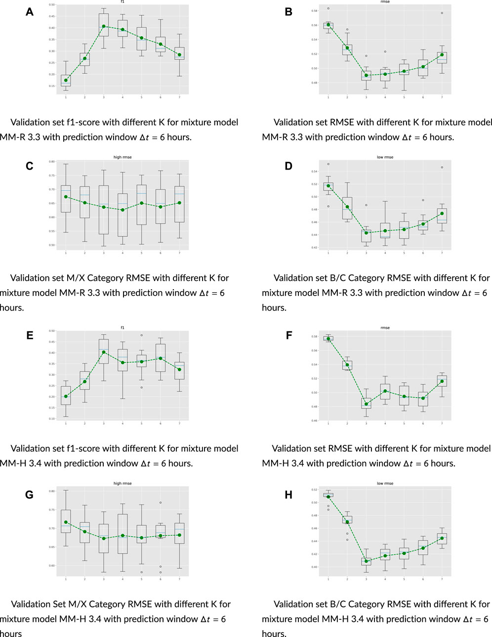
FIGURE 2. Model selection’s metrics for MM-R and MM-H. The x-axis is the number of mixture components to be selected.

Parameter estimation is achieved through an expectation-maximization algorithm (Dempster et al., 1977), with the lower bound as a weighted complete log-likelihood, as defined in section 3.2, and we optimize the weighted complete log-likelihood to remediate the data imbalance problem. Under this model, rather than the standard expected complete log-likelihood, our EM algorithm optimizes the weighted expected complete likelihood optimization problem,

$\begin{array}{ll}\hfill & {\text{argmax}}_{\pi ,{\sigma }^2,\beta }{\displaystyle \sum _{k=1}^K}{\displaystyle \sum _{r=1}^R}\mathbb{E}\left[z^r=k|X^r,y^r\right]\left[\log {\pi }_k-{\displaystyle \sum _{i=1}^{n_r}}\left(\frac{w_i}{2}\log {\sigma }_k^2\right.\right.\hfill \\ \hfill & \left.\left.+\frac{w_i}{2{\sigma }_k^2}\cdot {\left(y_i^r-{\beta }_k^T{X}_i^r\right)}^2\right)\right].\hfill \end{array}$

The E-step computes

${\tau }_k^r=p\left(z^r=k|X^r,y^r\right)=\frac{{\pi }_k\cdot \prod _{i=1}^{n_r}\text{N}\left(y_i^r|{\beta }_k^T{X}_i^r,{\sigma }_k^2\right)}{{\displaystyle \sum _{j=1}^K}{\pi }_j\cdot \prod _{i=1}^{n_r}\text{N}\left(y_i^r|{\beta }_j^T{X}_i^r,{\sigma }_j^2\right)}.$

The M-step yields

$\begin{array}{c}{\widehat{\pi }}_k=\frac{{\displaystyle \sum _{r=1}^R}{\tau }_k^r}{R},\\ {\widehat{\beta }}_k={\left[{\displaystyle \sum _{r=1}^R}{\tau }_k^r{\displaystyle \sum _{i=1}^{n_r}}{w}_i{X}_i^r{\left(X_i^r\right)}^T\right]}^{-1}\left[{\displaystyle \sum _{r=1}^R}{\tau }_k^r{\displaystyle \sum _{i=1}^{n_r}}{w}_i{y}_i^r{X}_i^r\right],\\ {\widehat{\sigma }}_k^2=\frac{{\displaystyle \sum _{r=1}^R}{\tau }_k^r{\displaystyle \sum _{i=1}^{n_r}}{w}_i\cdot {\left(y_i^r-{\widehat{\beta }}_k^T{X}_{i,r}\right)}^2}{{\displaystyle \sum _{r=1}^R}{n}_r\cdot {\tau }_k^r}.\end{array}$

Next, for prediction, on one hand, if the region of a new data point ${\tilde{X}}_i$ is not known, we estimate the log intensity ${\widehat{y}}_i|{\tilde{X}}_i={\sum }_{k=1}^K{\pi }_k\cdot {\tilde{X}}_i^T{\beta }_k$. On the other hand, if its region is r_i, then ${\widehat{y}}_i|r_i,{\tilde{X}}_i={\sum }_{k=1}^K{\tau }_{r_i,k}\cdot {\tilde{X}}_i^T{\beta }_k$.

3.4 Mixture model over flare events

The mixture model MM-R given in Section 3.3 requires all the flare events of an active region to follow the same regression pattern. This condition can be too restrictive. Note that in our dataset, each flare occurs at a different location and time within an active region, and we can think of the entire data being a collection of events from many active regions. Now, it is reasonable to accommodate the possibility that the heterogeneous nature extends further into each individual flare event within an active region. To model this behavior, we can assign a latent variable $z_i^r$ to each data point i but impose that $z_i^r\sim \text{Cat}(\cdot |{\pi }_i^r)$, where ${\pi }^r\in {\mathbb{R}}^K$ and ${\sum }_{k=1}^K{\pi }_k^r=1$. The parameter ${\pi }_k^r$ captures a regional inclination for certain categories of the flaring mechanism. If π^r(s) are extreme, e.g., taking value 1 in one coordinate and zeros elsewhere, the model MM-H is reduced to the mixture model MM-R given in the previous section. Note that this type of model is sometimes called a mixed membership model in the statistical learning literature (Airoldi et al., 2014), where an active region is a group of members, where the members, in this case, are its flare events. As discussed previously, the weighted complete log-likelihood is optimized to combat the unbalanced data.

Mathematically, the model is parameterized by ${\beta }_1,\dots ,{\beta }_K,{\sigma }_1^2,\dots ,{\sigma }_K^2,{\pi }^1,\dots ,{\pi }^R$, where K is the number of global parameters and R is the number of active regions. For active region r = 1, … , R,

$\begin{array}{ll}\hfill & z_i^r\sim \text{Cat}\left(\cdot |{\pi }^r\right),i=1,\dots ,n_r\hfill \\ \hfill & y_i^r|z_i^r=k,X_i^r\sim \text{N}\left(\cdot |{\beta }_k^T{X}_i^r,{\sigma }_k^2\right).\hfill \end{array}$

Figure 3 is the probabilistic graphical model representation of model MM-H. There are 2K “global” parameters ${\{{\beta }_k,{\sigma }_k^2\}}_{k=1}^K$. With the plate notation, there are now $n={\sum }_{r=1}^R{n}_r$ latent variables $z_i^r$ for each flare event $(X_i^r,y_i^r)$ of active region r. Under each active region r, the latent variable $z_i^r$ is a discrete random variable which takes values in {1, … , K} with probability weight π^r. Compared to the model described in Section 3.3, MM-R only has R latent variables z^r, with one “global” weight π. MM-H provides each active region the flexibility of having its own categorical weight π^r over K linear mechanisms.

FIGURE 3

FIGURE 3. MM-R and MM-H’s log intensity and estimated variance of each cluster.

Similar to the previously discussed model, the likelihood is $p(y_i^r|x_i^r;\pi ,\beta ,{\sigma }^2)={\sum }_{k=1}^K{\pi }_k^r\cdot N\left(\cdot |{\beta }_k^T{x}_i^r,{\sigma }_k^2\right)$, and the weighted expected complete log-likelihood optimization problem is equivalent to

$\begin{array}{ll}\hfill & {\text{argmax}}_{\beta ,\pi ,{\sigma }^2}{\displaystyle \sum _{k=1}^K}{\displaystyle \sum _{r=1}^R}{\displaystyle \sum _{i=1}^{n_r}}\mathbb{E}\left[z_i^r|y_i^r,X_i^r\right]\cdot \left(\log {\pi }_k^r-\frac{w_i}{2}\log {\sigma }_k^2\right.\hfill \\ \hfill & \left.-\frac{w_i}{2{\sigma }_k^2}\cdot {\left(y_i^r-{\beta }_k^T{X}_i^r\right)}^2\right).\hfill \end{array}$

Under these specifications, for parameter estimation, the iterative E-step computes

${\tau }_{i,k}^r=\mathbb{P}\left(z_i^r=k|y_i^r,X_i^r\right)=\frac{{\pi }_k^r\cdot N\left(y_i^r|{\beta }_k^T{X}_i^r,{\sigma }_k^2\right)}{{\displaystyle \sum _{j=1}^K}{\pi }_j^r\cdot N\left(y_i^r|{\beta }_j^T{X}_i^r,{\sigma }_j^2\right)},$

while the M-step performs the updates

$\begin{array}{ll}\hfill & {\widehat{\pi }}_k^r=\frac{{\displaystyle \sum _{i=1}^{n_r}}{\tau }_{i,k}^r}{n_r}\hfill \\ \hfill & {\widehat{\beta }}_k={\left[{\displaystyle \sum _{r=1}^R}{\displaystyle \sum _{i=1}^{n_r}}{\tau }_{i,k}^r\cdot w_i\cdot X_i^r{\left(X_i^r\right)}^T\right]}^{-1}\left[{\displaystyle \sum _{r=1}^R}{\displaystyle \sum _{i=1}^{n_r}}{\tau }_{i,k}^r\cdot y_i^r{X}_i^r\right]\hfill \\ \hfill & {\widehat{\sigma }}_k^2=\frac{{\displaystyle \sum _{r=1}^R}{\displaystyle \sum _{i=1}^{n_r}}{\tau }_{i,k}^r{w}_i\cdot {\left(y_i^r-{\widehat{\beta }}_k^T{X}_{i,r}\right)}^2}{{\displaystyle \sum _{r=1}^R}{\displaystyle \sum _{i=1}^{n_r}}{\tau }_{i,k}^r}.\hfill \end{array}$

Finally, to perform prediction for a new data point ${\tilde{X}}_i$ of the region r_i, given $r_i,\widetilde{X_i}$, we take ${\widehat{y}}_i≔{\sum }_{k=1}^K{\pi }_k^r\cdot {\beta }_k^T.\widetilde{X_i}$.

4 Model selection and data analysis discussion

The model selection for mixture models concerns the choice of K, the number of mixture components. In this section, we focus our investigation on the dataset with a prediction time window Δt = 6 h. Recall that with Δt = 6 h, each response y_i is matched with SHARP parameters X_i 6 h before in the data. Similar results can be obtained with other prediction time windows Δt = 12, 24, 36, 48 h. For general regression problems, a common evaluation metric for model performance is the root mean squared error (rmse) = $\sqrt{{\sum }_{i=1}^n{(y_i-X_i^T\widehat{\beta })}^2}$. However, this metric can be misleading if the primary concern is the predictive performance of M/X future events because the data are imbalanced, with M/X events being rare. To assess the proposed models in a more balanced fashion, we can first discretize each of the continuous-valued y_i into binary-valued ${\tilde{y}}_i\in \{\mathrm{0,1}\}$, where $\widetilde{y_i}=\mathbb{1}(y_i>-5)$, which then takes advantage of standard classifier metrics such as precision, recall, and f1 score (the harmonic mean of precision and recall) (Goutte et al., 2005). If a model attempts to improve the overall rmse performance by over-optimizing B/C events at the expense of M/X, the recall will be affected and lead to a low f1 score. The higher the f1 metrics (i.e., closer to 1), the better the performance. This approach also allows us to compare our models with other methods in the solar flare forecasting literature, which are mostly black box machine learning classifiers. We also recall that in Section 2, we split the original training set into a sub-training set and a validation set.

The validation set is utilized to determine the optimal number of components K) and the above discretization binary threshold. For the 6-h dataset, the threshold −5.0 yields the best f1 performance in the validation. Next, we explain in detail how to choose the best K.

4.1 Model selection

Note that when mixture component K = 1, both models given in Section 3.3 and Section 3.4 reduce to a weighted linear regression model. To perform model selection, the test set is fixed, and the original train set is randomly split into a sub-train set and a validation set for 100 repetitions. For each repetition, we train weighted linear regression (Section 3.1), MM-R (Section 3.3), and MM-H (Section 3.4) on the sub-training set and then apply them to the validation set to obtain the box plots given in Figure 4. In the figures, each box plot visualizes the minimum, first quartile, median, third quartile, and maximum of the collection of generated metrics over 100 repetitions. The averages are also depicted as green dots. The numbers in the x-axis are the number of mixture components to be selected. For MM-R, setting K = 3 yields the best f1 score. A similar conclusion for K can be observed from the breakdown of the rmse for B/C and M/X categories.

FIGURE 4

FIGURE 4. Selected subset of covariate X under each cluster of MM-R.

The B/C rmse is at the lowest for K = 3, 4, 5, and the M/X rmse is at the lowest for K = 3, 4, as shown in Figures 4C, D. Taking all observations into consideration, we pick K = 3 for MM-R. Following a similar reasoning, we pick K = 3 for MM-H. Note that we combine the rmse of M/X categories and B/C categories since the M/X represents strong flares and B/C represents weak flares. In addition, we are most interested in early warnings of strong flares.

4.2 Analysis of mixture model fittings

In this section, we demonstrate the clustering results of the mixture model MM-R discussed in Section 3.3 and MM-H discussed in Section 3.4 after training on the observed data. We inspect clustering effects on the marginal space of response y and the marginal space of covariate X, and then we explore what clustering structure entails the interactions between y and X.

4.2.1 Response space y

Examining the log intensities of each cluster provides hints on the interpretation of the clustering structures of the trained models. Specifically, by the above model selection procedure, we choose K = 3 for the mixture model MM-R. The red line in Figure 5A is the average of the response y over the entire training dataset. The median of cluster 1 is below the line. On the other hand, the median of cluster 2 is very close to it, and the median of cluster 3 is above it. This suggests that cluster 1 mostly consists of regions producing weak flares, and cluster 3 contains those with strong flares, while cluster 2 is in between. A similar conclusion is made regarding the mixture model over flare events MM-H with K = 3.

FIGURE 5

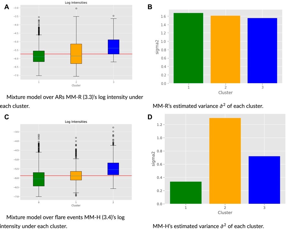
FIGURE 5. Mixture model over ARs estimated $\{{\widehat{\beta }}_1^K\}$ and each active region’s mixing proportions of these values.

4.2.2 Covariate space X

The same clustering interpretation can be extracted by inspecting covariate values for each cluster given in Figures 6A–F. It has been scientifically observed that the flare intensities are connected to the magnetic properties of the active region. Using model MM-R, by inspecting the relevant magnetic covariate features, we found that cluster 1 has lower numeric values under both weak (B/C) and strong (M/X) events than the others. In contrast, cluster 3 has the highest values. This further corroborates the interpretation that cluster 1 mainly has weak flare events, cluster 3 is populated with strong events, and cluster 2 is in between. Similarly, we can reach the same conclusion for the model over flare events, MM-H; the corresponding plots are provided in Figure 17.

FIGURE 6

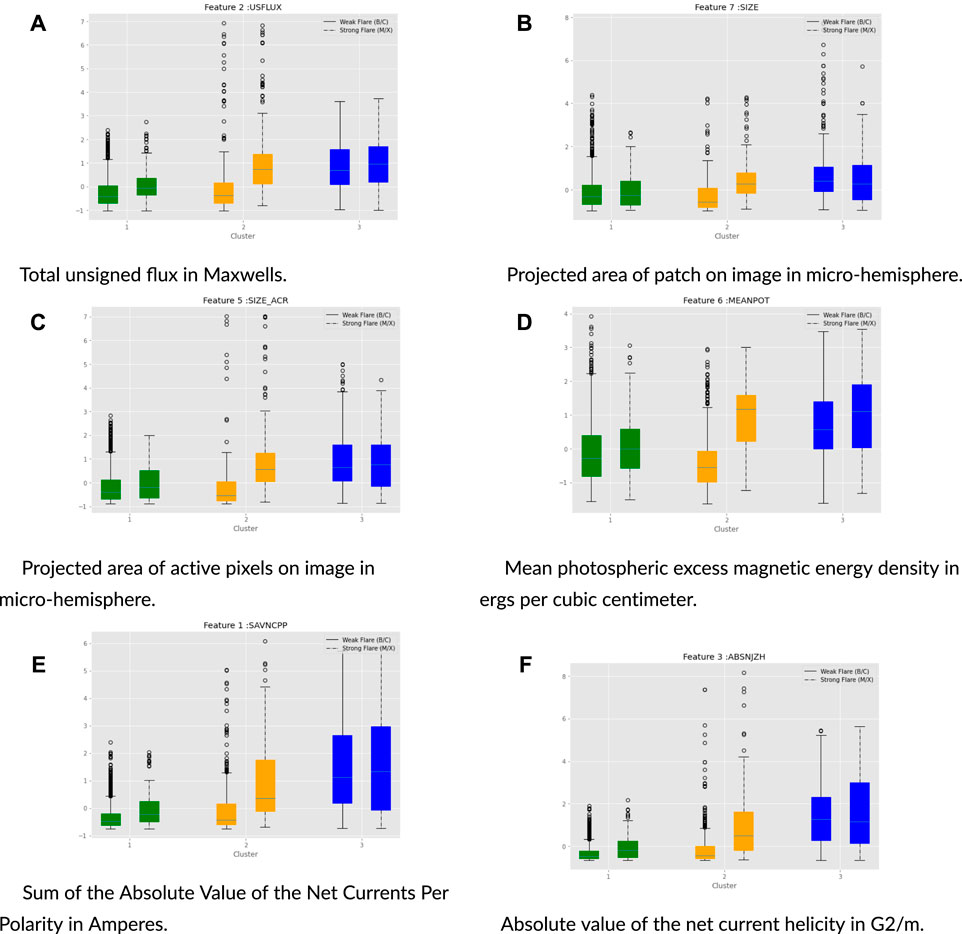
FIGURE 6. Active Region 11967’s SHARP parameters and HMI image during its strongest flare event and bar plots of regression coefficients on the right. AR 11967 existed from 2014/01/30 to 2014/02/08. The dash lines are the times at their peak intensities. The solid lines are the 6-hour-before for covariates’ regression.

4.2.3 Interaction between the covariate X and response y

Under the standard multivariate linear regression setting, the coefficient $\beta \in {\mathbb{R}}^d$ indicates how much the response y is expected to increase when an independent variable increases by one unit, holding all other independent variables constant. For heterogeneous regression responses, the interaction between covariates X and y is, to a certain extent, more delicate. In particular, for MM-R, three global coefficient parameters exist: β₁, β₂, β₃. Now, how do we interpret them and talk about the interaction between y and X?

Recall that under MM-R, the predicted $\widehat{y}$ for flare event i in AR r is given by

$\begin{array}{l}\hfill \begin{array}{cc}\hfill {\widehat{y}}_i^r& ={\displaystyle \sum _{k=1}^K}{\tau }_k^r{\beta }_k^T{X}_i^r={\left[{\displaystyle \sum _{k=1}^K}{\tau }_k^r{\beta }_k\right]}^T\cdot X_i^r\hfill \\ \hfill & ={\left[{\displaystyle \sum _{k=1}^K}p(z^r=k|X_1^r,\dots ,X_{n_r}^r,y_1^r,\dots ,y_{n_r}^r){\beta }_k\right]}^T\cdot X_i^r≕{({\beta }^r)}^T{X}_i^r.\hfill \end{array}\end{array}$

Thus, under active region r, β^r indicates how much the response $y_i^r$ is expected to increase by increasing an independent variable by one unit, holding other variables fixed. Furthermore, ${\{{\tau }_k^r\}}_1^K$ controls the influence of each β_k on β^r, the interaction coefficient between y and X for region r. If we visualize β₁, β₂, and β₃ as three extreme points, e₁, e₂, e₃ = (0, 0; 1, 0; 0, 1) in a 2D unit simplex, and plot each AR r at the coordinate ${\tilde{c}}^r≔{\sum }_{k=1}^3{\tau }_k^r{e}_k$ (note that all flare events i under AR r have the same β^r), then, the position of AR r in the simplex indicates visually how much it is influenced by each of the global ${\{{\beta }_k\}}_{k=1}^3$. Furthermore, we can inspect the mixture component assignments for all active regions under the trained model MM-R as illustrated in Figure 7. Figure 7B shows the coefficient β^r of each AR r under the influence of clusters 1 (green), 2 (yellow), and 3 (blue). Each AR is visualized as a colored dot in the unit simplex, and its size corresponds to the number of flare events recorded in that AR. In Figure 7B, we observe that active regions under cluster 1 (green) are mainly affected by ${\widehat{\beta }}_1$, but ${\widehat{\beta }}_2$ still plays some role, while ${\widehat{\beta }}_3$ has a negligible impact. By the same manner of reasoning, cluster 2 (yellow) is mainly influenced by ${\widehat{\beta }}_2$, and ${\widehat{\beta }}_1$ plays a relatively minor role. Cluster 3 (blue) is mostly affected by parameters ${\widehat{\beta }}_3$. Figure 7A shows the magnitudes of each feature for ${\widehat{\beta }}_1,{\widehat{\beta }}_2$ and ${\widehat{\beta }}_3$. Each has 17 bars. The first bar is the linear regression intercept coefficient, and the following bars are the coefficients of features: TOTUSJH, SAVNCPP, USFLUX, ABSNJZH, TOTPOT, SIZE_ACR, MEANPOT, SIZE, MEANJZH, SHRGT45, MEANJZD, MEANALP, MEANGBT, MEANGAM, MEANGBZ, and MEANGBH. Their descriptions are given in Table 2. The same line of interpretation can be applied for MM-H, for which similar plots are included in Figures 8A, B of the appendix.

FIGURE 7

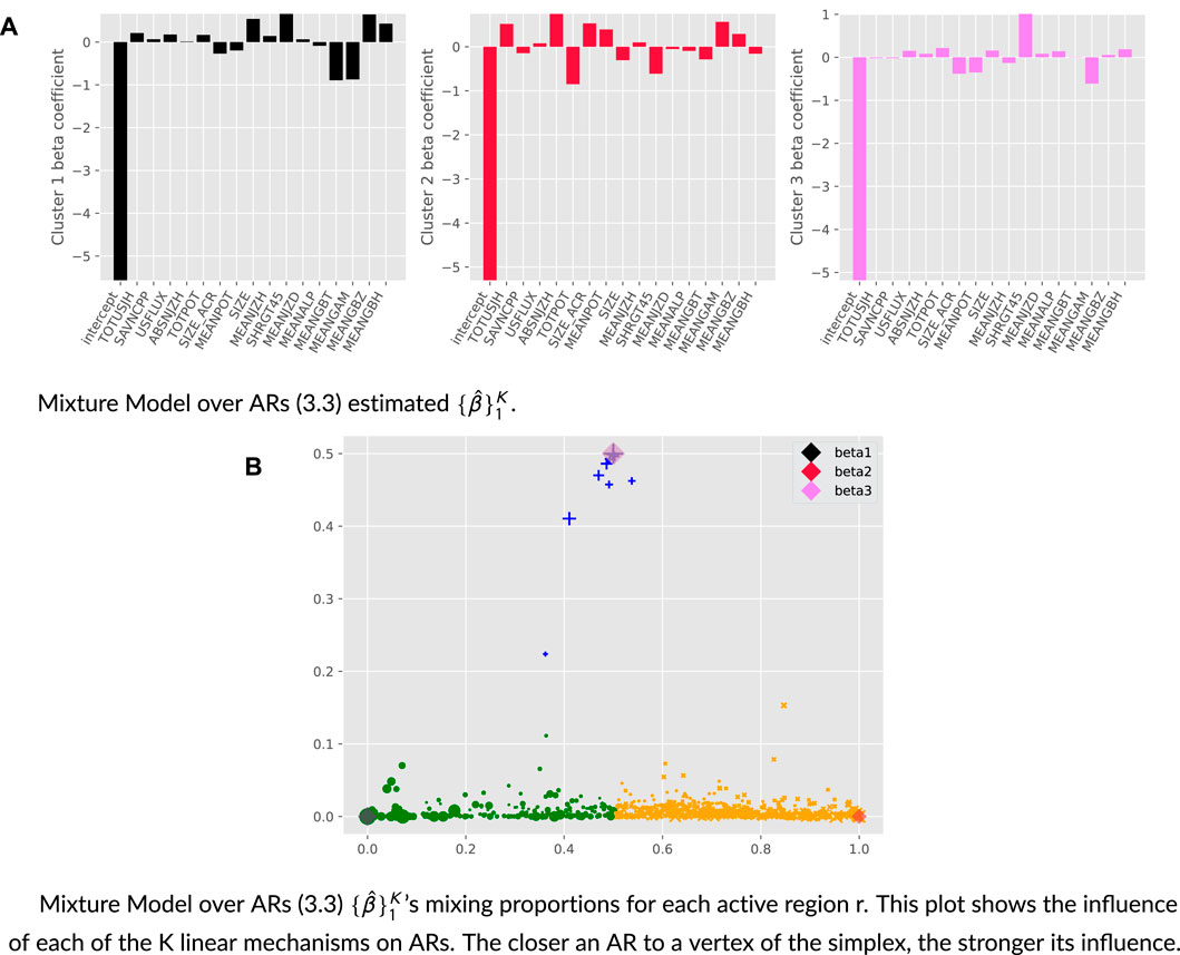
FIGURE 7. The left two images are radial components and right two ones are horizontal filed in AR 12242 (H label) at its strongest (2014.12.20_00:28:00) and weakest flare events (2014.12.16_00:05:00) during its existence. AR 12242 existed from 2014/12/14 to 2014/12/21.

FIGURE 8

FIGURE 8. Active Region 12242’s SHARP parameters. AR 12242 existed from 2014/12/14 to 2014/12/21.

4.3 Prediction performance

Note again that when the number of mixture components K = 1, the models discussed in Section 3.3 and Section 3.4 are just the weighted linear regression model. To produce the figures given in Tables 3–6, we train standard linear regression, weighted linear regression, and models MM-R (Section 3.3) and MM-H (Section 3.4) on the training data, as described in the data section. We run MM-R and MM-H for 100 replications, under each of which training and testing datasets are randomly split, as described in Section 2. We then take the averages as the final results. For each replication, we run our EM procedures five times and select the one with the highest likelihood as the fitted model. We use the validation set to pick the best number of components K. Even though the models predict continuous responses, and we can assess their rmse, to help illustrate the model performances against data imbalance, of which the rmse is not particularly helpful, we compute the f1 score. Since this is a classification metric, continuous responses need to be converted into binary outcomes. We use the same validation set to pick the best binary splitting thresholds. The estimated binary responses are compared with the true labels of strong flares (M/X) and weak flares (B/C) in the data.

TABLE 3

TABLE 3. (Unweighted) linear regression test performance.

TABLE 4

TABLE 4. Weighted linear regression test performance.

TABLE 5

TABLE 5. Test performance of the mixture model over ARs. Note: the f1 score is computed based on K =3,3,3,3,5, and classification threshold = −5.0,−5.0,−5.05,−5.1,−5.15.

TABLE 6

TABLE 6. Test performance of the mixture model over flare event. Note: the f1 score is computed based on K =3, 3, 3, 6, 5, and classification threshold = −5.0,−5.0, −5.05, −5.05, −5.1.

The numbers given in Tables 3–6 show that mixture models MM-H (Section 3.4) and MM-R perform similarly, although the former is marginally better. MM-R and MM-H (Section 3.4) significantly outperform the weighted linear regression. This result implies that adding more components improves the performance and, thus, supports the heterogeneous nature of the data. Model MM-H offers more flexibility by extending the heterogeneity pattern to individual flare events. However, interestingly, this flexibility does not noticeably improve the defined metrics. This suggests that the heterogeneity signal is most noticeable at the active region level. We also observe that the performance degrades as the predicting time windows increase, which is expected. Finally, we remark that our predictive performance in the f1 metric (0.383) for 6-h data is lower than that observed by Chen et al. (2019). This is not surprising as we assume linear relationships between covariates and responses and do not account for the temporal nature of solar flares, where future events may correlate with past events. In contrast, Chen et al. (2019) constructed a sophisticated LSTM neural network to extract complex nonlinear signals from the data. We describe potential future directions for improving model performance in the last section. However, the main contribution of this work is demonstrating how mixture models can cluster solar active regions based on the interaction mechanisms between their SHARP covariates and corresponding intensity responses, thus characterizing the heterogeneous nature of active regions.

4.4 Case studies

Both models MM-R 3.3 and MM-H 3.4 perform similarly regarding f1 metrics, even though MM-H is marginally better. As mentioned in the last section, this result seems to suggest that flares from the same AR are intrinsically homogeneous in nature or homologous, as known to the solar physics community (Manchester, 2003; Sui et al., 2004; Liu et al., 2014; Romano et al., 2018). In contrast, individual ARs are most often heterogeneous. As such, we use MM-R for the case studies in this section. As stated in the introduction, the goal of this project is to characterize the heterogeneity among ARs. The cluster membership of the fitted models is particularly interesting, because the model MM-R groups similar active regions together in each cluster.

Because the training and testing sets are created randomly, mixture memberships might change in different replications of the model fitting procedure. Thus, to analyze the cluster assignment in a robust manner, we run the model fitting procedure for MM-R for 100 repetitions. In each repetition, active regions are allocated to different mixture clusters. To standardize the meaning of clusters across repetitions, we assign labels “H,” “L,” and “I” to mixture clusters of which the first quartile of its collections of log intensities is greater than −5.75, smaller than −6.0, and between [−6, −5.75], respectively. By the design of the log intensity threshold for “H,” “I,” and “L,” active regions allocated to “H” labels should be reasonably active in terms of strong flare events, active regions to allocated “L” should be relatively quiet, and “I” in between.

We observe that some active regions have the same labels for all 100 repetitions. For example, ARs 11,124 and 11,109 are assigned to the label “L” in each of the 100 iterations. On the other hand, other active regions might be allocated to different labels over 100 repetitions. For instance, AR 11,967 is assigned to cluster “H” 87% and “I” 13% of the 100 repetitions or AR 12192 85% “H” and 15% “I.” The reason why an active region may have different labels for different repetitions has to do with the randomness of data splitting. In particular, AR 11153 has 28 flare events, of which only one is M class and the rest are B and C ones. As such, if the M-class event is included in the training, it will skew the average log intensities higher than otherwise, and so, it affects its mixture cluster assignment.

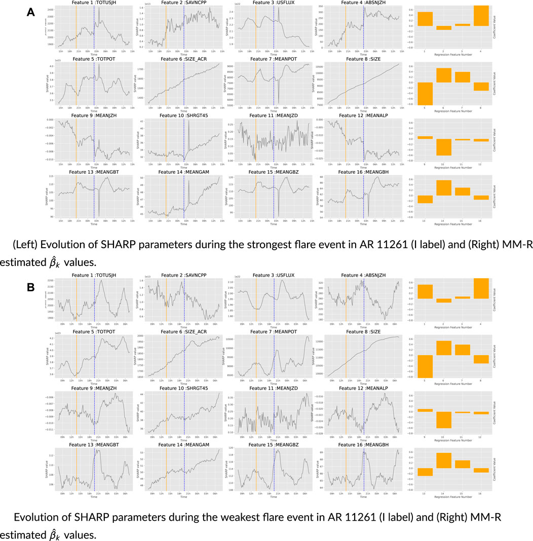
The complete list of active region membership is provided in Supplementary Material. Here, we mention the top two ARs for each of the labels “H,” “I,” and “L” in terms of the highest number of label assignments in 100 repetitions. Regarding the “L” label, ARs 11,117 and 11,109 are assigned to “L” 99% and 100% of the times, respectively. For “H,” ARs 11,967 and 12,242 are assigned to “H” 87% and 88% of the times, respectively. For “I,” ARs 11,261 and 11,087 are allocated to “I” 62% and 59% of the 100 repetitions, respectively. Some existing works in the space weather literature corroborate that ARs 11,967 and 12,242 were known to produce strong flares (Solovev et al., 2019; Durán et al., 2020; Joshi et al., 2021). A common trait of ARs with the “I” label is that they have few strong flares among a majority of quiet flare events. In contrast, ARs with “L” labels have only quiet flare events.

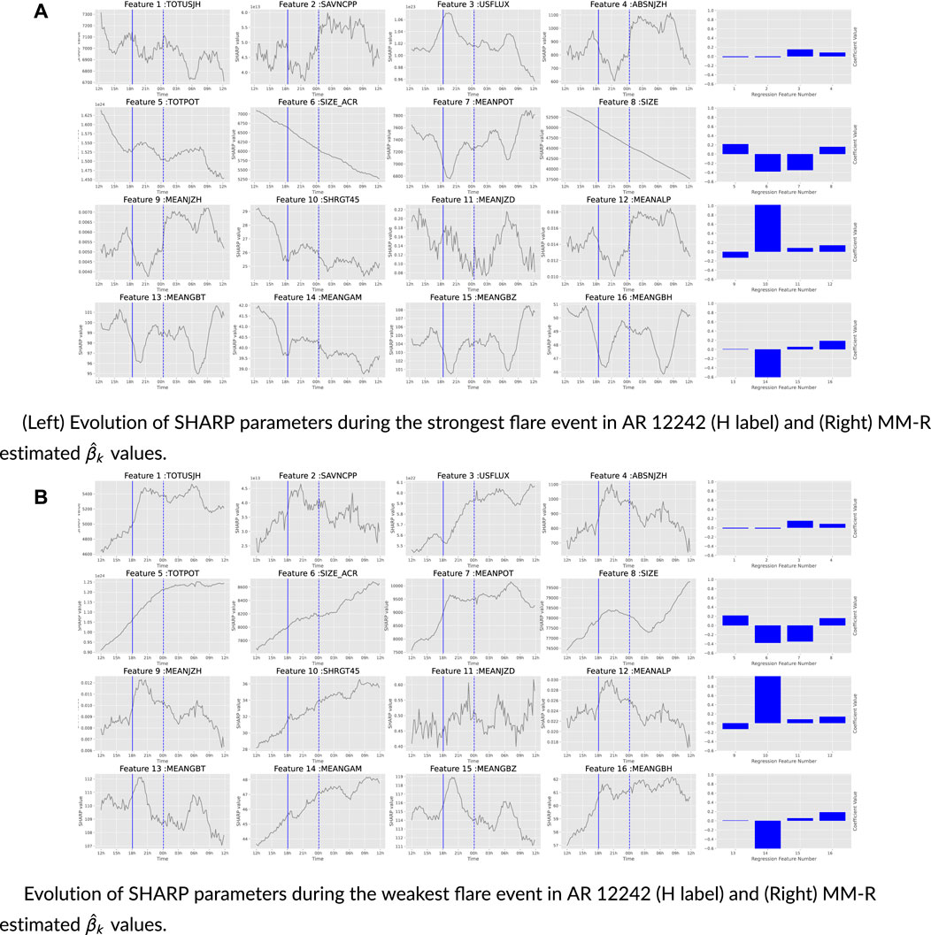
To complete our case study, we provide the HMI image and the temporal evolution of each SHARP parameter for the strongest and weakest flare events for AR 11,967 during its existence from January 27 2014 to February 09 2014 in Figure 16. Appendix B provides the same plots for all ARs 11,117, 11,261, 11,967, and 12,242.

FIGURE 10

FIGURE 10. Active Region 11261’s SHARP parameters. AR 11261 existed from 2011/7/28 to 2011/8/5.

FIGURE 11

FIGURE 11. Active Region 11117’s SHARP parameters. AR 11117 existed from 2010/10/21 to 2010/10/31.

FIGURE 12

FIGURE 12. MM-H’s estimated $\{{\widehat{\beta }}_1^K\}$ and the mixing proportion w.r.t these $\widehat{\beta }$ for each flare event.

FIGURE 13

FIGURE 13. Selected subset of covariate X under each cluster of MM-H.

FIGURE 14

FIGURE 14. The left two images are radial components, and the right two images are horizontal, filed in AR 11,117 (L label) at its strongest (2010.10.31_04:31:00) and weakest (2010.10.22_07:59:00) flare events during its existence. AR 11,117 existed from 2010/10/21 to 2010/10/31.

FIGURE 16

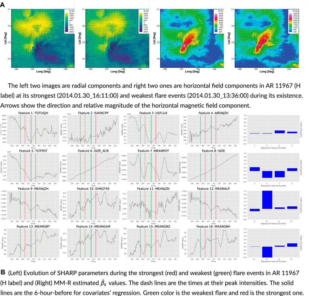
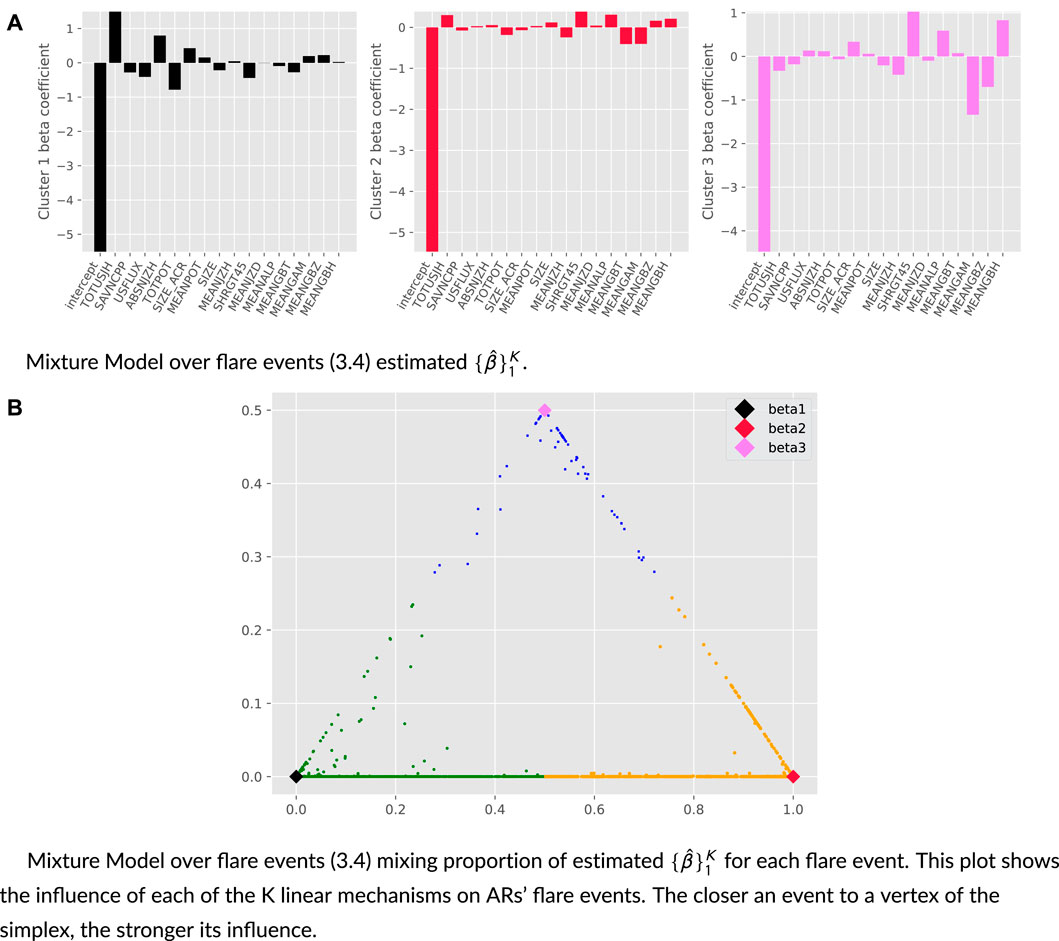
FIGURE 16. SHARP parameters and HMI image of active region 11,967 during its strongest flare event. The bar plots of regression coefficients are on the right. AR 11967 existed from 2014/01/30 to 2014/02/08. The dashed lines are the times at their peak intensities. The solid lines are the 6-hour-before for covariates’ regression. (A) Mixture model over flare events estimated {βˆ}^K₁. (B) Mixture model over flare events mixing proportion of estimated {βˆ}^K₁ for each flare event. This plot shows the influence of each of the K-linear mechanisms of the flare events on ARs. The closer an event is to a vertex of the simplex, the stronger its influence.

FIGURE 17

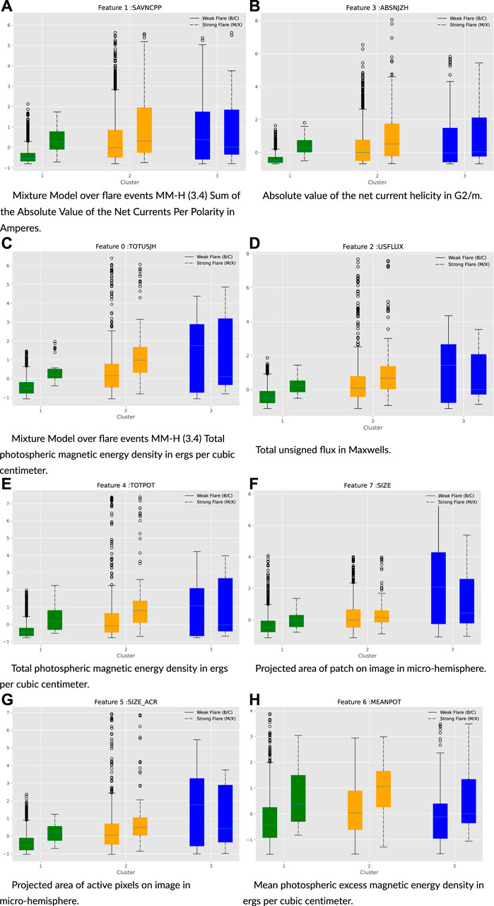
FIGURE 17. Selected subset of covariate X under each cluster of MM-H. (A) Mixture Model over flare events MM-H (3.4) sum of the absolute value of the net currents per polarity in amperes. (B) Absolute value of the net current helicity in G2/m. (C) Total photospheric magnetic energy density in ergs per cubic centimeter of MM-H. (D) Total unsigned flux in maxwells. (E) Total photospheric magnetic energy density in ergs per cubic cm. (F) Projected area of patch on image in micro-hemisphere. (G) Projected area of active pixels on image in micro-hemisphere. (H) Mean photospheric excess magnetic energy density in ergs per cubic cm.

a) The left two images are radial components, and the right two ones are horizontal field components in AR 11967 (H label) at its strongest (2014.01.30_16:11:00) and weakest (2014.01.30_13:36:00) flare events during its existence. Arrows show the direction and relative magnitude of the horizontal magnetic field component.

b) (Left) Evolution of SHARP parameters during the strongest (red) and weakest (green) flare events in AR 11967 (H label) and (Right) MM-R estimated ${\widehat{\beta }}_k$ values. The dashed lines are the times at their peak intensities. The solid lines are the 6-hour-before for covariates’ regression. The green color is the weakest flare, and red is the strongest one.

All flaring active regions share common basic features, which is a nonpotential magnetic field forming a filament channel over a well-defined polarity inversion line (Green et al., 2018). Beyond this basic feature, there are many possible avenues to eruption. Here, we summarize the observed magnetic structure and evolution of cluster members to determine whether there are features or processes responsible for the heterogeneity of the mixture models. The H cluster contains numerous X-class flares, which received considerable attention in the published literature. The conditions of AR 12,242 leading to the X1.8 flare on December 20 2014 are particularly well described. For example, Solovev et al. (2019) describes the convergence of magnetic flux toward the polarity inversion line leading to both a local and a total maximum gradient of the magnetic field at the time of the flare. Solovev et al. (2019) further described the formation of a magnetic flux rope by reconnection between the converging/colliding sunspots, which erupts to produce the flare. This flaring process has been developed by numerous authors, e.g., Chintzoglou et al. (2019) and Liu (2020). In the case of AR 11,967, a series of flares occurred at a sunspot light bridge, a region of extremely intense and highly sheared magnetic fields produced by flux emergence (Kawabata et al., 2017; Durán et al., 2020). In both examples, we find an intensification of the magnetic field.

For the I cluster, we again find well-described events showing consistent patterns of evolution leading to the flares. The strongest flare from AR 11,087, a C2.7 event, occurred on July 13 2010 at 10:51:00 UT, which is described by Joshi et al. (2015). The flare is characterized by the activation and partial eruption of an active region filament that produces a pair of flair ribbons. Another member of the I cluster, AR 11,261, produced a series of flares, including 4 M-class events, which arose from a complex system of 4 sunspots, one being in a delta configuration (Thalmann et al., 2016). Ye et al. (2018) found that shearing of the photospheric magnetic field associated with flux emergence was a key driver of flares. These observations are consistent with Lorentz force-driven shear flows powering solar eruptions (Ward, 2001; Manchester, 2003; Manchester et al., 2004; Ward, 2007; Fang et al., 2010). Similarly, Sarkar et al. (2019) found that the free energy necessary for flares from active region 11,261 was provided by the shearing motion of moving magnetic features of opposite polarities near the polarity inversion line. The authors also found patterns in the time evolution of the net Lorentz force associated with solar flares.

As stated earlier, the L cluster is dominated by weak flares, which poses two challenges. First, the events are so low in energy that they often occur without significant changes in the photospheric magnetic field and without clear precursors. Second, these low-energy events are far less documented in the literature. However, active region 11,117 is an exception being described in detail in a series of papers by Jiang et al. (2012); Jiang et al. (2016); and Jiang et al. (2017), which we recount here. This region produced a series of small B-class flares observed on October 25 2010 (a date in between our strong and weak flare events), culminating in a C2.3-class event. As described by Jiang et al. (2012), the coronal loops of active region 11,117 (observed by AIA-171) remained largely unchanged, but a flare reconnection was observed at the location of a magnetic null derived from their nonlinear force-free field (NLFFF) model. This eruption event is consistent with topologically driven reconnection models (Titov et al., 2010; Liu et al., 2016). In this case, observations show shear and rotational motions at the photosphere, providing a clear buildup of energy preceding the flares, but no sudden changes precipitate a flare.

5 Conclusion and future work

In this paper, our goal is the characterization of the heterogeneous patterns shared by different active regions on the surface of the Sun based on data-driven approaches. We propose two types of mixture models: MM-R and MM-H. The first model, MM-R, is designed to specify the heterogeneity across active regions. The second model, MM-H, goes beyond to specify the heterogeneity for flaring patterns within an active region. As demonstrated, using mixture modeling improves the performance of the solar flare prediction. The second model, MM-H, performs marginally better. Since the extension of heterogeneity to individual flare events within an active region, as explained in Section 3.4, does not yield conclusive gains, the heterogeneous nature of the mixture seems to be strongly due to active regions, while flaring events within active regions tend to be more homogeneous. Another contribution of this paper is showing how to deal with the imbalance problem using the expectation-maximization framework.

Significantly, our work demonstrates the clustering results of the mixture model MM-R. We observed three clusters, namely, “H,” “I,” and “L.” As our mixture model is designed to perform clustering at the level of interaction between covariates and responses, it implies three distinct linear mechanisms for three clusters. Moreover, the “H” group of ARs produces significantly more strong flares, while ARs in group “I” have few strong flares and a majority of weak flare events. In contrast, ARs with “L” labels have only weak flare events.

An equally important result is based on the fact that MM-H is marginally better than MM-R, which demonstrates that flares from the same AR are intrinsically homogeneous. This result is fully consistent with what was already known about homologous flares: the magnetic configuration remains similar between successive flares and is reformed between flare events. Such flares are readily explained by the reconnection of coronal magnetic fields, resulting in flare ribbons in the chromosphere (Sui et al., 2004; Liu et al., 2014; Janvier et al., 2023), which is now considered the standard model in solar physics. The energized field is in the form of a sheared core or filament channel, which persists or reforms by shearing motions after subsequent flares (Manchester, 2003; Romano et al., 2018).

The mixture model also discerns heterogeneity between active regions in three distinct clusters. The H cluster is representative of the most energetic events. These flares follow the sudden intensification of magnetic fields and their gradients, which can follow from the emergence of intense magnetic fields or large-scale collisions of opposite polarities. This evolution comes with clear and distinct signatures of the covariates. The I-class events follow a buildup of energy from shear and rotational flows associated with lower levels of emerging magnetic fields. At lower energies, a buildup of energy eventually activates flares from a topological feature. The I and L classes show more similarity with shear and rotational flows producing an energy buildup. However, while the I class is associated with flux emergence, the least energetic L-class events follow an energy buildup, with little emergence occurring over the time scale of the flare events. In this sense, a clear pattern is related to the relative disruption of the photospheric magnetic field driving the flare events.

In this work, we assume an independent linear relationship between X_i and y_i for each data point in a mixture cluster. This does not take into account the fact that flares occur through time, and there may be a temporal correlation between a future event and past events. The next step is to adopt more sophisticated regression methods, such as Gaussian process regression. Moreover, we can also apply a more powerful approach to determine the number of mixture components. Existing methodologies like the Dirichlet process or hierarchical Dirichlet process seem to be a promising direction to pursue.

6 EM algorithm derivation

For mixture model MM-R defined in Section 3.3, we can write the complete likelihood as

$\begin{array}{ll}\hfill & p\left.\left(y_1,y_2,\dots y_n,z^1,\dots ,z^R|X_1,X_2,\dots ,X_n\right)\right)\hfill \\ \hfill & =\prod _{r=1}^{R}p\left(z^r\right)\prod _{i=1}^{n_r}p\left(y_i^r|z^r,X_i^r\right)\hfill \\ \hfill & =\prod _{r=1}^R\prod _{k=1}^K{\left[{\pi }_k\prod _{i=1}^{n_r}p\left(y_i^r|z^r=k,X_i^r\right)\right]}^{\mathbb{1}\left(z^r=k\right)}.\hfill \end{array}$

So, the complete log-likelihood can be written as

$\begin{array}{ll}\hfill l\left(\beta ,z\right)& =\left.\log p\left(y_1,y_2,\dots y_n,z^1,\dots ,z^R|X_1,X_2,\dots ,X_n\right)\right)\hfill \\ \hfill & ={\displaystyle \sum _{r=1}^R}{\displaystyle \sum _{k=1}^K}\mathbb{1}\left(z^r=k\right)\cdot \left[\log {\pi }_k+{\displaystyle \sum _{i=1}^{n_r}}\log p\left(y_i^r|z_i^r=k,X_i^r\right)\right].\hfill \end{array}$

Since $y_i^r|X_i^r,z_i^r=k\sim \text{N}(\cdot |{\beta }_k^T{X}_i^r,{\sigma }_k^2)$, by denoting ${\tau }_k^r≔\mathbb{E}[z^r=k|X^r,y^r]$, the expected complete log-likelihood is

$\begin{array}{ll}\hfill el\left(\beta ,z\right)& ={\displaystyle \sum _{k=1}^K}{\displaystyle \sum _{r=1}^R}\mathbb{E}\left[z^r=k|X^r,y^r\right]\cdot \left[\log {\pi }_k-{\displaystyle \sum _{i=1}^{n_r}}\left(\frac{1}{2}\log {\sigma }_k^2\right.\right.\hfill \\ \hfill & \left.\left.-\frac{1}{2{\sigma }_k^2}\cdot {\left(y_i^r-{\beta }_k^T{X}_i^r\right)}^2\right)\right]\hfill \\ \hfill & ={\displaystyle \sum _{k=1}^K}{\displaystyle \sum _{r=1}^R}{\tau }_k^r\cdot \left[\log {\pi }_k-{\displaystyle \sum _{i=1}^{n_r}}\left(\frac{1}{2}\log {\sigma }_k^2\right.\right.\hfill \\ \hfill & \left.\left.-\frac{1}{2{\sigma }_k^2}\cdot {\left(y_i^r-{\beta }_k^T{X}_i^r\right)}^2\right)\right].\hfill \end{array}$

Now, as explained in previous sections, to combat the data imbalance issue, we optimize a weighted version of the complete log-likelihood:

$\begin{array}{ll}\hfill & {\text{arg\hspace{0.17em}max}}_{\beta ,\pi ,{\sigma }^2}{\displaystyle \sum _{k=1}^K}{\displaystyle \sum _{r=1}^R}{\tau }_k^r\cdot \left[\log {\pi }_k-{\displaystyle \sum _{i=1}^{n_r}}\left(\frac{w_i}{2}\log {\sigma }_k^2-\frac{w_i}{2{\sigma }_k^2}\right.\right.\hfill \\ \hfill & \left.\left.\cdot {\left(y_i^r-{\beta }_k^T{X}_i^r\right)}^2\right)\right].\hfill \end{array}$

For the M-step, taking derivatives w.r.t each parameter and setting to zeros, it can be seen that

$\begin{array}{ll}\hfill & {\widehat{\pi }}_k=\frac{{\displaystyle \sum _{r=1}^R}{\tau }_k^r}{R}\hfill \\ \hfill & {\widehat{\beta }}_k={\left[{\displaystyle \sum _{r=1}^R}{\tau }_k^r{\displaystyle \sum _{i=1}^{n_r}}{w}_i{X}_i^r{\left(X_i^r\right)}^T\right]}^{-1}\left[{\displaystyle \sum _{r=1}^R}{\tau }_k^r{\displaystyle \sum _{i=1}^{n_r}}{w}_i{y}_i^r{X}_i^r\right]\hfill \\ \hfill & {\widehat{\sigma }}_k^2=\frac{{\displaystyle \sum _{r=1}^R}{\tau }_k^r{\displaystyle \sum _{i=1}^{n_r}}{w}_i\cdot {\left(y_i^r-{\widehat{\beta }}_k^T{X}_i^r\right)}^2}{{\displaystyle \sum _{r=1}^R}{n}_r\cdot {\tau }_k^r}.\hfill \end{array}$

For the E-step,

$\begin{array}{ll}\hfill {\tau }_k^r& =\mathbb{E}\left(z^r=k|X^r,y^r\right)\hfill \\ \hfill & =\frac{{\pi }_{k}p\left(y^r|X^r,z^r=k\right)}{{\displaystyle \sum _{j=1}^K}{\pi }_{j}p\left(y^r|X^r,z^r=j\right)}\hfill \\ \hfill & =\frac{{\pi }_k\prod _{i=1}^{n_r}p\left(y_i^r|X_i^r,z^r=k\right)}{{\displaystyle \sum _{j=1}^K}{\pi }_j\prod _{i=1}^{n_r}p\left(y_i^r|X_i^r,z^r=j\right)}\hfill \\ \hfill & =\frac{{\pi }_k\cdot \prod _{i=1}^{n_r}\text{N}\left(y_i^r|{\beta }_k^T{X}_i^r,{\sigma }_k^2\right)}{{\displaystyle \sum _{j=1}^K}{\pi }_j\cdot \prod _{i=1}^{n_r}\text{N}\left(y_i^r|{\beta }_j^T{X}_i^r,{\sigma }_j^2\right)}.\hfill \end{array}$

Similarly, with model MM-H defined in Section 3.3, the expected complete log-likelihood is

$\begin{array}{ll}\hfill el\left(\beta ,z\right)& ={\displaystyle \sum _{k=1}^K}{\displaystyle \sum _{r=1}^R}{\displaystyle \sum _{i=1}^{n_r}}{\tau }_{i,k}^r\cdot \left[\log {\pi }_k^r-\left(\frac{1}{2}\log {\sigma }_k^2\right.\right.\hfill \\ \hfill & \left.\left.-\frac{1}{2{\sigma }_k^2}\cdot {\left(y_i^r-{\beta }_k^T{X}_i^r\right)}^2\right)\right],\hfill \end{array}$

where ${\tau }_{i,k}^r=\mathbb{E}(z_i^r=k|y_i^r,X_i^r)$. Again, to deal with the data imbalance, we work with the weighted optimization instead:

$\begin{array}{ll}\hfill & {\text{arg\hspace{0.17em}max}}_{\beta ,\pi ,{\sigma }^2}{\displaystyle \sum _{k=1}^K}{\displaystyle \sum _{r=1}^R}{\displaystyle \sum _{i=1}^{n_r}}{\tau }_{i,k}^r\cdot \left(\log {\pi }_k^r-\frac{w_i}{2}\log {\sigma }_k^2\right.\hfill \\ \hfill & \left.-\frac{w_i}{2{\sigma }_k^2}\cdot {\left(y_i^r-{\beta }_k^T{X}_i^r\right)}^2\right).\hfill \end{array}$

For the M-step, it is easy to derive

$\begin{array}{ll}\hfill & {\widehat{\pi }}_k^r=\frac{{\displaystyle \sum _{i=1}^{n_r}}{\tau }_{i,k}^r}{n_r}\hfill \\ \hfill & {\widehat{\beta }}_k={\left[{\displaystyle \sum _{r=1}^R}{\displaystyle \sum _{i=1}^{n_r}}{\tau }_{i,k}^r\cdot w_i\cdot X_i^r{\left(X_i^r\right)}^T\right]}^{-1}\left[{\displaystyle \sum _{r=1}^R}{\displaystyle \sum _{i=1}^{n_r}}{\tau }_{i,k}^r\cdot y_i^r{X}_i^r\right]\hfill \\ \hfill & {\widehat{\sigma }}_k^2=\frac{{\displaystyle \sum _{r=1}^R}{\displaystyle \sum _{i=1}^{n_r}}{\tau }_{i,k}^r{w}_i\cdot {\left(y_i^r-{\widehat{\beta }}_k^T{X}_{i,r}\right)}^2}{{\displaystyle \sum _{r=1}^R}{\displaystyle \sum _{i=1}^{n_r}}{\tau }_{i,k}^r}.\hfill \end{array}$

For the E-step,

$\begin{array}{ll}\hfill {\tau }_{i,k}^r& =\mathbb{E}\left(z_i^r=k|X_i^r,y_i^r\right)\hfill \\ \hfill & =\frac{{\pi }_k^{r}p\left(y_i^r|X_i^r,z_i^r=k\right)}{{\displaystyle \sum _{j=1}^K}{\pi }_{j}p\left(y_i^r|X_i^r,z_i^r=j\right)}\hfill \\ \hfill & =\frac{{\pi }_k\cdot \text{N}\left(y_i^r|{\beta }_k^T{X}_i^r,{\sigma }_k^2\right)}{{\displaystyle \sum _{j=1}^K}{\pi }_j\cdot \text{N}\left(y_i^r|{\beta }_j^T{X}_i^r,{\sigma }_j^2\right)}.\hfill \end{array}$

7 Case study plot and additional plots

Figures 9–15 display the radial components and horizontal field, along with the evolution of SHARP parameters, during the strongest and weakest flare events observed under AR 11967, 12242, 11261, and 11117.

FIGURE 9

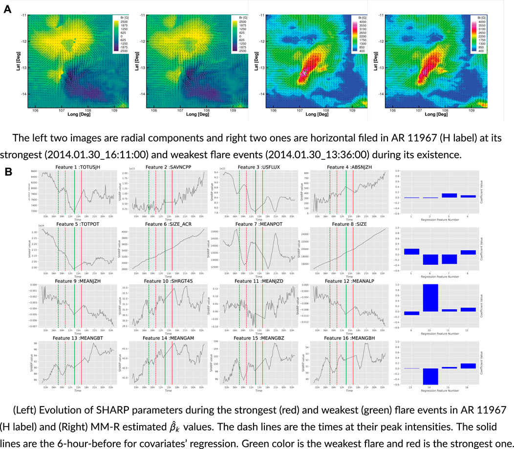
FIGURE 9. The left two images are radial components and right two ones are horizontal filed in AR 11261 (I label) at its strongest (2011.07.30_02:09:00) and weakest flare events (2011.07.30_19:41:00) during its existence. AR 11261 existed from 2011/7/28 to 2011/8/5.

FIGURE 15

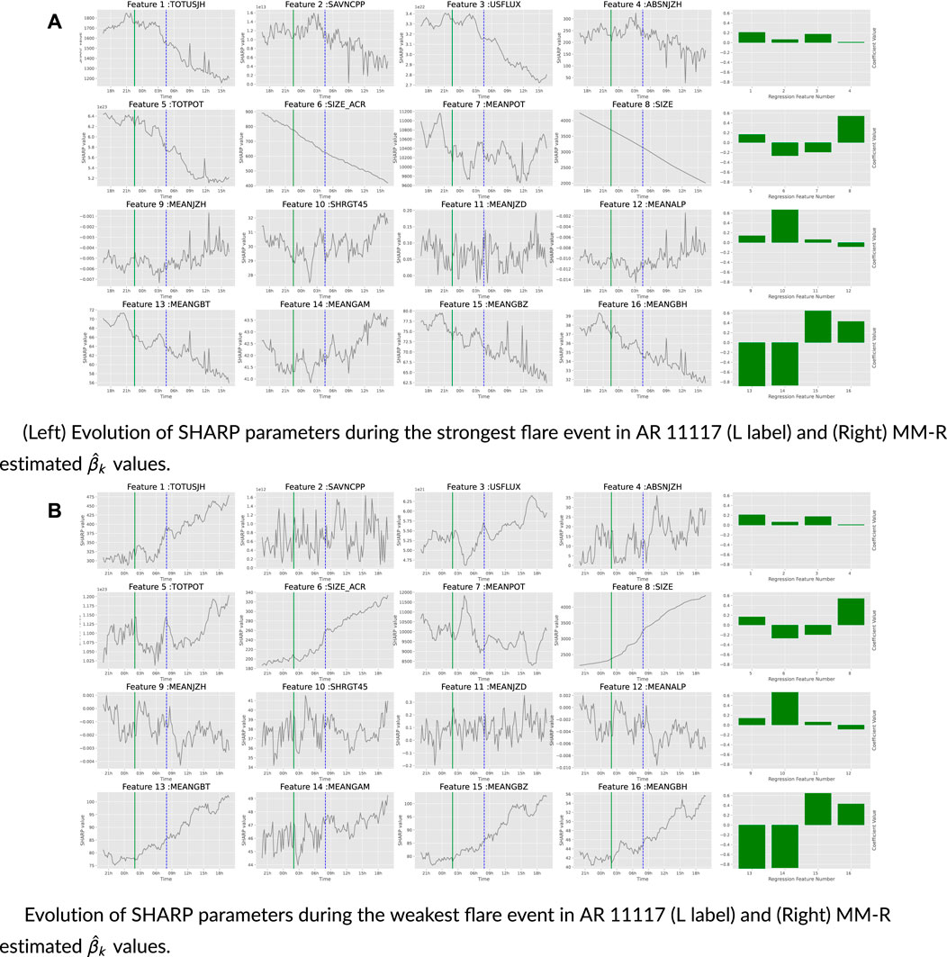
FIGURE 15. SHARP parameters of active region 11,117. AR 11,117 existed from 2010/10/21 to 2010/10/31. (A) (Left) Evolution of SHARP parameters during the strongest flare event in AR 11,117 (L label) and (Right) MM-R-estimated βˆ_k values. (B) (Left) Evolution of SHARP parameters during the weakest flare event in AR 11,117 (L label) and (Right) MM-R-estimated βˆ_k values.

a) The left two images are radial components, and the right two ones are horizontal, filed in AR 11,967 (H label) at its strongest (2014.01.30_16:11:00) and weakest (2014.01.30_13:36:00) flare events during its existence.

b) (Left) Evolution of SHARP parameters during the strongest (red) and weakest (green) flare events in AR 11,967 (H label) and (right) MM-R estimated ${\widehat{\beta }}_k$ values. The dashed lines are the times at their peak intensities. The solid lines are the 6-h-before for covariate regression. Green denotes the weakest flare, and red is the strongest flare.

Data availability statement

All data used in the study, both SHARP parameters and magnetograms are available from Stanford University’s Joint Science Operations Center (JSOC) http://jsoc.stanford.edu/.

Author contributions

BD conducted all the derivations and numerical studies under the guidance of YC and XLN, in collaboration with WM who addressed the interpretation of the physical processes for the flare events. All authors contributed to the article and approved the submitted version.

Funding

YC is funded by NSF DMS 2113397 and NSF PHY 2027555, WM is funded by NSF SWQU Grant PHY-2027555 and NASA LWS Strategic Capability (SCEPTER) 80NSSC22K0892, and XLN is partially supported by the NSF grant DMS-2015361 and a research gift from Wells Fargo.

Conflict of interest

The authors declare that the research was conducted in the absence of any commercial or financial relationships that could be construed as a potential conflict of interest.

Publisher’s note

All claims expressed in this article are solely those of the authors and do not necessarily represent those of their affiliated organizations, or those of the publisher, the editors, and the reviewers. Any product that may be evaluated in this article, or claim that may be made by its manufacturer, is not guaranteed or endorsed by the publisher.

Supplementary material

The Supplementary Material for this article can be found online at: https://www.frontiersin.org/articles/10.3389/fspas.2024.1229092/full#supplementary-material

References

Ahmed, O. W., Qahwaji, R., Colak, T., Higgins, P. A., Gallagher, P. T., and Bloomfield, D. S. (2013). Solar flare prediction using advanced feature extraction, machine learning, and feature selection. Sol. Phys. 283 (1), 157–175. doi:10.1007/s11207-011-9896-1

CrossRef Full Text | Google Scholar

Airoldi, E. M., Blei, D. M., Erosheva, E. A., and Fienberg, S. E. (2014). “Introduction to mixed membership models and methods,” in Handbook of mixed membership models and their applications (Boca Raton: Chapman and Hall/CRC), 37–48.

Google Scholar

Baeke, H., Amaya, J., and Lapenta, G. (2023). Classification of solar flares using data analysis and clustering of active regions.

Google Scholar

Barnes, G., Leka, K. D., Schrijver, C. J., Colak, T., Qahwaji, R., Ashamari, O., et al. (2016). A comparison of flare forecasting methods. I. Results from the all-clear workshop. Astrophysical J. 829 (89), 89. doi:10.3847/0004-637x/829/2/89

CrossRef Full Text | Google Scholar

Bishop, C. M. (2006). Pattern recognition and machine learning (information science and statistics). Berlin, Heidelberg: Springer-Verlag.

Google Scholar

Bobra, M. G., and Couvidat, S. (2015). Solar flare prediction using SDO/HMI vector magnetic field data with a machine-learning algorithm. Astrophysical J. Astrophysical J. 798 (135), 135. doi:10.1088/0004-637x/798/2/135

CrossRef Full Text | Google Scholar

Bobra, M. G., Sun, X., Hoeksema, J. T., Turmon, M., Liu, Y., Hayashi, K., et al. (2014). The helioseismic and magnetic imager (HMI) vector magnetic field pipeline: SHARPs –Space-Weather HMI active region patches. Sol. Phys. 289 (9), 3549–3578. doi:10.1007/s11207-014-0529-3

CrossRef Full Text | Google Scholar

Camporeale, E. (2019). The challenge of machine learning in space weather: nowcasting and forecasting. Space weather. 17 (8), 1166–1207. doi:10.1029/2018sw002061

CrossRef Full Text | Google Scholar

Carroll, R. J., and Pederson, S. (1993). On robustness in the logistic regression model. J. R. Stat. Soc. Ser. B Methodol. 55 (3), 693–706. doi:10.1111/j.2517-6161.1993.tb01934.x

CrossRef Full Text | Google Scholar

Chen, Y., Manchester, W. B., Hero, A. O., Toth, G., DuFumier, B., Zhou, T., et al. (2019). Identifying solar flare precursors using time series of SDO/HMI images and SHARP parameters. Space weather. 17 (10), 1404–1426. doi:10.1029/2019sw002214

CrossRef Full Text | Google Scholar

Chintzoglou, G., Zhang, J., Cheung, M. C. M., and Kazachenko, M. (2019). The origin of major solar activity: collisional shearing between nonconjugated polarities of multiple bipoles emerging within active regions. Astrophysical J. 871 (1), 67. doi:10.3847/1538-4357/aaef30

CrossRef Full Text | Google Scholar

Colak, T., and Qahwaji, R. (2008). Automated McIntosh-based classification of sunspot groups using MDI images. Sol. Phys. 248, 277–296. doi:10.1007/s11207-007-9094-3

CrossRef Full Text | Google Scholar

Dempster, A. P., Laird, N. M., and Rubin, D. B. (1977). Maximum likelihood from incomplete data via the EM algorithm. J. R. Stat. Soc. Ser. B Methodol. 39 (1), 1–22. doi:10.1111/j.2517-6161.1977.tb01600.x

CrossRef Full Text | Google Scholar

Durán, J. S. C., Lagg, A., Solanki, S. K., and van Noort, M. (2020). Detection of the strongest magnetic field in a sunspot light bridge. Astrophysical J. 895 (2), 129. doi:10.3847/1538-4357/ab83f1

CrossRef Full Text | Google Scholar

Fang, F., Manchester, W., Abbett, W. P., and van der Holst, B. (2010). Simulation of flux emergence from the convection zone to the corona. Astrophysical J. 714 (2), 1649–1657. doi:10.1088/0004-637x/714/2/1649

CrossRef Full Text | Google Scholar

Field, C., and Smith, B. (1994). Robust estimation: a weighted maximum likelihood approach. Int. Stat. Review/Rev. Int. Stat. 62 (3), 405–424. doi:10.2307/1403770

CrossRef Full Text | Google Scholar

Garcia, H. A. (1994). Temperature and emission measure from goes soft X-ray measurements. Sol. Phys. 154 (2), 275–308. doi:10.1007/BF00681100

CrossRef Full Text | Google Scholar

Goutte, C., and Gaussier, E. (2005). “A probabilistic interpretation of precision, recall and F-score, with implication for evaluation,” in Advances in information retrieval berlin. Editors D. E. Losada, and J. M. Fernández-Luna (Heidelberg: Springer Berlin Heidelberg), 345–359.

CrossRef Full Text | Google Scholar

Green, L. M., Török, T., Vršnak, B., Manchester, W., and Veronig, A. (2018). The origin, early evolution and predictability of solar eruptions. Space Sci. Rev. 214 (1), 46. doi:10.1007/s11214-017-0462-5

CrossRef Full Text | Google Scholar

Huang, X., Wang, H., Xu, L., Liu, J., Li, R., and Dai, X. (2018). Deep learning based solar flare forecasting model. I. Results for line-of-sight magnetograms. Astrophysical J. 856 (1), 7. doi:10.3847/1538-4357/aaae00

CrossRef Full Text | Google Scholar

Janvier, M., Mzerguat, S., Young, P. R., É, B., Manou, A., Pelouze, G., et al. (2023). A multiple spacecraft detection of the 2 April 2022 M-class flare and filament eruption during the first close Solar Orbiter perihelion. Astronomy Astrophysics 677, A130. doi:10.1051/0004-6361/202346321

CrossRef Full Text | Google Scholar

Jiang, C., Feng, X., Wu, S. T., and Hu, Q. (2012). Study of the three-dimensional coronal magnetic field of active region 11117 around the time of a confined flare using a data-driven CESE-MHD model. Astrophysical J. 759 (2), 85. doi:10.1088/0004-637x/759/2/85

CrossRef Full Text | Google Scholar

Jiang, C., Wu, S., Feng, X., Jiang, Y., and Warren, A. (2016). Morphology and molecular phylogeny of two freshwater peritrich ciliates, epistylis chlorelligerum shen 1980 and epistylis chrysemydis bishop and jahn 1941 (Ciliophora, peritrichia). Front. Astronomy Space Sci. 3, 16–26. doi:10.1111/jeu.12243

PubMed Abstract | CrossRef Full Text | Google Scholar

Jiang, C. W., Feng, X. S., Wu, S. T., and Hu, Q. (2017). A magnetic bald-patch flare in solar active region 11117. Res. Astronomy Astrophysics 17 (9), 093. doi:10.1088/1674-4527/17/9/93

CrossRef Full Text | Google Scholar

Jiao, Z., Sun, H., Wang, X., Manchester, W., Gombosi, T., Hero, A., et al. (2020). Solar flare intensity prediction with machine learning models. Space weather. 18 (7), e2020SW002440. doi:10.1029/2020sw002440

CrossRef Full Text | Google Scholar

Joshi, A. D., Forbes, T. G., Park, S. H., and Cho, K. S. (2015). A trio of confined flares in AR 11087. Astrophysical J. 798 (2), 97. doi:10.1088/0004-637x/798/2/97

CrossRef Full Text | Google Scholar

Joshi, N. C., Joshi, B., and Mitra, P. K. (2021). Evolutionary stages and triggering process of a complex eruptive flare with circular and parallel ribbons. Mon. Notices R. Astronomical Soc. 501 (4), 4703–4721. doi:10.1093/mnras/staa3480

CrossRef Full Text | Google Scholar

Kawabata, Y., Inoue, S., and Shimizu, T. (2017). Non-potential field formation in the X-shaped quadrupole magnetic field configuration. Astrophysical J. 842 (2), 106. doi:10.3847/1538-4357/aa71a0

CrossRef Full Text | Google Scholar

Koller, D., and Friedman, N. (2009). Probabilistic graphical models: principles and techniques. United States: MIT press.

Google Scholar

Landa, V., and Reuveni, Y. (2022). Low-dimensional convolutional neural network for solar flares GOES time-series classification. Astrophysical J. Suppl. Ser. 258 (1), 12. doi:10.3847/1538-4365/ac37bc

CrossRef Full Text | Google Scholar

Leka, K. D., and Barnes, G. (2018). “Chapter 3 - solar flare forecasting: present methods and challenges,” in Extreme events in geospace. Editor N. Buzulukova (Amsterdam, Netherlands: Elsevier), 65–98.

CrossRef Full Text | Google Scholar

Liu, C., Deng, N., Lee, J., Wiegelmann, T., Jiang, C., Dennis, B. R., et al. (2014). Three-dimensional magnetic restructuring in two homologous solar flares in the seismically active NOAA AR 11283. Astrophysical J. 795 (2), 128. doi:10.1088/0004-637x/795/2/128

CrossRef Full Text | Google Scholar

Liu, H., Liu, C., Wang, J. T. L., and Wang, H. (2019). Predicting solar flares using a Long short-term memory network. Astrophysical J. 877 (2), 121. doi:10.3847/1538-4357/ab1b3c

CrossRef Full Text | Google Scholar

Liu, R. (2020). Magnetic flux ropes in the solar corona: structure and evolution toward eruption. Res. Astronomy Astrophysics 20 (10), 165. doi:10.1088/1674-4527/20/10/165

CrossRef Full Text | Google Scholar

Liu, R., Kliem, B., Titov, V. S., Chen, J., Wang, Y., Wang, H., et al. (2016). Structure, stability, and evolution of magnetic flux ropes from the perspective of magnetic twist. Astrophysical J. 818 (2), 148. doi:10.3847/0004-637x/818/2/148

CrossRef Full Text | Google Scholar

Maloney, S. A., and Gallagher, P. T. (2018). “Sunspot group classification using neural networks,” in Catalyzing solar connections, 92.

Google Scholar

Manchester, I. W., Gombosi, T., DeZeeuw, D., and Fan, Y. (2004). Eruption of a buoyantly emerging magnetic flux rope. Astrophysical J. 610 (1), 588–596. doi:10.1086/421516

CrossRef Full Text | Google Scholar

Manchester, W. (2003). Buoyant disruption of magnetic arcades with self-induced shearing. J. Geophys. Res. (Space Phys.) 108 (A4), 1162. doi:10.1029/2002ja009252

CrossRef Full Text | Google Scholar

Markatou, M., Basu, A., and Lindsay, B. G. (1998). Weighted likelihood equations with bootstrap root search. J. Am. Stat. Assoc. 93 (442), 740–750. doi:10.1080/01621459.1998.10473726

CrossRef Full Text | Google Scholar

McLachlan, G. J., and Peel, D. (2000). “Finite mixture models,” in Probability and statistics – applied probability and statistics section. 299 (New York: Wiley).

Google Scholar

NASA (2003). Halloween Storms of still the scariest. United States: NASA.

Google Scholar

Nguyen, T. T., Willis, C. P., Paddon, D. J., and Nguyen, H. S. (2004). “On learning of sunspot classification,” in Intelligent information processing and web mining. Editors M. A. Kłopotek, S. T. Wierzchoń, and K. Trojanowski (Berlin, Heidelberg: Springer Berlin Heidelberg), 59–68.

CrossRef Full Text | Google Scholar

Romano, P., Elmhamdi, A., Falco, M., Costa, P., Kordi, A. S., Al-Trabulsy, H. A., et al. (2018). Homologous white light solar flares driven by photospheric shear motions. Astrophysical J. Lett. 852 (1), L10. doi:10.3847/2041-8213/aaa1df

CrossRef Full Text | Google Scholar

Sarkar, R., Srivastava, N., and Veronig, A. M. (2019). Lorentz force evolution reveals the energy build-up processes during recurrent eruptive solar flares. Astrophysical J. Lett. 885 (1), L17. doi:10.3847/2041-8213/ab4da2

CrossRef Full Text | Google Scholar

Schou, J., Scherrer, P. H., Bush, R. I., Wachter, R., Couvidat, S., Rabello-Soares, M. C., et al. (2012). Design and ground calibration of the helioseismic and magnetic imager (HMI) instrument on the solar Dynamics observatory (SDO). Sol. Phys. 275 (1-2), 229–259. doi:10.1007/s11207-011-9842-2

CrossRef Full Text | Google Scholar

Smith, M. C., Jones, A. R., and Sandoval, L. (2018). “Automating the McIntosh classification system using machine learning,” in AGU Fall Meeting Abstracts, Washington, DC, December 10 – 14 2018, SM31D–3526.

Google Scholar

Solovev, A. A., Abramov-Maximov, V. E., Borovik, V. N., Opeikina, L. V., and Tlatov, A. G. (2019). Features of evolution of the magnetic field gradient in solar active region before a strong flare. Astronomical Astrophysical Trans. 31 (2), 89–102. doi:10.17184/eac.2967

CrossRef Full Text | Google Scholar

Song, H., Tan, C., Jing, J., Wang, H., Yurchyshyn, V., and Abramenko, V. (2009). Statistical assessment of photospheric magnetic features in imminent solar flare predictions. Sol. Phys. 254 (1), 101–125. doi:10.1007/s11207-008-9288-3

CrossRef Full Text | Google Scholar

Sui, L., Holman, G. D., and Dennis, B. R. (2004). Evidence for magnetic reconnection in three homologous solar flares observed by RHESSI. Astrophysical J. 612 (1), 546–556. doi:10.1086/422515

CrossRef Full Text | Google Scholar

Thalmann, J. K., Veronig, A., and Su, Y. (2016). Temporal and spatial relationship of flare signatures and the force-free coronal magnetic field. Astrophysical J. 826 (2), 143. doi:10.3847/0004-637x/826/2/143

CrossRef Full Text | Google Scholar

Titov, V. S., Mikic, Z., Török, T., Linker, J. A., and Panasenco, O. (2010). Sympathetic eruptions. I. Magnetic topology of the source-surface background field. Astrophysical J. 759 (1), 70. doi:10.1088/0004-637x/759/1/70

CrossRef Full Text | Google Scholar

Titterington, D. M., Smith, A. F. M., and Makov, U. E. (1985). Statistical analysis of finite mixture distributions. New York: Wiley.

Google Scholar

Wang, X., Chen, Y., Toth, G., Manchester, W. B., Gombosi, T. I., Hero, A. O., et al. (2020). Predicting solar flares with machine learning: investigating solar cycle dependence. Astrophysical J. 895 (1), 3. doi:10.3847/1538-4357/ab89ac

CrossRef Full Text | Google Scholar

Ward, M. I. (2001). The role of nonlinear alfvén waves in shear formation during solar magnetic flux emergence. Astrophysical J. 547 (1), 503–519. doi:10.1086/318342

CrossRef Full Text | Google Scholar

Ward, M. I. (2007). Solar atmospheric dynamic coupling due to shear motions driven by the Lorentz force. Astrophysical J. 666 (1), 532–540. doi:10.1086/520493

CrossRef Full Text | Google Scholar

Wu, C. F. J. (1983). On the convergence properties of the EM algorithm. Ann. Statistics 11 (1), 95–103. doi:10.1214/aos/1176346060

CrossRef Full Text | Google Scholar

Ye, Y., Korsós, M. B., and Erdélyi, R. (2018). Detailed analysis of dynamic evolution of three Active Regions at the photospheric level before flare and CME occurrence. Adv. Space Res. 61 (2), 673–682. doi:10.1016/j.asr.2017.09.038

CrossRef Full Text | Google Scholar

Yu, D., Huang, X., Wang, H., and Cui, Y. (2009). Short-Term solar flare prediction using a sequential supervised learning method. Sol. Phys. 255 (1), 91–105. doi:10.1007/s11207-009-9318-9

CrossRef Full Text | Google Scholar

Yuan, Y., Shih, F. Y., Jing, J., and Wang, H. M. (2010). Automated flare forecasting using a statistical learning technique. Res. Astronomy Astrophysics 10 (8), 785–796. doi:10.1088/1674-4527/10/8/008

CrossRef Full Text | Google Scholar