Improved models for estimating sporadic-E intensity from GNSS radio occultation measurements

Several models for estimating sporadic-E intensity from Global Navigation Satellite System (GNSS) radio occultation (RO) observation have previously been developed using a single perturbation or intensity parameter, such as phase-based total electron content (TEC) or the amplitude-based S₄ index. Here, we outline two new models that use a combination of phase and amplitude parameters for the L₁ and L₂ signals. These models show a significant improvement over the baseline models used for comparison. Furthermore, the GNSS-RO parameters are compared with several different ionosonde intensity parameters including the direct foEs and fbEs measurements along with the metallic-ion based fo$\mathit{\mu }$Es and fb$\mathit{\mu }$Es parameters which account for the background E-region density. Interestingly, the phase-based ${\mathit{\sigma }}_{\mathit{\varphi }}$ scintillation index shows the strongest correlation to foEs and fbEs while amplitude-based S₄ shows the strongest correlation to fo$\mathit{\mu }$Es and fb$\mathit{\mu }$Es. While the metallic-ion based fo$\mathit{\mu }$Es and fb$\mathit{\mu }$Es parameters are physically ideal for GNSS-RO observations, we show difficulties in practical implementation due to the reliance on a background E-region density estimate using a model such as the International Reference Ionosphere (IRI). Ultimately, we provide two improved sporadic-E intensity models that can be used for future GNSS-RO based studies along with a recommendation to compare against the ionosonde-based foEs parameter.

1 Introduction

Sporadic-E (E_s) is characterized by an unusually dense plasma at E-region altitudes caused by elevated metallic-ion densities from meteor deposits converged through neutral wind shears (Whitehead, 1989; Mathews, 1998; Haldoupis, 2011; Shinagawa et al., 2021). These enhanced ion layers can significantly affect radio propagation, especially high-frequency (HF) skywaves (McNamara, 1991; Fabrizio, 2013) and Global Navigation Satellite System (GNSS) signals used for Low Earth Orbit (LEO) satellite position and timing (Yue et al., 2016). Therefore, understanding both the global occurrence rates (Smith, 1957; Chu et al., 2014; Arras and Wickert, 2018; Hodos et al., 2022) and E_s intensities [i.e., peak ion densities; Yu et al. (2020); Merriman et al. (2021); Yu et al. (2022)] are vital to many aspects of our modern civilization.

While ionosondes provide direct measurements of E_s intensities in terms of the peak blanketing frequency, fbEs, and the peak frequency of the ordinary mode return, foEs, ionosondes are inherently land-locked with a sparse distribution throughout the globe (e.g., see Digisonde stations at https://giro.uml.edu/). For this reason, we must use indirect measurements of E_s intensities obtained through GNSS radio occultation (RO) to obtain truly global coverage (Wu et al., 2005; Yeh et al., 2014; Tsai et al., 2018; Niu et al., 2019; Yu et al., 2019; Luo et al., 2021). However, the indirect nature of GNSS-RO observations makes it difficult to accurately extract E_s parameters, resulting in large uncertainties and ambiguities (Gooch et al., 2020; Carmona et al., 2022).

Specifically, many GNSS-RO techniques have been proposed to extract sporadic-E intensities from phase (Hocke et al., 2001; Niu et al., 2019; Gooch et al., 2020) and amplitude (Arras and Wickert, 2018; Yu et al., 2020) perturbations using direct ionosonde measurements for validation. The phase techniques referenced above rely on total electron content (TEC) calculations using L₁ (1,575.41 MHz) and L₂ (1,227.60 MHz) phase-based perturbations while the amplitude-based techniques use an L₁ scintillation index such as S₄ to estimate E_s intensities. No technique that we are aware of uses both amplitude and phase information for intensity estimates. Furthermore, phase perturbation techniques will be affected by phase scintillation (σ_ϕ) for stronger E_s layers (Emmons et al., 2022), and the amplitude scintillation indices have been shown to plateau for stronger layers (Stambovsky et al., 2021).

To further complicate matters, it is unclear which ionosonde-based E_s intensity measurement is appropriate for comparison against GNSS-RO observations. Ionosondes provide two commonly used E_s intensity parameters: fbEs and foEs. The fbEs typically correspond to more uniform layers that block HF signals from penetrating with frequencies below the fbEs, while the foEs correspond to the peak plasma frequency measured in patchy or cloudy layers (Reddy and Mukunda Rao, 1968). The GNSS-RO community is generally divided on which parameter to use for comparison, with some using foEs as the validation parameter (Hocke et al., 2001; Niu et al., 2019; Yu et al., 2020) and others using fbEs (Arras and Wickert, 2018; Gooch et al., 2020). Furthermore, GNSS-RO measurements have been shown to actually measure the metallic-ion density perturbation from the background E-region plasma density, which requires a conversion of foEs/fbEs to foμEs/fbμEs as outlined by Haldoupis (2019). These metallic-ion foμEs and fbμEs parameters are calculated by subtracting the electron density of the background E region from the total ion density derived from foEs or fbEs, such that the metallic-ion density is obtained for the E_s layer. No GNSS-RO technique that we are aware of uses these perturbation-based metallic-ion parameters for comparison.

In this study, we develop two improved models for sporadic-E intensity using a combination of L₁ and L₂ amplitude and phase data in comparison with ionosonde observations. Additionally, we create separate models for foEs, fbEs, foμEs, and fbμEs to determine which parameter shows the strongest agreement with ionosonde observations. The results outlined below show a significant improvement in the E_s intensity estimates from GNSS-RO observations, which can be used to refine global empirical models and provide valuable near-real-time information to radio operators.

2 Materials and methods

COSMIC-I 50 Hz atmPhs data obtained from the COSMIC Data Analysis and Archive Center (CDAAC; https://cdaac-www.cosmic.ucar.edu/cdaac/index.html) from 2010 to 2017 are used for GNSS-RO observations. Since GNSS-RO methods do not provide a direct measurement of sporadic-E intensity, a separate dataset must be used for validation. Here, we use ionosonde foEs and fbEs measurements obtained through the Digital Ionogram DataBase (DIDBase; https://giro.uml.edu/didbase/) as the validation data set. Due to the large number of ionograms analyzed in this study, we rely on ionograms automatically scaled by Automatic Real-Time Ionogram Scaler with True height software, version 5 [ARTIST-5; (Galkin and Reinisch 2008)]. Most Digisondes incorporated ARTIST-5 around 2010, which is why RO data before 2010 are not included in this comparison. No Confidence Score (CS) threshold was implemented on the automatically scaled ionograms due to the fact that the CS grading criteria is based on standard electron density profiles that deduct points for irregularities like sporadic-E (Galkin et al., 2013). Requiring high CS values can unintentionally remove ionograms with reliable sporadic E measurements, which would be detrimental to this analysis.

Uncertainties in ARTIST-5 predictions have recently been quantified by Stankov et al. (2023) through a comparison with manually scaled ionograms. They found an foEs error bound of [−0.80, 0.35] MHz for the ARTIST-5 estimates minus manually scaled values. This interval contains 95% of the ionograms in the comparison, providing an uncertainty range for the validation dataset used in the present study.

Figure 1 shows example ionograms and the corresponding GNSS-RO amplitude and phase profiles measured with and without sporadic-E present. The amplitude scintillation and phase perturbation caused by the sporadic-E layer is immediately obvious, especially when compared against the measurements without sporadic-E. To limit the spatial and temporal difference between ionosonde and GNSS-RO measurements, RO tangent points must be within 30 min and 50 km of an ionogram that measures sporadic-E. This spatial extent corresponds to half of the 100 km median length of sporadic-E layers as observed by Maeda and Heki (2015), such that a layer directly over an ionosonde can be observed within a 50 km radius. While reducing the comparison distance causes a reduction in the overall number of concurrent measurements, it allows for more confidence in the fact that both the ionosonde and occultation are measuring the same layer. We also examined larger comparison distances (results not shown), which produced similar results with larger uncertainties caused by measurements of separate E_s clouds or RO observations that miss the clouds altogether. All concurrent (within 30 min and 50 km) COSMIC-1 GNSS-RO and DIDBase ionosonde measurements throughout the globe during 2010–2017 are used for this analysis.

FIGURE 1

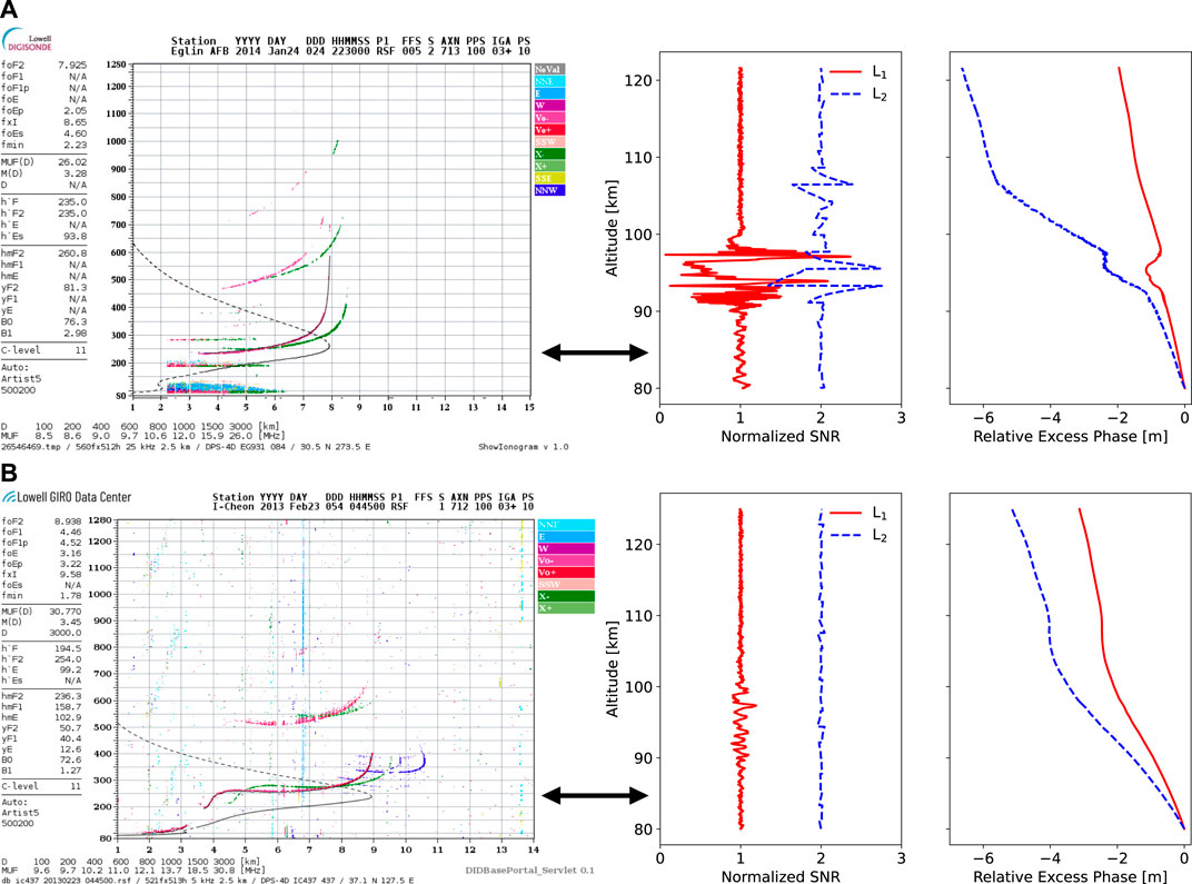
FIGURE 1. Ionograms and corresponding GNSS-RO amplitude (normalized SNR) and relative excess phase data (A) with sporadic-E present and (B) without sporadic-E. The normalized L₂ SNR is shifted horizontally to improve readability. Note the strong SNR scintillation and phase perturbation caused by the sporadic-E layer near 95 km in the top row. The CDAAC descriptors displayed here are (A) atmPhs_C006.2014.024.22.34.G18_2013.3520_nc and (B) atmPhs_C002.2013.054.04.43.G22_2013.3520_nc.

As a baseline for comparison, two commonly used RO techniques for estimating sporadic-E intensity are included in the results: the S₂ amplitude scintillation-based technique from Arras and Wickert (2018) and the total electron content (TEC) based technique from Gooch et al. (2020). Note that we use S₂ for the amplitude scintillation index here instead of the S₄ intensity scintillation index following the Briggs and Parkin (1963) definition with COSMIC-1 signal-to-noise-ratio (SNR [V/V]) corresponding to the signal amplitude. The Arras and Wickert (2018) model was selected instead of the updated (Yu et al., 2020) S₄ model, as we calculate all parameters directly from the CDAAC 50 Hz atmPhs files, while the Yu et al. (2020) technique uses scnLv1 files that are calculated in a slightly different manner (see Syndergaard, 2006). After the S₂ is calculated using a sliding window of 50 points (one second in time for 50 Hz atmPhs data), the empirical conversion fEs [MHz] = 3.8×S₂ + 2.0 is used to calculate the sporadic-E intensity fEs. Throughout this comparison, we use fEs for the GNSS-RO derived intensities instead of foEs, fbEs, etc., as it is unclear which (if any) of the ionosonde specific parameters is measured by RO.

The Gooch et al. (2020) technique uses the L₁ and L₂ phases to calculate a TEC, which is then detrended with a Savitzky-Golay (Savitzky and Golay, 1964) filter using a 25 km window. The detrended TEC is then smoothed using a 1 km Savitzky-Golay filter, and the final TEC perturbation is divided by an effective path length of 176 km for an assumed vertical thickness of 0.6 km (Ahmad, 1999) to obtain an electron density for the layer. This technique provides a physically straightforward approach to estimate layer intensities. However, it relies on the assumption of an unknown path length (horizontal length) that can introduce a large uncertainty into the calculations.

In addition to the S₂ and TEC calculations discussed above, a variety of scintillation and perturbation parameters are calculated for each RO crossing to examine previously unexplored relationships with sporadic-E intensity. These parameters include the amplitude scintillation index S₄, the standard deviation of the nondetrended (measured) excess phase σ_ϕ, and the phase perturbation Δϕ calculated from a 25 km Savitzky-Golay filter used for detrending. All these parameters are calculated for both the L₁ and L₂ frequencies. A list of the parameters and additional details on the calculations are displayed in Table 1. The size of the sliding windows and the number of detrending iterations (zero or one) for S₄, σ_ϕ, and Δϕ were optimized to improve correlations with the ionosonde foEs and fbEs data.

TABLE 1

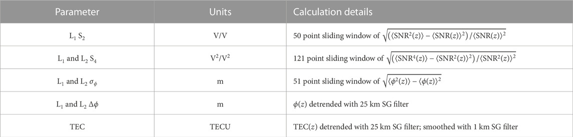
TABLE 1. Details on the GNSS-RO scintillation and perturbation parameters calculated from 50 Hz atmPhs observations of sporadic-E. Here, SNR is the signal amplitude, ϕ is the excess phase, z is the altitude, SG stands for Savitzky-Golay, and ⟨ ⟩ denotes the average over the specified window. The S₂ and S₄ formulas shown here follow Briggs and Parkin (1963) for COSMIC-1 SNR representing the signal amplitude.

IRI-2016 (Bilitza et al., 2017) is used to estimate the background E-region ion density required for foμEs and fbμEs calculations. Following the procedure described by Haldoupis, (2019), the background E-region ion density at the sporadic-E altitude is estimated by IRI and is subtracted from the foEs (fbEs) to obtain the metallic-ion density, which can be converted to a frequency foμEs (fbμEs). While ionosondes provide the virtual height of the sporadic-E layer, h’Es, the actual height can be estimated by integrating the group index of refraction over altitude to find the actual height corresponding to the measured virtual height [see further description in Gooch et al. (2020)]. The actual height is calculated from the IRI electron density profile (EDP), then the background E-region ion density is set to the IRI density at the calculated E_s actual height. While this places a strong reliance on IRI predictions for the metallic-ion intensity parameters, we use IRI instead of ionosonde derived EDPs for two reasons: first, blanketing sporadic-E can block the ionosonde returns from the background E-region completely, such that the Digisonde EDP inversion process relies on climatology. Second, to extend this approach to locations without ionosondes in application of the GNSS-RO techniques for global climatology, etc., a model will be required as no local EDP measurements will be available.

The foμEs and fbμEs parameters are derived from metallic-ion density perturbations to the background E-region ionosphere (Haldoupis, 2019). Physically, this perturbation is vitally important for quantifying the impacts of E_s layers on GNSS-RO signals, as the primary factor in the signal perturbation magnitude is the vertical index of refraction (plasma density) gradient (Wu, 2006). The background E-region density gradient is too small to cause significant diffraction in the GNSS-RO signals, while vertically thin sporadic-E layers provide sufficiently large vertical density gradients (see Figure 1). Therefore, the background E-region contribution is insignificant when quantifying the strength of sporadic-E layers for GNSS-RO signal perturbations, and the background densities should be removed to provide the metallic-ion based foμEs and fbμEs parameters. As discussed in Sections 3 and 4, while the physical reasoning behind this conversion makes sense for GNSS-RO applications, the practical implementation is rather difficult.

3 Results

3.1 Relationship between E_s intensity parameters

GNSS-RO signals are prone to significant phase perturbations from E_s layers, which cause diffraction patterns that are dependent on the vertical thickness and total phase contribution (Zeng and Sokolovskiy, 2010; Stambovsky et al., 2021; Emmons et al., 2022). The total phase contribution depends on both the metallic-ion density and the horizontal length of the layer through which the signal crosses. Since the normal E-region varies relatively slowly with altitude (in comparison with E_s layers), the phase contribution to the plane-wave GNSS-RO signal is nearly uniform over a small altitude range and does not result in significant perturbations or diffraction. In contrast, the relatively thin vertical thickness of sporadic-E [∼1.5 km; Zeng and Sokolovskiy (2010)] acts like a negative lens capable of producing significant perturbations to the RO signals. Therefore, as outlined in Haldoupis (2019), GNSS-RO measurements are sensitive to the metallic-ion density in E_s, not to the total ion density that includes the background E-region.

In terms of E_s intensity parameters, this metallic-ion density can be estimated from foEs and fbEs through conversion to foμEs and fbμEs, which removes this background E-region contribution. Physically, this argument suggests that the GNSS-RO fEs intensity estimates should only be compared to ionosonde derived foμEs and fbμEs. However, in practice, our reliance on models or low-confidence EDP estimates from ionosondes (because of the presence of sporadic-E) makes it difficult to obtain accurate background E-region densities. This point will be discussed in more detail later, but first we focus on the relationships between these different intensity parameters.

Figure 2 shows the relationships between the different E_s intensity parameters. A lower limit of 1 MHz was placed on the foμEs and fbμEs values as the perturbation to GNSS-RO signals would be minor for these weak layers. The different intensity parameters generally show a strong correlation in terms of Spearman’s ρ used throughout this study for potentially nonlinear trends. As expected, the foμEs and fbμEs values are lower than the foEs and fbEs values, with a collection of data points near the 1:1 line corresponding to weak background E-region densities measured at night. Here, night corresponds to a solar zenith angle greater than or equal to 90°, which is roughly 40% of the E_s measurements used in this analysis. Calculated linear slopes of 0.8 and 0.6 are found for the foEs to foμEs and fbEs to fbμEs conversions, respectively.

FIGURE 2

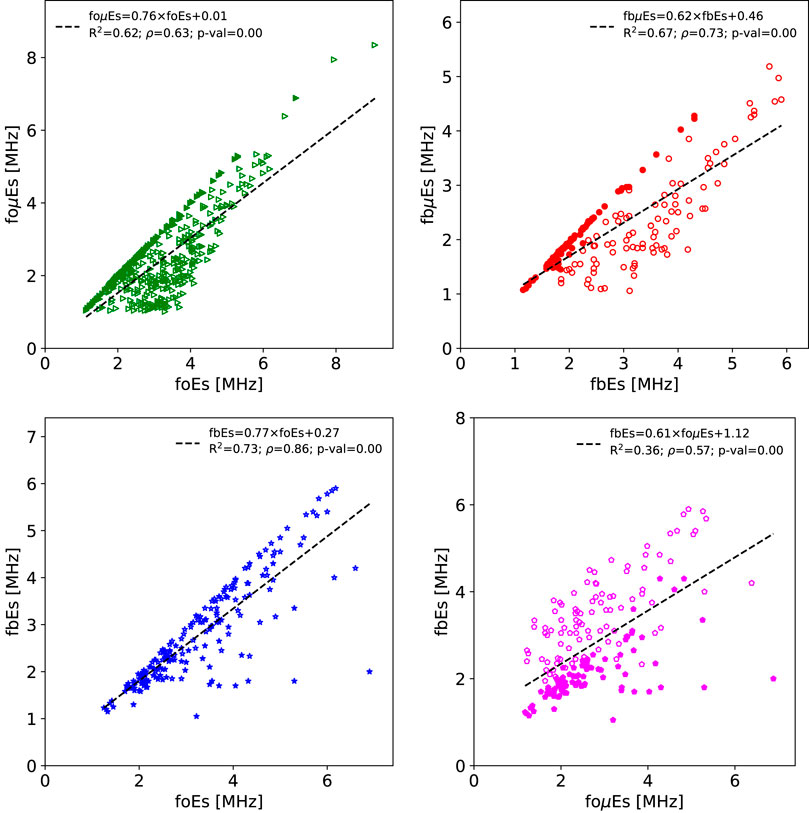
FIGURE 2. Comparisons of the ionosonde derived E_s intensity parameters. The foEs and fbEs are obtained directly from ionosonde measurements while foμEs and fbμEs are the metallic-ion parameters derived following (Haldoupis, 2019). The unfilled markers correspond to daytime measurements while the filled markers designate nighttime measurements.

For ionosonde measurements with both foEs and fbEs measured, the relationship shows that most fbEs values are close in magnitude to the foEs values. However, there are several ionograms that show strong foEs with weak fbEs. This results in a linear fit with a slope of 0.8 to convert foEs to fbEs.

In an attempt to determine whether fbEs could be used as a proxy for foμEs, the two parameters were compared. From the results, we see that the relationship is relatively weak with a linear fit that results in a slope of 0.6 and an R² of 0.4. This indicates that fbEs should not be used as an easy-to-obtain proxy for foμEs.

The nontrivial relationships between the different E_s intensity parameters make it difficult to choose a single parameter for comparison with GNSS-RO observations. While the metallic-ion parameters are physically more appropriate, the additional uncertainty introduced by model estimates of the background E-region may weaken the overall relationships with RO derived parameters. Therefore, we decided to include all four intensity parameters in our model development to determine which of the parameters is the most practical to use when comparing with GNSS-RO observations.

3.2 GNSS-RO parameters vs. ionosonde intensity parameters

Ionosonde intensity parameters are displayed against the GNSS-RO scintillation and perturbation parameters in Figures 3–6. Thresholds are placed on the GNSS-RO parameters to remove outliers for quality control, and the values for each parameter are displayed in Table 2. These phase-based thresholds were determined from visual inspection of the results, but a future evaluation of the values using simulated profiles may provide an improved approach with a physical basis. For amplitude scintillation, strong signal focusing can result in S₄ saturation with indices around 1.5 (Singleton, 1970), which is below the 2.0 threshold implemented here.

FIGURE 3

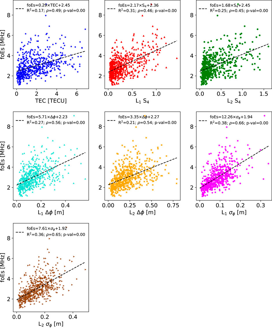
FIGURE 3. Ionosonde derived foEs as a function of GNSS-RO scintillation and perturbation parameters. Note the relatively strong correlation with ${\mathit{\sigma }}_{\mathit{\varphi }}$.

FIGURE 4

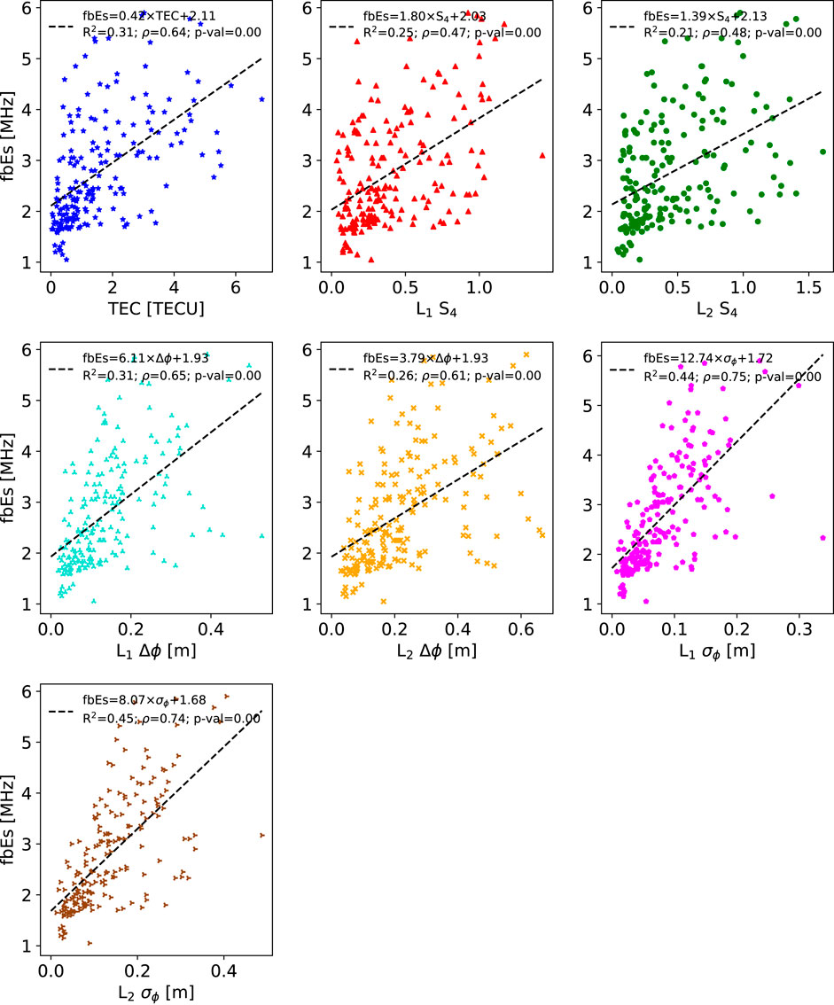
FIGURE 4. Same as Figure 3 but for fbEs. Similar to foEs, there is a relatively strong correlation with ${\mathit{\sigma }}_{\mathit{\varphi }}$.

FIGURE 5

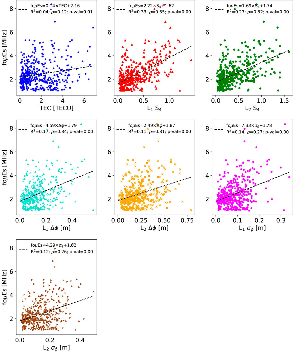
FIGURE 5. Same as Figure 3 but for foμEs. Note the moderate correlation with S₄ and weak correlation with TEC.

FIGURE 6

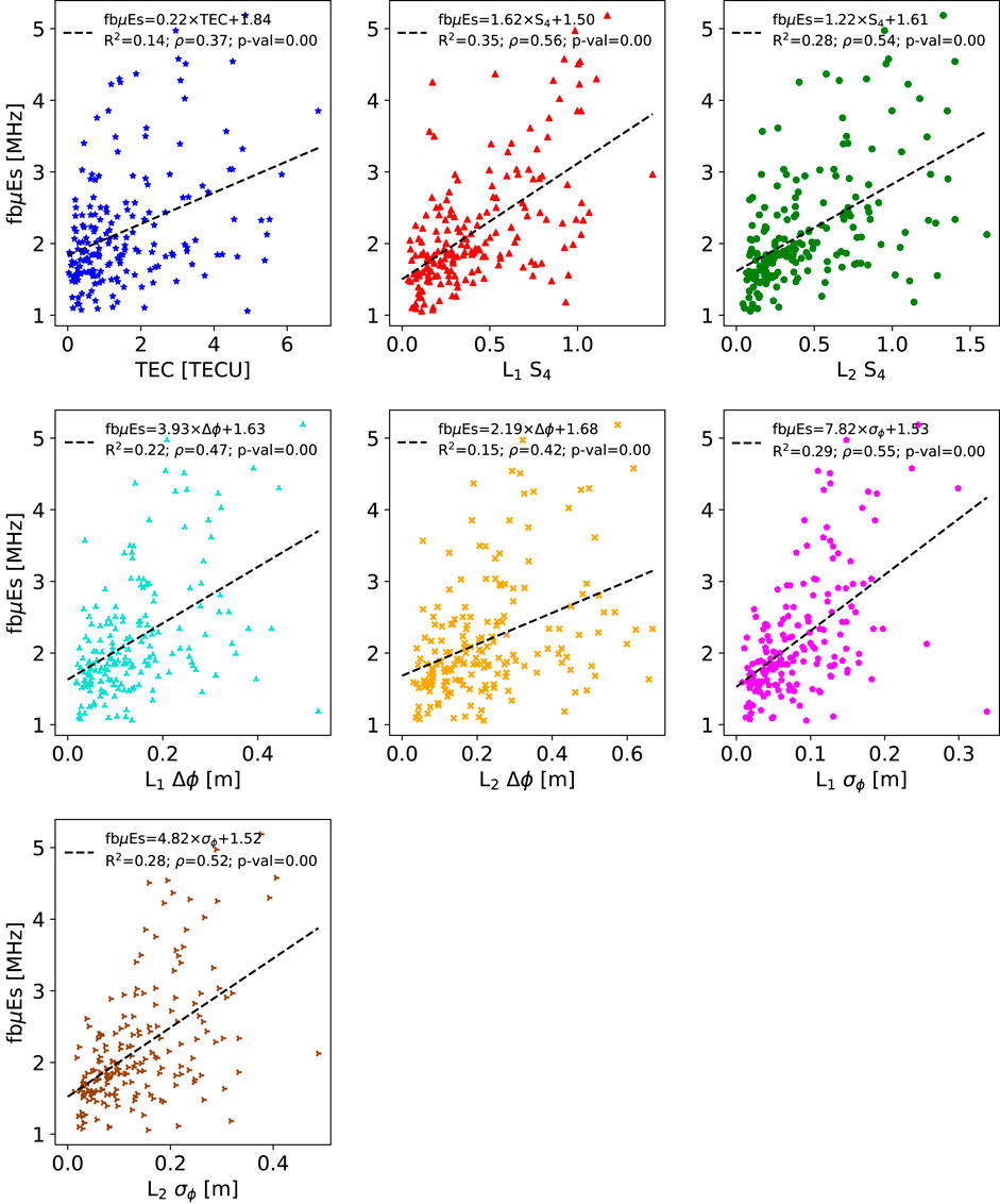
FIGURE 6. Same as Figure 3 but for fbμEs. Note the moderate correlations with S₄ and ${\mathit{\sigma }}_{\mathit{\varphi }}$.

TABLE 2

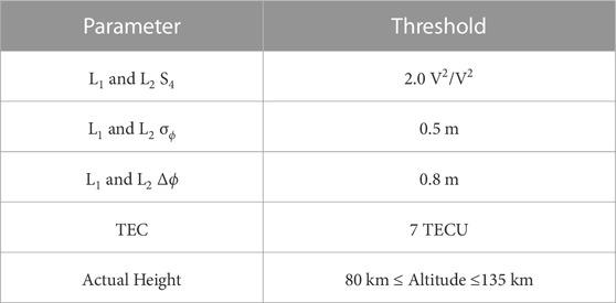
TABLE 2. Thresholds placed on GNSS-RO perturbation and scintillation parameters and E_s actual heights to remove outliers for quality control.

For foEs (Figure 3), L₁ and L₂ σ_ϕ show relatively strong correlations with ρ > 0.6. Linear fits also present larger slopes that reach an foEs of 6 MHz for maximum values of L₁ σ_ϕ, which is not reached for any other parameter. This supports the results of Emmons et al. (2022), which suggested that σ_ϕ is a better parameter than S₄ for characterizing stronger E_s layers.

The results and trends for fbEs are similar to foEs but with stronger correlations (Figure 4). This stronger correlation may be due to the more uniform nature of blanketing E_s layers compared to the patchy/cloudy layers (Reddy and Mukunda Rao, 1968). Previous GNSS-RO models of sporadic-E intensity have focused on fbEs instead of foEs for exactly this reason (Arras and Wickert, 2018; Gooch et al., 2020). However, there are fewer fbEs measurements, and not all sporadic-E layers are blanketing, which places a limitation on models using fbEs.

Unlike foEs, the foμEs estimates show the strongest correlations with S₄ (Figure 5). However, the correlations are weaker and there are many low foμEs values for large values of the RO parameter. This is most obvious for TEC, which shows a moderate correlation with foEs, but a weak correlation to foμEs along with a nearly flat linear fit (slope near zero). The collection of low foμEs points is likely due to uncertainties in the background E-region densities introduced by IRI in the foEs to foμEs conversion. These weaker correlations and linear fits highlight the practical challenges of using the metallic-ion parameters. While these metallic-ion parameters are certainly more appropriate for GNSS-RO measurements, the uncertainties introduced by using a model to estimate the background E-region can add unwanted errors to the dataset.

The fbμEs estimates show moderate correlations with S₄ and σ_ϕ (Figure 6). However, the correlations are weaker than for fbEs, likely due to the uncertainty added by the IRI estimates, as discussed for foμEs. All of the GNSS-RO scintillation and perturbation parameter correlations with ionosonde derived intensity parameters are statistically significant with p-values ≤0.01. Only the TEC correlation with foμEs provides a p-value of 0.01, while all others are less than 0.01.

3.3 Model development and feature importance

To select an appropriate model for predicting E_s intensities (fEs) using GNSS-RO perturbation and scintillation parameters, the Lazy Predict regression package implemented in Python (https://pypi.org/project/lazypredict/; accessed July 2023) was used to test a variety of models on this particular dataset. From Lazy Predict (results not shown), the top performing models for all intensity parameters were Epsilon Support Vector Regression (SVR) and Random Forest, as implemented through scikit-learn (Pedregosa et al., 2011). After applying and optimizing both the SVR and Random Forest models, the SVR model using a linear kernel showed the best overall performance in terms of R² and Mean Absolute Error (MAE), so this linear-SVR model was implemented as our primary E_s intensity model. The performance improvement using a linear kernel over nonlinear kernels is somewhat surprising given previous studies that found optimal fits to nonlinear forms, such as the Yu et al. (2020) S₄ to foEs formula: (foEs −1.2)² = 13.62 ×S_4,max.

In addition to the SVR model, a multiple linear regression model (MLR) is developed to provide a simplified approach for relatively easy implementation. Further, the two newer models are compared to previous GNSS-RO based fEs models from the literature. Specifically, the TEC technique described in Gooch et al. (2020) and the S₂ technique of Arras and Wickert (2018) were used as the baseline fEs models. It should be noted that the two baseline models were developed using fbEs, which may skew the results when comparing against foEs/foμEs/fbμEs.

A train–test split was implemented using data before 1 January 2015 for training and data after for testing. This results in a roughly 70%–30% split for training–testing. The total number of data points for each ionosonde intensity parameter is displayed in Table 3. Only the training data set is used for model development and tuning.

TABLE 3

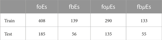
TABLE 3. The number of observations used for training and testing, split by ionosonde intensity parameter.

For model development, a Permutation Feature Importance (PFI) was calculated for each of the model features (GNSS-RO perturbation and scintillation parameters) and ionosonde intensity parameters. PFI shows the decrease in a metric from randomly shuffling the feature of interest. Here, we use a composite metric based on an equal weighting of MAE and R². The features with the largest decrease are generally the most important features in terms of model performance. As displayed in Figure 7, all ionosonde intensity models except fbEs show the L₁ S₄ as the most important feature, which supports the heavy reliance on amplitude scintillation in previous GNSS-RO-derived E_s intensity estimates [e.g., Arras and Wickert (2018); Yu et al. (2020)]. For fbEs, TEC is the most important parameter, which matches the results of Gooch et al. (2020).

FIGURE 7

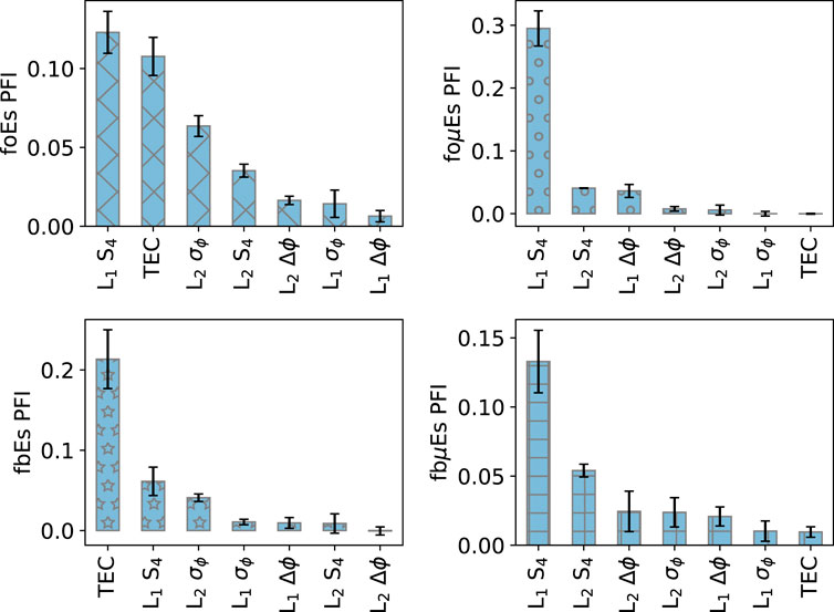
FIGURE 7. Permutation Feature Importance (PFI) for the GNSS-RO scintillation and perturbation parameters in a linear SVR model. The bars correspond to the mean decrease in the MAE–R² composite metric from randomly shuffling the feature of interest with 1,000 iterations, and the error bars correspond to the standard deviation.

The relative feature importance varies dramatically between the different ionosonde intensity parameters. For example, TEC is the most important for fbEs and is a close second to the L₁ S₄ for foEs, but it is the least important feature for foμEs and fbμEs. Generally, L₂ σ_ϕ is important to foEs and fbEs while L₂ S₄ is important for the metallic-ion (μ) models. Emmons et al. (2022) found σ_ϕ to provide valuable information to interpreting GNSS-RO scintillation observations due to the S₄ saturation that can occur for stronger layers (Stambovsky et al., 2021). This matches the PFI results for foEs and fbEs, but the phase perturbation Δϕ is more important than σ_ϕ for the metallic-ion parameters foμEs/fbμEs likely due to the uncertainties introduced by IRI estimates of the background E-region density.

Interestingly, the relative importance of the different features do not match the relative strength of the linear fit R² and Spearman ρ values displayed in Figures 3–6. For example, the strongest linear fit values for the GNSS-RO parameters to foEs (Figure 3) are from σ_ϕ, while L₁ S₄ and TEC are the most important features in the SVR model. This is likely due to differences between simple linear regression and SVR, which places different weights and penalties on the data (Smola and Schölkopf, 2004).

For the final SVR and MLR models, we use the top four most important features for each ionosonde intensity parameter to build the final model. Future studies can focus on reducing the number of input variables while maintaining performance, but here we use four parameters for each model for simplicity and consistency. The SVR ϵ and regularization (C) parameters were also tuned to optimize performance using the MAE–R² composite metric [a description of these SVR parameters can be found in Smola and Schölkopf (2004)]. The parameters were tuned using a 5-fold cross-validation search over a full grid of parameters, resulting in the values displayed in Table 4.

TABLE 4

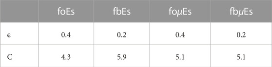
TABLE 4. The SVR ϵ and C parameters optimized for each ionosonde intensity parameter.

For reference, the MLR slopes and intercepts are displayed in Table 5 for each ionosonde intensity parameter. While four GNSS-RO perturbation and intensity parameters were used for each model, a couple of parameters have negative slopes, indicating that the number of input parameters can be fine-tuned in future studies to optimize and simplify the models. It must also be noted that the various GNSS-RO parameters are not independent, and the complex mapping from E_s characteristics to RO diffraction patterns is not fully understood. This mapping was explored in detail in Emmons et al. (2022), showing a linear relationship between L₁–S₄ and σ_ϕ for the majority of mid-latitude occultations, suggesting that a linear approach may be appropriate for most E_s measurements. The MLR approach implemented here assumes a simple linear relationship between the RO parameters and the E_s intensity, allowing contributions from both phase and amplitude perturbations. While future model optimization may be able to produce similar results using fewer features (input variables), here we use the same features as the SVR model following the feature importance results displayed in Figure 7.

TABLE 5

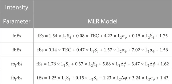
TABLE 5. GNSS-RO MLR intensity models for each ionosonde intensity parameter. The units and parameter calculation details are displayed in Table 1.

To quantify the statistical significance of the new MLR model, an F-test was performed on the training dataset testing against the null hypothesis that all model parameters are zero. The F-test produced a minimum F-statistic of 22 for the fbμEs model with an associated p-value of $<$ 0.001. All other models produced larger F-statistics and lower p-values, indicating a very high significance in the results which allows us to reject the null hypothesis and conclude that the model results are not due to randomness.

3.4 Model performance

GNSS-RO fEs estimates are displayed against the ionosonde intensity parameters in Figures 8–11. Linear fits and uncertainties are calculated using a bootstrapping approach from 10,000 samples with replacement (Gareth et al., 2013). The overall improvement in the MLR and SVR models is immediately obvious relative to the baseline S₂ and TEC approaches. Furthermore, the strong similarities between the MLR and linear-SVR approaches are apparent, with slight differences due to the weighting schemes and penalties for the two models.

FIGURE 8

FIGURE 8. GNSS-RO fEs estimates versus ionosonde foEs observations. Slope and intercept uncertainties are from the standard errors. Note the improved performance for the MLR and SVR models relative to the baseline S₂ and TEC models. The unfilled markers correspond to daytime measurements while the filled markers designate nighttime measurements.

FIGURE 9

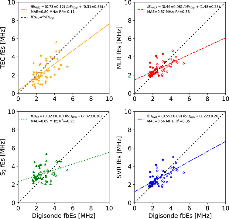
FIGURE 9. GNSS-RO fEs estimates versus ionosonde fbEs observations. The unfilled markers correspond to daytime measurements while the filled markers designate nighttime measurements. Note the relatively large slope for the TEC-based technique.

FIGURE 10

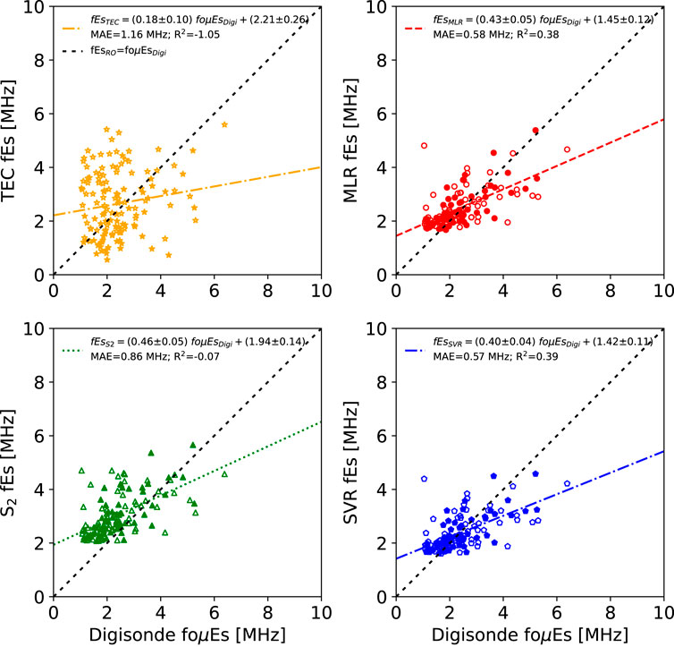
FIGURE 10. GNSS-RO fEs estimates versus ionosonde-based foμEs observations. The unfilled markers correspond to daytime measurements while the filled markers designate nighttime measurements. Note the nearly flat slope for the TEC-based technique and the weaker performance for the MLR and SVR models relative to Figure 8.

FIGURE 11

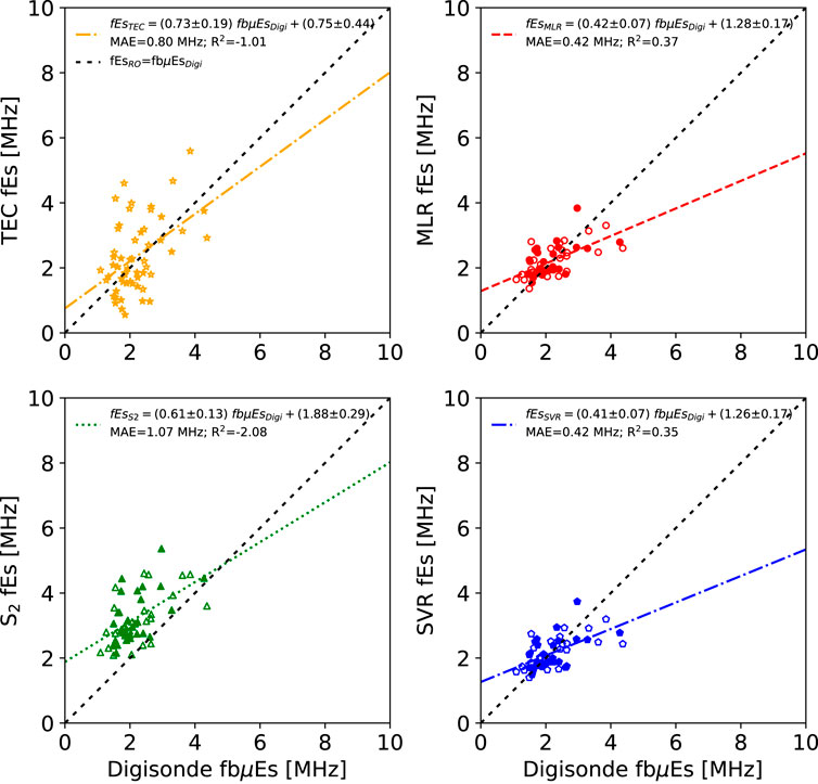
FIGURE 11. GNSS-RO fEs estimates versus ionosonde-based fbμEs observations. The unfilled markers correspond to daytime measurements while the filled markers designate nighttime measurements. Note the low MAE for the MLR and SVR models.

Predictions from the foEs models are displayed in Figure 8. The TEC technique generally underestimates, resulting in a negative R² value and an MAE of 0.9 MHz. Negative R² values indicate that the model predictions have a larger sum of squared residuals than a model that simply predicts the average of the observed data, which corresponds to R² = 0. In other words, the average of the squared residuals is larger than the variance in the observed data, which can indicate a bias in the model as observed here. The S₂ approach has a positive but weak R² with a low slope and a narrow spread of estimates, resulting in an MAE of 0.7 MHz.

Both the MLR and SVR approaches perform similarly, with moderate R² values and a low MAE of 0.5 MHz. It must be noted that this MAE is within the range of ARTIST-5 foEs error bounds [(−0.80, 0.35) MHz; Stankov et al. (2023)], indicating that some of the error may be the result of uncertainties from ARTIST-5 predictions. However, as observed in Figure 8, RO-based techniques systematically underestimate the strong E_s layer intensities, as demonstrated by the linear fit slopes of fEs_RO ≈ 0.5 foEs_Digi for the MLR and SVR models, resulting in foEs errors that cannot be explained by the uncertainties of ARTIST-5. However, this result is not surprising given the models’ reliance on S₄ which is known to saturate for stronger E_s layers (Stambovsky et al., 2021; Emmons et al., 2022). In addition, both models perform better for daytime measurements with slight overpredictions of weak nighttime intensities. The increased daytime performance is consistent with a recent study by Sobhkhiz-Miandehi et al. (2023), which found a stronger agreement between ionosonde and RO measurements during the day with low solar zenith angles.

Similar behavior is observed for the fbEs estimates (Figure 9), with a general improvement in the fEs estimates by the MLR and SVR models. Interestingly, all of the models perform slightly worse for fbEs than foEs, except for the TEC approach, which shows a slight improvement. This general decrease in performance for fbEs models may be due to the limited number of data points compared to foEs. However, the decrease in MLR and SVR performance is slight, with MAEs increasing from 0.5 to 0.6 MHz. As with foEs, both the MLR and SVR models perform better for daytime measurements.

The metallic-ion based foμEs results are displayed in Figure 10, which show similar performance for the fbEs estimates for all models except for TEC. TEC fEs estimates show a drastic decrease in performance with a nearly flat slope of fEs_RO ≈ 0.2 foEs_Digi. This poor performance of the TEC model is likely an artifact of the foEs to foμEs conversion that relies on IRI, which introduces an additional uncertainty into the estimates. The large collection of data points with low foμEs and a large spread of TEC values on the left side of the TEC figure is likely caused by overestimates of the background E-region densities, resulting in a cluster of small foμEs values. While this behavior is also observed in the other foμEs models, they are less severe resulting in slopes between 0.4 and 0.5 instead of the TEC slope of 0.2. Unlike foEs and fbEs, the MLR and SVR models for foμEs perform better for nighttime measurements, due to overestimates of the daytime background E-region densities used in the foEs to foμEs conversion.

The fbμEs estimates also show a bias towards lower fbμEs values due to overestimates of the background E-region densities (Figure 11). However, this bias is most obvious in the S₂ model, while the TEC model performs significantly better than the TEC foμEs model. The MLR and SVR models have the lowest MAE values of 0.4 MHz of all ionosonde intensity parameters, but the R² values and slopes are slightly lower than the foEs models. This low MAE is likely the result of lower intensities with a peak fbμEs of approximately 4 MHz, compared to the peak foEs magnitudes above 6 MHz.

4 Discussion

Several interesting results have emerged from this study. First, it appears that while the physical reasoning of the metallic-ion foμEs and fbμEs parameters is appropriate to quantify the EDP enhancement induced by E_s (Haldoupis, 2019), the practical implementation is challenging due to the reliance on E-region electron density predictions from models such as IRI. While it may seem more appropriate to use ionosonde-based electron density estimates for the conversion, this is also practically limited by the presence of sporadic-E which results in low confidence scores for the ARTIST ionogram inversion process (Galkin et al., 2013). Model errors can introduce additional uncertainty in foμEs and fbμEs, which appears to explain the elevated MAE and reduced R² in Figure 10 compared to Figure 8. While nighttime background E-region contributions to foEs and fbEs are negligible (see the points near the 1:1 line in Figure 2), many of the daytime density predictions appear to be overestimated, significantly affecting lower intensity layers (see the collection of foμEs points at the lower limit of 1 MHz in Figure 2) which results in poorer model performance for foμEs compared to foEs. Perhaps using alternative E-region models such as the rocket-based Faraday-International Reference Ionosphere [FIRI; (Friedrich and Torkar, 2001)] could improve the metallic-ion-based model performance. However, given the results of this study, it seems that comparing GNSS-RO estimates against ionosonde direct measurements of foEs and fbEs is the most practical approach at the moment to limit the overall uncertainties in the datasets.

A second interesting result is the strong correlations of the different ionosonde intensity parameters with respect to the phase scintillation parameter σ_ϕ (Figures 3–6). Many previous studies have used phase-based perturbations (Chu et al., 2014; Niu et al., 2019; Gooch et al., 2020) and amplitude scintillation (Wu et al., 2005; Arras and Wickert, 2018; Yu et al., 2019) to characterize sporadic-E, but few studies focus on σ_ϕ (Wu et al., 2005; Wu, 2006; Emmons et al., 2022). While the newly developed MLR and SVR models rely more heavily on S₄ (and TEC for fbEs), L₂ σ_ϕ was shown to be important for foEs and fbEs models. This relatively unexplored parameter for E_s should be examined in more detail in future studies.

Finally, while it is no surprise that the newly developed multiple linear regression (MLR) and support vector regression (SVR) models improved intensity estimates for each ionosonde parameter, the relatively low fEs_RO to fEs_Digi slopes of 0.5 show that these new models still struggle to predict intensities for stronger layers (Figures 8–11). The difficulty in predicting larger fEs values is due to the strong dependence of the models on S₄, which is known to saturate for strong layers (Stambovsky et al., 2021; Emmons et al., 2022). Future modeling efforts focusing on stronger E_s layers will likely find more benefit from phase-based σ_ϕ rather than amplitude-based S₄.

Perhaps the largest obstacle in the quest to develop accurate E_s intensity estimates from GNSS-RO observations is the variable nature of the spatial extent and orientation of sporadic-E. Given the cylindrical horizontal shape of the E_s layers with wide distributions in both horizontal extent (Cathey, 1969; Maeda and Heki, 2015) and vertical thickness (Zeng and Sokolovskiy, 2010), the GNSS-RO response for a given fEs can show drastic variations for different lengths and thicknesses [e.g., see discussion and simulations in Emmons et al. (2022)]. The geometry of the RO path through the E_s layer is also unknown, as the horizontal orientation (i.e., north-south or east-west) of the E_s layer cannot be determined solely from a single GNSS-RO observation. This orientation uncertainty can potentially be resolved by using multiple RO observations of a single E_s layer by combining line-of-sight (LOS) angles with amplitude and phase perturbations. The larger perturbations would correspond to longer signal paths through the E_s layer, which can be used to provide orientation and temporal dynamics similar to the ground-based TEC observations from Maeda and Heki (2015).

In addition, small-scale structures and turbulence caused by Kelvin-Helmholtz instabilities (Bernhardt, 2002; Hysell et al., 2016) can create significant changes in GNSS-RO observations [also discussed in Emmons et al. (2022)]. Finally, a recent comparison of ionosonde with RO observations found the best agreement during the day of local summer and also noted that certain ionosonde sites systematically showed stronger agreement with RO E_s observations (Sobhkhiz-Miandehi et al., 2023). This site-to-site and temporal variation is the result of site-dependent ionosonde hardware, background ionosphere fluctuations, and perhaps a geographic and temporal dependence of E_s spatial characteristics and small-scale structures, which should be examined in more detail in future studies.

These various factors result in an inherent uncertainty to the fEs intensity estimates from GNSS-RO observations, which may be difficult to resolve without the help of additional sensors or multiple GNSS-RO observations with sufficient spatial resolution. Luckily, the current global RO spatial and temporal measurement density allows for high resolution analyses, as recently demonstrated for sporadic-E (Arras et al., 2022; Hodos et al., 2022), the lower ionosphere (Wu et al., 2022), and the F-region ionosphere (Swarnalingam et al., 2023; Wu et al., 2023).

5 Conclusion

Two new models of sporadic-E intensity from GNSS-RO observations were developed and compared with ionosonde observations. The new models were developed using L₁ and L₂ GNSS-RO measurements through sporadic-E layers within 50 km and 30 min of ionosonde observations, providing concurrent measurements of GNSS-RO phase and amplitude perturbations along with ionosonde intensity parameters foEs and fbEs. Metallic-ion-based foμEs and fbμEs intensity parameters were also calculated using IRI-2016 to remove the background E-region ion density from the ionosonde foEs and fbEs observations, providing estimates of the metallic-ion density perturbations to the slowly varying background ionosphere. The key results are summarized below:

• Multiple linear regression (MLR) and support vector regression (SVR) models demonstrate a drastic increase in performance over the baseline TEC and S₂ approaches. This increase in performance is due to the inclusion of both L₁ and L₂ phase and amplitude perturbation and scintillation indices, instead of only relying on phase (TEC) or amplitude (S₂).

• While the new models showed better performance overall, they struggled to predict the strong E_s layer intensities, likely due to a heavy reliance on S₄ which is known to saturate.

• Comparisons of the various ionosonde intensity parameters (foEs, fbEs, foμEs, and fbμEs) with GNSS-RO perturbation and scintillation parameters showed a strong correlation with phase scintillation σ_ϕ. This σ_ϕ parameter has not been widely implemented in GNSS-RO monitoring of sporadic-E, and here we recommend a closer inspection of the usefulness in future studies.

• Finally, while the metallic-ion-based foμEs and fbμEs parameters are the most physically ideal parameters to compare against GNSS-RO observations, the reliance on modeled background E-region densities makes the practical implementation difficult. The uncertainty introduced by the ionospheric model (here we used IRI-2016) can outweigh the original uncertainties from direct foEs and fbEs measurements. Given the large number of foEs observations relative to fbEs, we recommend comparing GNSS-RO with ionosonde-derived foEs for future development.

Implementation of either the MLR or SVR models outlined here can help improve GNSS-RO-based intensity estimates for global climatologies, morphologies, and radio operations.

Data availability statement

The raw data supporting the conclusion of this article will be made available by the authors, without undue reservation.

Author contributions

DE: Conceptualization, Formal Analysis, Investigation, Writing–original draft, Writing–review and editing. DW: Conceptualization, Formal Analysis, Investigation, Writing–original draft. NS: Conceptualization, Formal Analysis, Investigation, Writing–original draft. AA: Conceptualization, Formal Analysis, Investigation, Writing–original draft. JE: Conceptualization, Formal Analysis, Investigation, Writing–original draft. KF: Conceptualization, Formal Analysis, Investigation, Writing–original draft. KO: Conceptualization, Formal Analysis, Investigation, Writing–original draft.

Funding

The author(s) declare financial support was received for the research, authorship, and/or publication of this article. This research was funded by the Air Force Office of Scientific Research (AFOSR/RTB1), and NASA’s Living With Star and Sun-Climate research funds to the Goddard Space Flight Center (GSFC) under WBS 936723.02.01.12.48.

Acknowledgments

We would like to thank the Digital Ionogram Database (DIDBase) and the COSMIC Data Analysis and Archive Center (CDAAC) for the use of their data.

Conflict of interest

The authors declare that the research was conducted in the absence of any commercial or financial relationships that could be construed as a potential conflict of interest.

Publisher’s note

All claims expressed in this article are solely those of the authors and do not necessarily represent those of their affiliated organizations, or those of the publisher, the editors and the reviewers. Any product that may be evaluated in this article, or claim that may be made by its manufacturer, is not guaranteed or endorsed by the publisher.

Author disclaimer

The views, opinions, and/or findings expressed are those of the author and should not be interpreted as representing the official views or policies of the Department of Defense or the U.S. Government.

References

Ahmad, B. (1999). Accuracy and resolution of atmospheric profiles obtained from radio occultation measurements. Stanford University.

Google Scholar

Arras, C., Resende, L. C. A., Kepkar, A., Senevirathna, G., and Wickert, J. (2022). Sporadic E layer characteristics at equatorial latitudes as observed by GNSS radio occultation measurements. Earth, Planets Space 74, 163. doi:10.1186/s40623-022-01718-y

CrossRef Full Text | Google Scholar

Arras, C., and Wickert, J. (2018). Estimation of ionospheric sporadic E intensities from GPS radio occultation measurements. J. Atmos. Solar-Terrestrial Phys. 171, 60–63. doi:10.1016/j.jastp.2017.08.006

CrossRef Full Text | Google Scholar

Bernhardt, P. A. (2002). The modulation of sporadic-E layers by Kelvin–Helmholtz billows in the neutral atmosphere. J. Atmos. solar-terrestrial Phys. 64, 1487–1504. doi:10.1016/s1364-6826(02)00086-x

CrossRef Full Text | Google Scholar

Bilitza, D., Altadill, D., Truhlik, V., Shubin, V., Galkin, I., Reinisch, B., et al. (2017). International Reference Ionosphere 2016: from ionospheric climate to real-time weather predictions. Space weather. 15, 418–429. doi:10.1002/2016sw001593

CrossRef Full Text | Google Scholar

Briggs, B., and Parkin, I. (1963). On the variation of radio star and satellite scintillations with zenith angle. J. Atmos. Terr. Phys. 25, 339–366. doi:10.1016/0021-9169(63)90150-8

CrossRef Full Text | Google Scholar

Carmona, R. A., Nava, O. A., Dao, E. V., and Emmons, D. J. (2022). A comparison of sporadic-E occurrence rates using GPS radio occultation and ionosonde measurements. Remote Sens. 14, 581. doi:10.3390/rs14030581

CrossRef Full Text | Google Scholar

Cathey, E. H. (1969). Some midlatitude sporadic-E results from the Explorer 20 satellite. J. Geophys. Res. 74, 2240–2247. doi:10.1029/ja074i009p02240

CrossRef Full Text | Google Scholar

Chu, Y.-H., Wang, C., Wu, K., Chen, K., Tzeng, K., Su, C.-L., et al. (2014). Morphology of sporadic E layer retrieved from COSMIC GPS radio occultation measurements: wind shear theory examination. J. Geophys. Res. Space Phys. 119, 2117–2136. doi:10.1002/2013ja019437

CrossRef Full Text | Google Scholar

Emmons, D. J., Wu, D. L., and Swarnalingam, N. (2022). A statistical analysis of sporadic-E characteristics associated with GNSS radio occultation phase and amplitude scintillations. Atmosphere, 2098.

CrossRef Full Text | Google Scholar

Fabrizio, G. A. (2013). High frequency over-the-horizon radar: fundamental principles, signal processing, and practical applications. McGraw-Hill Education.

Google Scholar

Friedrich, M., and Torkar, K. (2001). FIRI: a semiempirical model of the lower ionosphere. J. Geophys. Res. Space Phys. 106, 21409–21418. doi:10.1029/2001ja900070

CrossRef Full Text | Google Scholar

Galkin, I., Reinisch, B. W., Huang, X., and Khmyrov, G. M. (2013). Confidence score of ARTIST-5 ionogram autoscaling. Ionosonde Netw. Advis. Group (INAG) Bull. 1–7.

PubMed Abstract | Google Scholar

Galkin, I. A., and Reinisch, B. W. (2008). The new ARTIST 5 for all Digisondes. Ionosonde Netw. Advis. Group Bull. 69, 1–8.

Google Scholar

Gareth, J., Daniela, W., Trevor, H., and Robert, T. (2013). An introduction to statistical learning: with applications in R (Spinger).

Google Scholar

Gooch, J. Y., Colman, J. J., Nava, O. A., and Emmons, D. J. (2020). Global ionosonde and GPS radio occultation sporadic-E intensity and height comparison. J. Atmos. Solar-Terrestrial Phys. 199, 105200. doi:10.1016/j.jastp.2020.105200

CrossRef Full Text | Google Scholar

Haldoupis, C. (2011). A tutorial review on sporadic E layers. Aeronomy Earth’s Atmos. Ionos., 381–394. doi:10.1007/978-94-007-0326-1_29

CrossRef Full Text | Google Scholar

Haldoupis, C. (2019). An improved ionosonde-based parameter to assess sporadic E layer intensities: a simple idea and an algorithm. J. Geophys. Res. Space Phys. 124, 2127–2134. doi:10.1029/2018ja026441

CrossRef Full Text | Google Scholar

Hocke, K., Igarashi, K., Nakamura, M., Wilkinson, P., Wu, J., Pavelyev, A., et al. (2001). Global sounding of sporadic E layers by the GPS/MET radio occultation experiment. J. Atmos. Solar-Terrestrial Phys. 63, 1973–1980. doi:10.1016/s1364-6826(01)00063-3

CrossRef Full Text | Google Scholar

Hodos, T. J., Nava, O. A., Dao, E. V., and Emmons, D. J. (2022). Global sporadic-E occurrence rate climatology using GPS radio occultation and ionosonde data. JGR Space Phys. 127. doi:10.1029/2022ja030795

CrossRef Full Text | Google Scholar

Hysell, D. L., Larsen, M., and Sulzer, M. (2016). Observational evidence for new instabilities in the midlatitude <i&amp;gt;E&amp;lt;/i&amp;gt; and <i&amp;gt;F&amp;lt;/i&amp;gt; region. Ann. Geophys. 34, 927–941. doi:10.5194/angeo-34-927-2016

CrossRef Full Text | Google Scholar

Luo, J., Liu, H., and Xu, X. (2021). Sporadic E morphology based on COSMIC radio occultation data and its relationship with wind shear theory. Earth, Planets Space 73, 212–217. doi:10.1186/s40623-021-01550-w

CrossRef Full Text | Google Scholar

Maeda, J., and Heki, K. (2015). Morphology and dynamics of daytime mid-latitude sporadic-E patches revealed by GPS total electron content observations in Japan. Earth, Planets Space 67, 89–9. doi:10.1186/s40623-015-0257-4

CrossRef Full Text | Google Scholar

Mathews, J. (1998). Sporadic E: current views and recent progress. J. Atmos. solar-terrestrial Phys. 60, 413–435. doi:10.1016/s1364-6826(97)00043-6

CrossRef Full Text | Google Scholar

McNamara, L. F. (1991). The ionosphere: communications, surveillance, and direction finding. Malabar, Florida, United States: Krieger publishing company.

Google Scholar

Merriman, D., Nava, O., Dao, E., and Emmons, D. (2021). Comparison of seasonal foEs and fbEs occurrence rates derived from global Digisonde measurements. Submitted to MDPI Atmosphere.

CrossRef Full Text | Google Scholar

Niu, J., Weng, L., Meng, X., and Fang, H. (2019). Morphology of ionospheric sporadic E layer intensity based on COSMIC occultation data in the midlatitude and low-latitude regions. J. Geophys. Res. Space Phys. 124, 4796–4808. doi:10.1029/2019ja026828

CrossRef Full Text | Google Scholar

Pedregosa, F., Varoquaux, G., Gramfort, A., Michel, V., Thirion, B., Grisel, O., et al. (2011). Scikit-learn: machine learning in Python. J. Mach. Learn. Res. 12, 2825–2830.

Google Scholar

Reddy, C., and Mukunda Rao, M. (1968). On the physical significance of the Es parameters fbEs, fEs, and foEs. J. Geophys. Res. 73, 215–224. doi:10.1029/ja073i001p00215

CrossRef Full Text | Google Scholar

Savitzky, A., and Golay, M. J. (1964). Smoothing and differentiation of data by simplified least squares procedures. Anal. Chem. 36, 1627–1639. doi:10.1021/ac60214a047

CrossRef Full Text | Google Scholar

Shinagawa, H., Tao, C., Jin, H., Miyoshi, Y., and Fujiwara, H. (2021). Numerical prediction of sporadic E layer occurrence using GAIA. earth, planets space 73, 28–18. doi:10.1186/s40623-020-01330-y

CrossRef Full Text | Google Scholar

Singleton, D. (1970). Saturation and focusing effects in radio-star and satellite scintillations. J. Atmos. Terr. Phys. 32, 187–208. doi:10.1016/0021-9169(70)90191-1

CrossRef Full Text | Google Scholar

Smith, E. K. (1957). Worldwide occurrence of sporadic E., 582. Washington DC, United States: US Department of Commerce, National Bureau of Standards.

Google Scholar

Smola, A. J., and Schölkopf, B. (2004). A tutorial on support vector regression. Statistics Comput. 14, 199–222. doi:10.1023/b:stco.0000035301.49549.88

CrossRef Full Text | Google Scholar

Sobhkhiz-Miandehi, S., Yamazaki, Y., Arras, C., and Themens, D. (2023). A comparison of FORMOSAT-3/COSMIC radio occultation and ionosonde measurements in sporadic E detection over mid and low latitude regions. Front. Astronomy Space Sci. 10, 1198071. doi:10.3389/fspas.2023.1198071

CrossRef Full Text | Google Scholar

Stambovsky, D. W., Colman, J. J., Nava, O. A., and Emmons, D. J. (2021). Simulation of GPS radio occultation signals through Sporadic-E using the multiple phase screen method. J. Atmos. Solar-Terrestrial Phys. 214, 105538. doi:10.1016/j.jastp.2021.105538

CrossRef Full Text | Google Scholar

Stankov, S., Verhulst, T., and Sapundjiev, D. (2023). Automatic ionospheric weather monitoring with DPS-4D ionosonde and ARTIST-5 autoscaler: System performance at a mid-latitude observatory. Radio Sci. 58, 1–20. doi:10.1029/2022rs007628

CrossRef Full Text | Google Scholar

Swarnalingam, N., Wu, D. L., Emmons, D. J., and Gardiner-Garden, R. (2023). Optimal estimation inversion of ionospheric electron density from GNSS-POD limb measurements: Part II-validation and comparison using NmF2 and hmF2. Remote Sens. 15, 4048. doi:10.3390/rs15164048

CrossRef Full Text | Google Scholar

Syndergaard, S. (2006). COSMIC S4 data. Boulder, CO, USA: UCAR/CDAAC.

Google Scholar

Tsai, L.-C., Su, S.-Y., Liu, C.-H., Schuh, H., Wickert, J., and Alizadeh, M. M. (2018). Global morphology of ionospheric sporadic E layer from the FormoSat-3/COSMIC GPS radio occultation experiment. GPS Solutions 22, 118. doi:10.1007/s10291-018-0782-2

CrossRef Full Text | Google Scholar

Whitehead, J. (1989). Recent work on mid-latitude and equatorial sporadic-E. J. Atmos. Terr. Phys. 51, 401–424. doi:10.1016/0021-9169(89)90122-0

CrossRef Full Text | Google Scholar

Wu, D. L. (2006). Small-scale fluctuations and scintillations in high-resolution GPS/CHAMP SNR and phase data. J. Atmos. solar-terrestrial Phys. 68, 999–1017. doi:10.1016/j.jastp.2006.01.006

CrossRef Full Text | Google Scholar

Wu, D. L., Ao, C. O., Hajj, G. A., de La Torre Juarez, M., and Mannucci, A. J. (2005). Sporadic E morphology from GPS-CHAMP radio occultation. J. Geophys. Res. Space Phys. 110. doi:10.1029/2004ja010701

CrossRef Full Text | Google Scholar

Wu, D. L., Emmons, D. J., and Swarnalingam, N. (2022). Global GNSS-RO electron density in the lower ionosphere. Remote Sens. 14, 1577. doi:10.3390/rs14071577

CrossRef Full Text | Google Scholar

Wu, D. L., Swarnalingam, N., Salinas, C. C. J. H., Emmons, D. J., Summers, T. C., and Gardiner-Garden, R. (2023). Optimal estimation inversion of ionospheric electron density from GNSS-POD limb measurements: Part I-algorithm and morphology. Remote Sens. 15, 3245. doi:10.3390/rs15133245

CrossRef Full Text | Google Scholar

Yeh, W.-H., Liu, J.-Y., Huang, C.-Y., and Chen, S.-P. (2014). Explanation of the sporadic-E layer formation by comparing FORMOSAT-3/COSMIC data with meteor and wind shear information. J. Geophys. Res. Atmos. 119, 4568–4579. doi:10.1002/2013jd020798

CrossRef Full Text | Google Scholar

Yu, B., Scott, C. J., Xue, X., Yue, X., and Dou, X. (2020). Derivation of global ionospheric Sporadic E critical frequency (fo Es) data from the amplitude variations in GPS/GNSS radio occultations. R. Soc. open Sci. 7, 200320. doi:10.1098/rsos.200320

PubMed Abstract | CrossRef Full Text | Google Scholar

Yu, B., Xue, X., Scott, C. J., Yue, X., and Dou, X. (2022). An empirical model of the ionospheric sporadic E layer based on GNSS radio occultation data. Space weather. 20, e2022SW003113. doi:10.1029/2022sw003113

CrossRef Full Text | Google Scholar

Yu, B., Xue, X., Yue, X., Yang, C., Yu, C., Dou, X., et al. (2019). The global climatology of the intensity of the ionospheric sporadic <i&amp;gt;E&amp;lt;/i&amp;gt; layer. Atmos. Chem. Phys. 19, 4139–4151. doi:10.5194/acp-19-4139-2019

CrossRef Full Text | Google Scholar

Yue, X., Schreiner, W. S., Pedatella, N. M., and Kuo, Y.-H. (2016). Characterizing GPS radio occultation loss of lock due to ionospheric weather. Space weather. 14, 285–299. doi:10.1002/2015sw001340

CrossRef Full Text | Google Scholar

Zeng, Z., and Sokolovskiy, S. (2010). Effect of sporadic E clouds on GPS radio occultation signals. Geophys. Res. Lett. 37. doi:10.1029/2010GL044561

CrossRef Full Text | Google Scholar