Observations and simulations of large-scale traveling ionospheric disturbances during the January 14-15, 2022 geomagnetic storm

Using the total electron content (TEC) observations from GPS, and simulations from the Thermosphere Ionosphere Electrodynamic General Circulation Model (TIEGCM), this work investigates the large-scale traveling ionospheric disturbances (LSTIDs) and the possible involved drivers during the geomagnetic storm on January 14-15, 2022. Based on the term analysis of O⁺ continuity equation in TIEGCM, it is found that the traveling atmospheric disturbances in equatorward winds are responsible for the LSTIDs, with minor contributions from plasma drifts owing to the prompt penetration electric field. A strong interhemispheric asymmetry of the LSTIDs is observed, which might be attributed to both the equatorward wind disturbances and background plasma. The stronger wind (plasma) disturbances occurs in the winter hemisphere than that in the summer hemisphere. The maximum magnitude of LSTIDs in electron density disturbances occurs at ∼250 and ∼270 km in the northern and southern hemispheres, respectively, owing to both the thermospheric equatorward winds and background plasma. An interesting phenomenon that tail-like LSTIDs occur at the dip equator and low latitudes might be related to the eruption of the Tonga volcano, but it is not well reproduced in TIEGCM that deserves further exploration in a future study.

1 Introduction

During the disturbance periods, the interaction between the interplanetary magnetic field (IMF) carried by the solar wind and the geomagnetic field could lead to the energy and momentum deposition from the solar wind to the Earth’s upper thermosphere (e.g., Dungey, 1961). A large amount of energy and momentum deposition triggers disturbances in the thermo-sphere, traveling to middle and low latitudes from the source region. The thermospheric wind perturbations associated with the generated traveling atmospheric disturbances (TADs) could push the ionospheric plasma upward or downward along the geomagnetic field lines, causing the enhancement or depletion in plasma, referred to as large-scale traveling ionospheric disturbances (TIDs). TADs/TIDs appear as wave-like perturbations in thermospheric/ionospheric observations, i.e., thermospheric meridional winds and density, ionospheric plasma. Over the past decades, a large variety of TIDs has been observed in a series of studies (e.g., Munro, 1958; Hocke et al., 1996; Balthazor et al., 1997; Shiokawa et al., 2007; 2013; MacDougall and Jayachandran, 2011; Yin et al., 2019; Zhang K et al., 2019; Zhang SR et al., 2019; Nishimura et al., 2020), which is a hot topic in the ionospheric research.

Based on the wavelength, phase speed, and period, TIDs could be categorized as large-scale and medium-scale (Bruinsma et al., 2009; Shiokawa et al., 2013). The large-scale TIDs (LSTIDs) have a period longer than 60 min, a horizontal velocity of 400–1,000 m/s, and a wavelength larger than 1,000 km, while the medium-scale TIDs have a period ranging from 15 min to 1 h, a horizontal velocity of 250–1,000 m/s and a wavelength of hundreds of kilometers (Afraimovich et al., 2000; Zhang SR et al., 2019). Previous studies have demonstrated that LSTIDs in the upper thermosphere could be generated by the geomagnetic activity (i.e., geomagnetic storm, and substorm) (Pi et al., 2000; Shiokawa et al., 1999; 2003; 2007; Afraimovich et al., 2008; Lei et al., 2008; Nicolls et al., 2012; Borries et al., 2016; Cherniak et al., 2018; Katamzi-Joseph et al., 2019; Zhang SR et al., 2019; Jonah et al., 2020).

In the literature, LSTIDs have been observed at high latitudes (Pi et al., 2000; Shiokawa et al., 2003; Nicolls et al., 2012). Using Fabry-Perot interferometer (FPI) observed neutral winds and incoherent scatter radar measured plasma drift at high latitudes in October 1992 for ∼36 h, Pi et al. (2000) reported outstanding evidence for TADs and LSTIDs generated by the aurora heating effects. Utilizing a series of measurements at high latitudes, including neutral winds from FPI and TEC from GPS, Shiokawa et al. (2003) found prominent LSTIDs during a major storm event with a minimum DST index of −358 nT on 31 March 2001. A turning of the thermospheric meridional winds from equatorward of 94 m/s to poleward of 44 m/s was observed, indicating an intense poleward wind in the thermosphere during the LSTIDs. The generation of poleward wind in the auroral zone could be associated with an intense substorm. Analyzing the FPI-measured thermospheric wind for atmospheric gravity waves (AGWs) over Alaska on January 9-10, 2010, Nicolls et al. (2012) reported an event of AGWs with a period of 32.7 ± 0.3 min, a horizontal wavelength of 1,094 ± 408 km, the phase speed of 560 ± 210 m/s, propagation azimuth of 33.5 ± 15.8° east-of-north, which was associated with enhanced auroral activity and the potential sources might be Joule heating, Lorentz force, and body forcing of horizontal winds due to auroral activity, etc.

Apart from high-latitude LSTIDs cases, in recent decades, a large number of studies have been performed to investigate the LSTIDs at middle and low latitudes (e.g., Shiokawa et al., 2002; Afraimovich et al., 2008; Lei et al., 2008; Jonah et al., 2020; Nishimura et al., 2020). Using a comprehensive TEC observation from GPS and simulation from the Sheffield University Plasmasphere-Ionosphere Model (SUPIM), Shiokawa et al. (2002) investigated a prominent LSTIDs detected at 23-24 LT (14-15 UT) during the magnetic storm on 15 September 1999, in Japan (16°–37° magnetic latitudes, MLat). The nighttime LSTIDs might be generated by the enhancement of poleward neutral winds which propagates equatorward. The SUPIM results suggested that the equatorward movement of poleward wind pulse was linked to the auroral energy input. Afraimovich et al. (2008) compared the intensity of LSTIDs with the local electron density disturbances during the magnetic storm on October 29–31, 2003, and November 7–11, 2004. They found that LSTIDs in TEC were dominated by the auroral energy, and the TEC variations were mainly attributed to the electron density disturbances at F2-layer. A numerical simulation from the coupled magneto-sphere-ionosphere model (CMIT) was performed and TEC data from GPS in Japan were analyzed to explore prominent northward LSTIDs and two southward LSTIDs events during the magnetic storm on 15 December 2006 (Lei et al., 2008). In their results, the northward LSTIDs were generated in the southern hemisphere which propagated into the northern hemisphere, however, two southward LSTIDs were not well captured in the model. A series of LSTIDs in ionospheric TEC perturbations were generated because of the intense magnetic storm on 17 March 2015 (Borries et al., 2016), which was induced by the Joule heating in the auroral region, Lorentz force from the perturbed electric fields, and a minor particle precipitation effect. The origin, occurrence, and propagation of LSTIDs over the European on December 19–21, 2015 were investigated in Cherniak and Zakharenkova (2018). Two major sources of the LSTIDs, the quiet-time solar terminator passage, and disturbed-time auroral activity have been reported. Using ground- and space-based measurements (i.e., Global Navigation Satellite System receivers, and Swarm satellites) and TIEGCM simulations during two magnetic storm periods, Jonah et al. (2020) found that the meridional winds (background ionospheric plasma) played important roles in the propagation (amplitude) of LSTIDs at middle and low latitudes. Smaller electron density was correlated with the smaller amplitude of LSTIDs, and vice versa.

Recently, a moderate geomagnetic storm occurs on January 14-15, 2022. Furthermore, a huge geohazard event of the Tonga volcano eruption [−20.5° geographic latitudes (GLat), −174.5° geographic longitudes (GLon)] has great effects on the ionosphere-thermosphere coupled system. This might complicate the ionospheric plasma responses. In this work, the TEC data from GPS, and numerical simulations from TIEGCM are used to investigate the ionospheric plasma responses during the moderate geomagnetic storm, which could contribute to the understanding of the coupling between high- and low-latitudes, between ionosphere and thermosphere. In the rest of this article, Section 2 introduces the GPS data and the model; Section 3 gives the results of LSTIDs and data-model comparison; Section 4 is the discussion about potential physical mechanisms; Section 5 summaries the results of this work.

2 Data and model

The GPS TEC dataset is obtained from the International Global Navigation Satellite System Service (IGS) Working Group, which is created in 1998 (Hernández-Pajares et al., 2009; Panda et al., 2022). The individual TEC maps are developed by eight Ionospheric Associate Analysis Centers (IAACs) under IGS. For example, the University of Bern (CODE, Switzerland), the European Space Agency (ESA, Germany), the Jet Propulsion Laboratory (JPL, America), and the University Politechnical Catalonia (UPC, Spain). The TEC data from IGS is the weighted mean of the eight analysis centers. The resolution of GPS TEC data in CDF format is 15 min, 1 and 2 h. A large amount of daily TEC files since 15 January 1998, is stored in IGS. In this work, TEC data with a resolution of 15 min on January 9-16, 2022 is used to explore the ionospheric disturbances during geomagnetic activity periods. The data could be downloaded from the link: https://cdaweb.gsfc.nasa.gov/pub/data/gps/tec15min_igs/2022/.

The Thermosphere Ionosphere Electrodynamic General Circulation Model (TIEGCM) is a three-dimensional time-dependent model of the coupled ionosphere-thermosphere system. It was developed at the High Altitude Observatory at the National Center for Atmospheric Research (NCAR/HAO). The driver of TIEGCM includes the high-latitude electric field from Heelis or Weimer models (Heelis et al., 1982; Weimer, 2005), the solar extreme ultraviolet and ultraviolet spectral fluxes that were parameterized by the F_10.7 index (Richards et al., 1994), the lower atmospheric migrating and non-migrating diurnal and semi-diurnal tides generated from the Global Scale Wave Model (GSWM) (Hagan and Forbes, 2002; 2003), or tides derived from the observations from the Sounding of the Atmosphere using Broadband Emission Radiometry and TIDI (Zhang et al., 2018; Wu et al., 2019). The horizontal resolution is 2.5° GLat × 2.5° GLon. TIEGCM has a total of 57 pressure levels in the vertical direction, with the lower and upper boundary of 97 km and ∼700 km (depending on the solar activity), respectively. In this study, the migrating and non-migrating tides from GSWM were specified at the lower boundary and the electric field from the Weimer model was imposed at high latitudes.

3 Results

3.1 Geomagnetic conditions

Figure 1A depicts the temporal variations of IMF Bz during the magnetic storm on January 14–16, 2022. It is found that IMF Bz is northward at 00–12 UT on January 14, with a maximum magnitude of 8.3 nT. At ∼12 UT on January 14, the northward IMF Bz starts to turn southward. The southward turning of IMF Bz arrives at its minimum value of −16.8 nT at 23 UT. Then, the strong southward IMF Bz quickly turns northward for a magnitude of ∼10 nT in 30 min. After that, the temporal variations of IMF Bz oscillate around 0 nT, with an absolute maximum magnitude of ∼8 nT. Figure 1B shows the temporal variations of Dst index on January 14–16, 2022. Based on the Dst index, the magnetic storm can be characterized by three phases, that is, initial, main, and recovery phases. During the initial phase of 08–12 UT on January 14, the Dst index is enhanced from 2 nT to 14 nT. During the main phase of 12–23 UT, the Dst index is significantly decreased to −91 nT. Then, during the recovery phase, the Dst index gets smoothly recovery to ∼−20 nT.

FIGURE 1

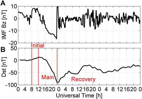
FIGURE 1. The temporal variations of IMF Bz (A) and Dst index (B) on January 14–16, 2022. The text of “Initial,” “Main” and “Recovery” in the bottom panel are the initial, main, and recovery phases of the magnetic storm, respectively.

3.2 Data-model comparison

Figures 2A, B show the geomagnetic latitude and UT variations of TEC observed from GPS and modeled by TIEGCM at −174.5° geographic longitude (GLon) on January 14–16, 2022. Note here that Tonga volcanic eruption occurs at −174.5° GLon. The data be-fore 14 UT on January 14 is not shown here, because the Dst index in Figure 1B starts to decrease to the negative peak at around 14 UT. The prominent feature of TEC is the strong equatorial ionization anomaly (EIA), which has been reported in a series of previous studies (e.g., Lin et al., 2005; Rajesh et al., 2021). During quiet time, EIA is the region between ±10° and ±15° magnetic latitude (MLat) across the magnetic equator (center) (e.g., Panda et al., 2018; Rajesh et al., 2021; Ogwala et al., 2022). As shown in Figure 2A, during the disturbed time, EIA in both hemispheres expands to higher latitudes, even to middle and high latitudes. The poleward edge could be seen at around ±60° MLat and 00 UT/12 LT on January 15. The maximum amplitude of TEC in the EIA region could reach ∼50 TECU at ±15° MLat and 00 UT/12 LT on January 15. At the dip equator, TEC is much weaker, with a value of ∼30 TECU, than that in the EIA region. These are the well-known two peaks of EIA (Lin et al., 2005). At the pre-dawn sector of 14–18 UT/02–06 LT on January 14, the GPS-observed TEC has an average value of ∼10 TECU, and the significant EIA has not been developed. With the onset of sunrise, the EIA begins to develop, and the maximum EIA occurs at around noon of 00–02 UT/12–14 LT on January 15. After the sunset of 08 UT/20 LT on January 15, the significant EIA disappears. During the daytime from 18 UT on January 15 to 08 UT on January 16, a similar prominent structure can be seen. An interesting phenomenon is found when the Tonga volcano eruption occurs, as indicated by the black star. A northward penetration of LSTID can be found at the post-dusk sector of 04–12 UT on January 15 after the eruption of Tonga volcano (black star), which seems like a tail-like structure following the EIA and deserves to explore. This tail-like structure disappears on January 16.

FIGURE 2

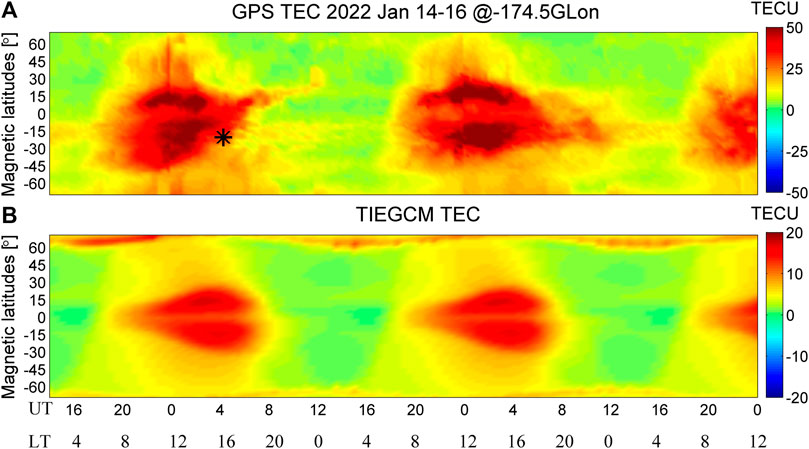
FIGURE 2. The geomagnetic latitude and UT variations of GPS observed TEC (A) and TIEGCM modeled TEC (B) at −174.5° GLon on January 14–16, 2022. TEC is given in TECU. The black star in Figure 2A is the time and location of the Tonga volcano eruption.

In Figure 2B, TIEGCM-modeled TEC also has a prominent character of EIA during daytime. A comparison between Figures 2A, B shows that the large-scale structure of TEC is similar to those two. The modeled EIA also expands to middle latitudes of ∼±60° MLat in both hemispheres, and the peaks of TEC also occur at around 02 UT/14 LT with a magnitude of ∼30 TECU. Compared to GPS-observed TEC, TEC in TIEGCM seems to be underestimated, which has been reported before (Shiokawa et al., 2007; Perlongo and Ridley, 2018) and might be attributed to the following potential reasons. For example, first, Joule heating tends to be underestimated in most large-scale models including TIEGCM due to the inability to capture small-scale features (Shiokawa et al., 2007). Second, the supply of O⁺ ions from the plasmasphere is underestimated in TIEGCM (Shiokawa et al., 2007). Third, the neutral winds are also underestimated in TIEGCM, as reported in previous studies (Perlongo and Ridley, 2018; Zhang et al., 2018). Fourth, the high-latitude electric field used in TIEGCM is an empirical model, which predicts only the state of plasma convection at high latitudes for a given 3-hourly Kp index or 1-min IMF, whereas the real high-latitude ion convection is much more complicated (Zhang et al., 2021). However, the large-scale structures of modeled TEC are similar to that of observed TEC, and a large degree of similarity between TIEGCM simulations and space-based/ground-based observations has been achieved in previous studies (Wang et al., 2012; Perlongo et al., 2018; Zhang et al., 2018; 2021). In summary, the reliability and stability of TIEGCM have been confirmed. Thus, it can be used to explore the ionospheric responses during the disturbed time in this work.

Representing the data-model comparison of the absolute vertical TEC, the ionospheric disturbances in TEC at −174.5° GLat on January 14–16 are shown in Figure 3. Note that ΔTEC in logarithm based on 10 is obtained from the ratio between the storm-time TEC on January 14–16 and background quiet-time average TEC on January 9–13. In Figure 3, at 04–16 UT/16-04 LT on January 15, an outstanding negative storm effect occurs at 15°–30° MLat in the southern hemisphere. The decrease of TEC might be caused by the changes in neutral composition owing to the thermospheric heating (Liu et al., 2014). The upwelling of molecular-rich air due to vertical advection at high latitudes would lead to a decrease in neutral composition in the ionosphere, then driven by the equatorward winds, the disturbance zone of O/N₂ would travel to lower latitudes. The decreases in O/N₂ produce the corresponding depletion in electron density. This TEC depletion follows the eruption of Tonga volcano. During the eruption, the generated gravity and lamb waves might release great energy into the ionosphere and thermosphere, causing disturbances in thermospheric winds (Harding et al., 2022; Zhang K et al., 2022; Zhang SR et al., 2022). Considering the reduction of solar radiation during nighttime, the transport effects due to disturbances in thermospheric winds might lead to the decrease in TEC, which deserves a further exploration. As indicated by two black arrows, two LSTIDs events are identified. LSTIDs in the northern (southern) hemisphere have a phase speed of ∼411 (∼463) m/s, consistent with previous studies (Bruinsma et al., 2009; Shiokawa et al., 2013; Zhang et al., 2019). An interesting LSTID is also observed after the onset of the Tonga volcano eruption, as indicated by the magenta arrow. This tail-like structure follows the EIA expansion during the daytime (Figure 2A). It has a phase speed of 347 m/s, which has been disclosed using GNSS TEC data (Zhang SR et al., 2022).

FIGURE 3

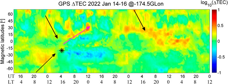
FIGURE 3. UT and MLat variations of GPS-observed residual TEC (ΔTEC). The residual TEC is obtained by a ratio between TEC on January 14–16 and the average TEC on January 9–13. ΔTEC is given in logarithm based on 10. The black and magenta arrows represent the LSTIDs.

Previous studies had disclosed that the variations in TEC were mainly controlled by the changes of electron density at an altitude of the highest density (hmF₂) (Liu et al., 2016). The hmF₂ has an average value of ∼300 km in this work (Figures not shown). Thus, the UT versus magnetic latitudes of ΔNe from TIEGCM at −174.5° GLon and ∼300 km is shown in Figure 4. LSTIDs in ΔNe can be found at 22-02 UT and middle latitudes in both hemispheres, as indicated by two black arrows. Comparing Figures 3, 4, we can find that two LSTIDs in ΔTEC are also reproduced in TIEGCM. The large-scale similarity of the equatorward traveling of LSTIDs between modeled and observed results is achieved, which ensures the reliability of TIEGCM in capturing the LSTIDs. However, the tail-like LSTIDs are not well reproduced in TIEGCM, because TIEGCM does not include the effects of huge geohazard events, i.e., a violent volcano eruption.

FIGURE 4

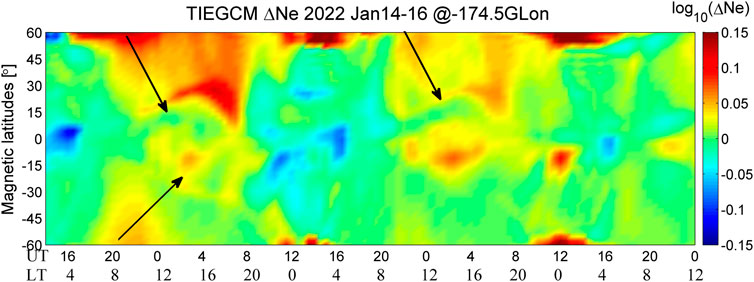
FIGURE 4. Similar to Figure 3, but for the TIEGCM modeled residual Ne (ΔNe) at 300 km.

4 Discussion

Two LSTIDs have been observed in TEC observations from IGS, and confirmed in TEC and Ne simulations from TIEGCM. Previous studies have reported that large-scale ionospheric disturbances might be controlled by several forces, i.e., electric field, auroral heating, and neutral winds (e.g., Shiokawa et al., 2007; Katamzi-Joseph et al., 2019). Which one might be responsible for these two LSTIDs during storm periods? It is still unknown. Using TIEGCM, the potential drivers of two LSTIDs and their interhemispheric asymmetry have been disclosed in this work.

4.1 Term analysis of O⁺ continuity

Similar to the method used in previous studies (Liu et al., 2016; Qian et al., 2016; Zhang et al., 2021), a term analysis of the ionospheric O⁺ continuity equation (see Eq. 1) was performed in this work, to determine the relative contributions from neutral winds, chemical processes (including chemical production and loss rate), plasma drifts, and ambipolar diffusion.

$\raisebox{1ex}{$\partial N$}\!\left/ \!\raisebox{-1ex}{$\partial t$}\right.=q-\beta N-\nabla \bullet \left(NV\right)(1)$

where $\raisebox{1ex}{$\partial N$}\!\left/ \!\raisebox{-1ex}{$\partial t$}\right.$, q, $\beta N$, and $\nabla \bullet \left(NV\right)$ are the change rate of ionospheric main ions of O⁺, chemical production rate, loss rate, and effects from transport processes (including neutral winds, E × B drifts, and ambipolar diffusion), respectively. During the magnetic storm on January 14–16, 2022, the influences from chemical processes (both chemical production and loss rate) and ambipolar diffusion on O⁺ changes in the formation of LSTIDs are much weaker than that from E× B drifts and neutral winds (Figures not shown). Thus, only effects from E × B drifts and neutral winds are investigated in the following.

Figure 5 shows the UT versus magnetic latitudes of total O⁺ changes due to all forcing terms, E × B drifts, and neutral winds at ∼300 km and −174.5° GLon. In Figure 5A, the O⁺ changes due to forcing terms at middle latitudes in both hemispheres also show similar structures with LSTIDs in ΔNe at the end of January 14. The total O⁺ changes in the traveling path of LSTIDs in the northern hemisphere have an average value of ∼5 cm⁻³s⁻¹. In the southern hemisphere, the average value of the total O⁺ changes is weaker (∼2 cm⁻³s⁻¹) than that in the northern hemisphere. At the end of January 15, similar LSTIDs in total O⁺ changes at middle latitudes in the northern hemisphere can be found, ensuring the occurrence of LSTIDs in ΔNe.

FIGURE 5

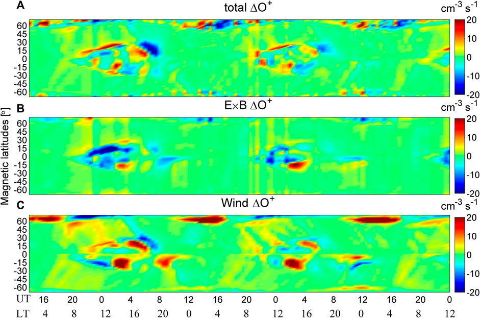
FIGURE 5. The magnetic latitudes and UT variations of total residual O⁺ (ΔO⁺) (A), ΔO⁺ due to E × B (B), and ΔO⁺ due to neutral winds (C) at ∼300 km and −174.5° GLon on January 14–16, 2022. ΔO⁺ is obtained by removing the background quiet-time O⁺. ΔO⁺ is given in cm⁻³s⁻¹.

Previous studies have reported the effects of Lorenz force due to the penetration of electric field on the equatorward LSTIDs (Borries et al., 2016). Figure 5B depicts the effects of E × B drifts on the O⁺ changes. It can be found that the average value of the O⁺ changes is ∼3 and ∼2 cm⁻³s⁻¹ in the LSTIDs in the northern and southern hemispheres, respectively. However, there is not a significant time delay with respect to latitudes. The disturbances of O⁺ due to E × B drifts occur simultaneously at almost all latitudes (Zhang et al., 2019). Thus, we can conclude here that E × B drifts play negligible roles in the equatorward propagation of LSTIDs, but could contribute to the enhancement of ΔNe (Figure 5B). The ΔO⁺ enhancement owing to the plasma transport from E × B drifts supports the occurrence of LSTIDs.

The neutral winds play important roles in the vertical movement of ionospheric plasma (Liu et al., 2016; Zhang et al., 2019). Because thermospheric winds could move the charged ions upward/downward along the geomagnetic field lines, causing the enhancement/depletion of ionospheric plasma due to the chemical recombination (Rishbeth, 1967; Zhang et al., 2012). To disclose the roles of neutral winds, Figure 5C shows the O⁺ changes due to neutral winds at −174.5° GLon and ∼300 km during the disturbed time. In Figures 5A, C corresponding O⁺ enhancement due to neutral winds occurs at the traveling path of LSTIDs in both hemispheres. The mean value of LSTIDs in O⁺ changes is approximately 6 and 3 cm⁻³s⁻¹ in the northern and southern hemispheres, respectively. A comparison between Figures 5A, C indicates that the LSTIDs in ΔNe is dominated by thermospheric winds. Figure 6 illustrates the UT and magnetic latitude variations of meridional wind disturbances at −174.5° GLon and ∼300 km during disturbed periods. As indicated by three black arrows, the LSTADs in the equatorward winds can be found. The average speed of LSTADs at the end of January 14 in the northern and southern hemispheres is ∼30 and ∼25 m/s, respectively. The magnitude of LSTADs at the end of January 15 in the northern hemisphere is smaller (∼20 m/s) than that at the end of January 14.

FIGURE 6

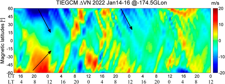
FIGURE 6. UT and MLat variations of TIEGCM-modeled meridional wind disturbances (ΔVN). ΔVN is the difference between VN during the disturbed and quiet time. ΔVN is given in m/s. Positive value stands for northward winds.

The interhemispheric asymmetry of LSTIDs might be attributed to the meridional wind disturbances, which are stronger in the northern hemisphere than that in the southern hemisphere. The vertical plasma drifts due to meridional winds are expressed as follows (Eq. 2; Zhang et al., 2012):

$\text{VV}=v_{n}cosDcos\left|I\right|\sin \left|I\right|(2)$

where $\text{VV}$, $v_n$, $D$ and $I$ are plasma drifts, thermospheric meridional winds, magnetic declination, and inclination, respectively. In general, the stronger meridional wind disturbances might mean the faster vertical plasma drifts. Thus, owing to the faster equatorward winds, more plasma at lower altitudes can be transported to higher altitudes where the chemical recombination could be slower, generating a stronger disturbance in ionospheric plasma density. Thus, the magnitude of LSTIDs at the end of January 14 is stronger in the northern hemisphere than that in the southern hemisphere. Furthermore, the disturbances in meridional winds at the end of January 15 in the southern hemisphere are not strong enough to push enough plasma up to higher altitudes, hence the LSTIDs do not occur.

4.2 Vertical profile

Previous studies have reported the features of LSTIDs observed at different altitudes, e.g., incoherent scatter radar measurements at ∼325 km, Swarm-observed plasma at ∼460 and ∼540 km, CHAMP-observed electron density at ∼400 km, and GPS-observed TEC (Shiokawa et al., 2002; Lei et al., 2008; Borries et al., 2016). As discussed before, the thermospheric meridional winds are responsible for the LSTIDs in both hemispheres via moving plasma upward along the geomagnetic field lines. In Figure 4, LSTIDs in ΔNe at ∼23 UT on January 14 are located at approximately ±40°∼±50° MLat. To investigate the altitudinal variations, Figure 7 gives the vertical mean profile of ΔNe, modeled Ne, ΔO⁺ due to neutral winds, and meridional wind disturbances (ΔVN) at 23 UT within ±40° to ±50° MLat. In Figure 7A, ΔNe is enhanced at altitudes higher than 200 km. The maximum intensity of ΔNe is ∼3.5 × 10¹⁰ m⁻³ and ∼1.4 × 10¹⁰ m⁻³ in the northern and southern hemispheres, respectively. The altitude of maximum ΔNe is at ∼250 (∼270) km in the northern (southern) hemisphere, which might be attributed to the equatorward winds and background plasma (Afraimovich et al., 2008). As shown in Figure 7B, the background plasma density is the strongest at ∼230 and ∼240 km in the northern and southern hemispheres, respectively. A stronger background plasma could generate stronger LSTIDs in ΔNe (Ding et al., 2007), hence the strongest LSTIDs in ΔNe at ∼250 and ∼270 in the northern and southern hemispheres. During the disturbed period, ΔO⁺ due to neutral winds at middle latitudes is negative at low altitudes below 220 km, and positive at high altitudes >220 km (Figure 7C). Owing to the thermospheric equatorward winds (Figure 7D), the ionospheric charged ions are moved upward along the geomagnetic field lines to a higher altitude with slower chemical recombination (Zhang SR et al., 2022), resulting in an enhancement of plasma at a higher altitude above ∼220 km. Furthermore, the altitude differences between the maxima of ΔNe and background plasma is ∼20 and 30 km in the northern and southern hemispheres, respectively. This interesting phenomenon can be attributed to the wind transport effects.

FIGURE 7

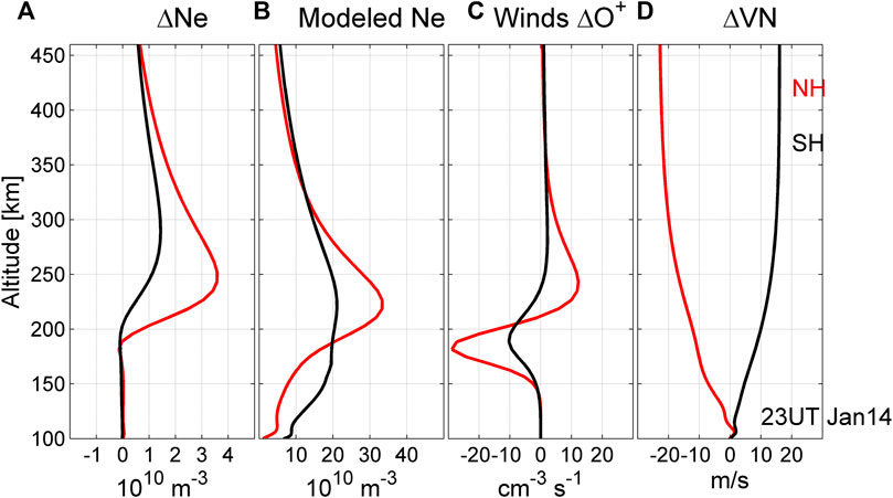
FIGURE 7. The vertical profile of ΔNe (A), modeled Ne (B), ΔO⁺ due to neutral winds (C), and meridional wind disturbances [(D), ΔVN] at −174.5° GLon and 23 UT on 14 January 2022. The red and black lines represent northern and southern hemispheres, respectively.

An interhemispheric asymmetry also occurs in the altitudinal profile of LSTIDs in ΔNe. This might be related to two potential reasons. One is the equatorward wind disturbances, which shows interhemispheric asymmetry (Figure 7D). The other might be the stronger background plasma in the northern hemisphere than that in the southern hemisphere (Figure 7B). Owing to both the stronger ΔVN and background plasma, stronger LSTIDs occur in the northern hemisphere than that in the southern hemisphere (Zhang SR et al., 2012). The altitude differences between the maximum ΔNe and background plasma is smaller in the southern hemisphere than that in the northern hemisphere.

5 Conclusion

Using observations from GPS, and numerical simulations from TIEGCM, the LSTIDs in ΔNe and its interhemispheric asymmetry and altitudinal profile are investigated. Several interesting results are found.

1. The TIEGCM simulations show that the thermospheric equatorward winds are responsible for the LSTIDs. The interhemispheric asymmetry in plasma disturbances is related to the corresponding asymmetry in the meridional wind disturbances.

2. The vertical profile of ΔNe is also shown in this work, which is attributed to both the background plasma and transport effects from equatorward winds. The interhemispheric asymmetry also occurs in the altitudinal profile and is attributed to two factors: the background electron density and equatorward winds.

3. A tail-like LSTIDs is shown in the GPS-observed TEC after the eruption of the Tonga volcano, however, it is not reproduced by TIEGCM. The potential reason might be the huge geohazard event that is not included in the numerical physical model, and deserve further exploration in the future.

Data availability statement

The original contributions presented in the study are included in the article/Supplementary material, further inquiries can be directed to the corresponding author.

Author contributions

KZ: Data curation, Writing–original draft. HW: Writing–review and editing.

Funding

The author(s) declare financial support was received for the research, authorship, and/or publication of this article. We are grateful for the sponsor from the National Natural Science Foundation of China Basic Science Center (42188101), the Fundamental Research Funds for the Central Universities (2042023kf0099), the National Nature Science Foundation of China (No. 41974182 and 42122031). This work is supported by Hubei Provincial Natural Science Foundation of China (2023AFB616). This work is also supported by the Project Supported by the Specialized Research Fund for State Key Laboratories.

Conflict of interest

The authors declare that the research was conducted in the absence of any commercial or financial relationships that could be construed as a potential conflict of interest.

Publisher’s note

All claims expressed in this article are solely those of the authors and do not necessarily represent those of their affiliated organizations, or those of the publisher, the editors and the reviewers. Any product that may be evaluated in this article, or claim that may be made by its manufacturer, is not guaranteed or endorsed by the publisher.

References

Afraimovich, E. L., Kosogorov, E. A., Leonovich, L. A., Palamartchouk, K. S., Perevalova, N. P., and Pirog, O. M. (2000). Determining parameters of large-scale traveling ionospheric disturbances of auroral origin using GPS-arrays. J. Atmos. Solar-Terrestrial Phys. 62 (7), 553–565. doi:10.1016/s1364-6826(00)00011-0

CrossRef Full Text | Google Scholar

Afraimovich, E. L., Voeykov, S. V., Perevalova, N. P., and Ratovsky, K. G. (2008). Large-scale traveling ionospheric disturbances of auroral origin according to the data of the GPS network and ionosondes. Adv. Space Res. 42 (7), 1213–1217. doi:10.1016/j.asr.2007.11.023

CrossRef Full Text | Google Scholar

Balthazor, R. L., and Moffett, R. J. (1997). A study of atmospheric gravity waves and travelling ionospheric disturbances at equatorial latitudes. Ann. Geophys. 15 (8), 1048–1056. doi:10.1007/s00585-997-1048-4

CrossRef Full Text | Google Scholar

Borries, C., Mahrous, A. M., Ellahouny, N. M., and Badeke, R. (2016). Multiple ionospheric perturbations during the Saint Patrick's Day storm 2015 in the European-African sector. J. Geophys. Res. Space Phys. 121 (11), 11–333. doi:10.1002/2016ja023178

CrossRef Full Text | Google Scholar

Bruinsma, S. L., and Forbes, J. M. (2009). Properties of traveling atmospheric disturbances (TADs) inferred from CHAMP accelerometer observations. Adv. Space Res. 43 (3), 369–376. doi:10.1016/j.asr.2008.10.031

CrossRef Full Text | Google Scholar

Cherniak, I., and Zakharenkova, I. (2018). Large-scale traveling ionospheric disturbances origin and propagation: case study of the December 2015 geomagnetic storm. Space weather 16 (9), 1377–1395. doi:10.1029/2018sw001869

CrossRef Full Text | Google Scholar

Ding, F., Wan, W., Ning, B., and Wang, M. (2007). Large-scale traveling ionospheric disturbances observed by GPS total electron content during the magnetic storm of 29–30 October 2003. J. Geophys. Res. Space Phys. 112 (6), 309. doi:10.1029/2006ja012013

CrossRef Full Text | Google Scholar

Dungey, J. W. (1961). Interplanetary magnetic field and the auroral zones. Phys. Rev. Lett. 6 (2), 47–48. doi:10.1103/physrevlett.6.47

CrossRef Full Text | Google Scholar

Hagan, M. E., and Forbes, J. M. (2002). Migrating and nonmigrating diurnal tides in the middle and upper atmosphere excited by tropospheric latent heat release. J. Geophys. Res. Atmos. 107 (24), 4754. doi:10.1029/2001jd001236

CrossRef Full Text | Google Scholar

Hagan, M. E., and Forbes, J. M. (2003). Migrating and nonmigrating semidiurnal tides in the upper atmosphere excited by tropospheric latent heat release. J. Geophys. Res. Space Phys. 108 (2), 1062. doi:10.1029/2002ja009466

CrossRef Full Text | Google Scholar

Heelis, R. A., Lowell, J. K., and Spiro, R. W. (1982). A model of the high-latitude ionospheric convection pattern. J. Geophys. Res. Space Phys. 87 (8), 6339–6345. doi:10.1029/ja087ia08p06339

CrossRef Full Text | Google Scholar

Hernández-Pajares, M., Juan, J. M., Sanz, J., Orus, R., Garcia-Rigo, A., Feltens, J., et al. (2009). The IGS VTEC maps: a reliable source of ionospheric information since 1998. J. Geodesy 83, 263–275. doi:10.1007/s00190-008-0266-1

CrossRef Full Text | Google Scholar

Hocke, K., and Schlegel, K. (1996). A review of atmospheric gravity waves and travelling ionospheric disturbances: 1982–1995. Ann. Geophys. 14 (9), 917. doi:10.1007/s005850050357

CrossRef Full Text | Google Scholar

Jonah, O. F., Zhang, S., Coster, A. J., Goncharenko, L. P., Erickson, P. J., and Rideout, W., (2020). Understanding inter-hemispheric traveling ionospheric disturbances and their mechanisms. Remote Sens. 12 (2), 228. doi:10.3390/rs12020228

CrossRef Full Text | Google Scholar

Katamzi-Joseph, Z. T., Aruliah, A. L., Oksavik, K., Habarulema, J. B., Kauristie, K., and Kosch, M. J. (2019). Multi-instrument observations of large-scale atmospheric gravity waves/traveling ionospheric disturbances associated with enhanced auroral activity over Svalbard. Adv. Space Res. 63 (1), 270–281. doi:10.1016/j.asr.2018.08.042

CrossRef Full Text | Google Scholar

Lei, J., Burns, A. G., Tsugawa, T., Wang, W., Solomon, S. C., and Wiltberger, M. (2008). Observations and simulations of quasiperiodic ionospheric oscillations and large-scale traveling ionospheric disturbances during the December 2006 geomagnetic storm. J. Geophys. Res. Space Phys. 113 (6), 310. doi:10.1029/2008ja013090

CrossRef Full Text | Google Scholar

Lin, C. H., Richmond, A. D., Heelis, R. A., Bailey, G. J., Lu, G., Liu, J. Y., et al. (2005). Theoretical study of the low-and midlatitude ionospheric electron density enhancement during the October 2003 superstorm: relative importance of the neutral wind and the electric field. J. Geophys. Res. Space Phys. 110 (A12), 312. doi:10.1029/2005ja011304

CrossRef Full Text | Google Scholar

Liu, J., Liu, L., Nakamura, T., Zhao, B., Ning, B., and Yoshikawa, A. (2014). A case study of ionospheric storm effects during long-lasting southward IMF Bz-driven geomagnetic storm. J. Geophys. Res. Space Phys. 119 (9), 7716–7731. doi:10.1002/2014ja020273

CrossRef Full Text | Google Scholar

Liu, J., Wang, W., Burns, A., Yue, X., Zhang, S., Zhang, Y., et al. (2016). Profiles of ionospheric storm-enhanced density during the 17 March 2015 great storm. J. Geophys. Res. Space Phys. 121 (1), 727–744. doi:10.1002/2015ja021832

CrossRef Full Text | Google Scholar

MacDougall, J. W., and Jayachandran, P. T. (2011). Solar terminator and auroral sources for traveling ionospheric disturbances in the midlatitude F region. J. Atmos. solar-terrestrial Phys. 73 (17-18), 2437–2443. doi:10.1016/j.jastp.2011.10.009

CrossRef Full Text | Google Scholar

Munro, G. H. (1958). Travelling ionospheric disturbances in the F region. Aust. J. Phys. 11 (1), 91–112. doi:10.1071/ph580091

CrossRef Full Text | Google Scholar

Nicolls, M. J., Vadas, S. L., Meriwether, J. W., Conde, M. G., and Hampton, D. (2012). The phases and amplitudes of gravity waves propagating and dissipating in the thermosphere: application to measurements over Alaska. J. Geophys. Res. Space Phys. 117 (5), 323. doi:10.1029/2012ja017542

CrossRef Full Text | Google Scholar

Nishimura, Y., Zhang, S. R., Lyons, L. R., Deng, Y., Coster, A. J., Moen, J. I., et al. (2020). Source region and propagation of dayside large-scale traveling ionospheric disturbances. Geophys. Res. Lett. 47 (19), 619. doi:10.1029/2020gl089451

CrossRef Full Text | Google Scholar

Ogwala, A., Oyedokun, O. J., Ogunmodimu, O., Akala, A. O., Ali, M. A., Jamjareegulgarn, P., et al. (2022). Longitudinal variations in equatorial ionospheric TEC from GPS, global ionosphere map and international reference ionosphere-2016 during the descending and minimum phases of solar cycle 24. Universe 8 (11), 575. doi:10.3390/universe8110575

CrossRef Full Text | Google Scholar

Panda, S. K., Haralambous, H., and Kavutarapu, V. (2018). Global longitudinal behavior of IRI bottomside profile parameters from FORMOSAT-3/COSMIC ionospheric occultations. J. Geophys. Res. Space Phys. 123 (8), 7011–7028. doi:10.1029/2018ja025246

CrossRef Full Text | Google Scholar

Panda, S. K., Harikaa, B., Vineetha, P., Kumar Dabbakutib, J. R. K., Akhila, S., and Srujanaa, G. Validity of different global ionospheric TEC maps over Indian region. 2021 3rd International Conference on Advances in Computing, Communication Control and Networking (ICAC3N), Greater Noida, India, 2021, 1749–1755.

Google Scholar

Perlongo, N. J., Ridley, A. J., Cnossen, I., and Wu, C. (2018). A year-long comparison of GPS TEC and global ionosphere-thermosphere models. J. Geophys. Res. Space Phys. 123 (2), 1410–1428. doi:10.1002/2017ja024411

CrossRef Full Text | Google Scholar

Pi, X., Mendillo, M., Hughes, W. J., Buonsanto, M. J., Sipler, D. P., Kelly, J., et al. (2000). Dynamical effects of geomagnetic storms and substorms in the middle-latitude ionosphere: an observational campaign. J. Geophys. Res. Space Phys. 105 (4), 7403–7417.

Google Scholar

Qian, L., Burns, A. G., Wang, W., Solomon, S. C., Zhang, Y., and Hsu, V. (2016). Effects of the equatorial ionosphere anomaly on the interhemispheric circulation in the thermosphere. J. Geophys. Res. Space Phys. 121 (3), 2522–2530. doi:10.1002/2015ja022169

CrossRef Full Text | Google Scholar

Rajesh, P. K., Lin, C. H., Lin, C. Y., Chen, C. H., Liu, J. Y., and Matsuo, T., (2021). Extreme positive ionosphere storm triggered by a minor magnetic storm in deep solar minimum revealed by FORMOSAT-7/COSMIC-2 and GNSS observations. J. Geophys. Res. Space Phys. 126 (2), 2020JA028261. doi:10.1029/2020ja028261

CrossRef Full Text | Google Scholar

Richards, P. G., Fennelly, J. A., and Torr, D. G. (1994). EUVAC: a solar EUV flux model for aeronomic calculations. J. Geophys. Res. Space Phys. 99 (5), 8981–8992. doi:10.1029/94ja00518

CrossRef Full Text | Google Scholar

Rishbeth, H. (1967). The effect of winds on the ionospheric F2-peak. J. Atmos. Terr. Phys. 29 (3), 225–238. doi:10.1016/0021-9169(67)90192-4

CrossRef Full Text | Google Scholar

Shiokawa, K., Lu, G., Otsuka, Y., Ogawa, T., Yamamoto, M., Nishitani, N., et al. (2007). Ground observation and AMIE-TIEGCM modeling of a storm-time traveling ionospheric disturbance. J. Geophys. Res. Space Phys. 112 (5), 308. doi:10.1029/2006ja011772

CrossRef Full Text | Google Scholar

Shiokawa, K., Mori, M., Otsuka, Y., Oyama, S., Nozawa, S., Suzuki, S., et al. (2013). Observation of nighttime medium-scale travelling ionospheric disturbances by two 630-nm airglow imagers near the auroral zone. J. Atmos. Solar-Terrestrial Phys. 103, 184–194. doi:10.1016/j.jastp.2013.03.024

CrossRef Full Text | Google Scholar

Shiokawa, K., Otsuka, Y., Ogawa, T., Balan, N., Igarashi, K., Ridley, A. J., et al. (2002). A large-scale traveling ionospheric disturbance during the magnetic storm of 15 September 1999. J. Geophys. Res. Space Phys. 107 (6), 1088. doi:10.1029/2001ja000245

CrossRef Full Text | Google Scholar

Shiokawa, K., Otsuka, Y., Ogawa, T., Kawamura, S., Yamamoto, M., Fukao, S., et al. (2003). Thermospheric wind during a storm-time large-scale traveling ionospheric disturbance. J. Geophys. Res. Space Phys. 108 (12), 1052. doi:10.1029/2003ja010001

CrossRef Full Text | Google Scholar

Wang, W., Talaat, E. R., Burns, A. G., Emery, B., Hsieh, S. Y., Lei, J., et al. (2012). Thermosphere and ionosphere response to subauroral polarization streams (SAPS): model simulations. J. Geophys. Res. Space Phys. 117 (7), 301. doi:10.1029/2012ja017656

CrossRef Full Text | Google Scholar

Weimer, D. R. (2005). Improved ionospheric electrodynamic models and application to calculating Joule heating rates. J. Geophys. Res. Space Phys. 110 (5), 306. doi:10.1029/2004ja010884

CrossRef Full Text | Google Scholar

Wu, Q., Sheng, C., Wang, W., Noto, J., Kerr, R., McCarthy, M., et al. (2019). The midlatitude thermospheric dynamics from an interhemispheric perspective. J. Geophys. Res. Space Phys. 124 (10), 7971–7983. doi:10.1029/2019ja026967

CrossRef Full Text | Google Scholar

Yin, F., Lühr, H., Park, J., and Wang, L. (2019). Comprehensive analysis of the magnetic signatures of small-scale traveling ionospheric disturbances, as observed by Swarm. J. Geophys. Res. Space Phys. 124 (12), 10794–10815. doi:10.1029/2019ja027523

CrossRef Full Text | Google Scholar

Zhang, K., Liu, J., Wang, W., and Wang, H. (2019c). The effects of IMF B periodic oscillations on thermospheric meridional winds. J. Geophys. Res. Space Phys. 124 (7), 5800–5815. doi:10.1029/2019ja026527

CrossRef Full Text | Google Scholar

Zhang, K., Wang, H., Liu, J., Zheng, Z., He, Y., Gao, J., et al. (2021b). Dynamics of the tongue of ionizations during the geomagnetic storm on September 7, 2015. J. Geophys. Res. Space Phys. 126 (6), 2020JA029038. doi:10.1029/2020ja029038

CrossRef Full Text | Google Scholar

Zhang, K., Wang, H., Yamazaki, Y., and Xiong, C. (2021a). Effects of subauroral polarization streams on the equatorial electrojet during the geomagnetic storm on June 1, 2013. J. Geophys. Res. Space Phys. 126 (10), 2021JA029681. doi:10.1029/2021ja029681

CrossRef Full Text | Google Scholar

Zhang, K., Wang, W., Wang, H., Dang, T., Liu, J., and Wu, Q. (2018). The longitudinal variations of upper thermospheric zonal winds observed by the CHAMP satellite at low and midlatitudes. J. Geophys. Res. Space Phys. 123 (11), 9652–9668. doi:10.1029/2018ja025463

CrossRef Full Text | Google Scholar

Zhang, S. R., Coster, A. J., Erickson, P. J., Goncharenko, L. P., Rideout, W., and Vierinen, J. (2019a). Traveling ionospheric disturbances and ionospheric perturbations associated with solar flares in September 2017. J. Geophys. Res. Space Phys. 124 (7), 5894–5917. doi:10.1029/2019ja026585

CrossRef Full Text | Google Scholar

Zhang, S. R., Erickson, P. J., Coster, A. J., Rideout, W., Vierinen, J., Jonah, O., et al. (2019b). Subauroral and polar traveling ionospheric disturbances during the 7–9 September 2017 storms. Space weather 17 (12), 1748–1764. doi:10.1029/2019sw002325

CrossRef Full Text | Google Scholar

Zhang, S. R., Foster, J. C., Holt, J. M., Erickson, P. J., and Coster, A. J. (2012). Magnetic declination and zonal wind effects on longitudinal differences of ionospheric electron density at midlatitudes. J. Geophys. Res. Space Phys. 117 (8), 329. doi:10.1029/2012ja017954

CrossRef Full Text | Google Scholar

Zhang, S. R., Vierinen, J., Aa, E., Goncharenko, L. P., Erickson, P. J., Rideout, W., et al. (2022). 2022 Tonga volcanic eruption induced global propagation of ionospheric disturbances via Lamb waves. Front. Astronomy Space Sci. 9, 871275. doi:10.3389/fspas.2022.871275

CrossRef Full Text | Google Scholar