Testing adiabatic models of energetic electron acceleration at dipolarization fronts

Betatron acceleration is commonly cited as a primary accelerator of energetic electrons at dipolarization fronts, and many case studies compare observed energetic electrons measurements to a betatron model. In this work, we extend this to a statistical study. We identified 168 dipolarizations with an enhanced flux of energetic electrons at Magnetospheric Multiscale (MMS). We compared the observed flux of energetic electrons above 1 keV to a betatron acceleration model assuming a source population similar to the population in the quiet plasma sheet and found that, on average, the model slightly overestimated the observation, but there was a wide spread of errors. We then tested characteristics such as position, change in and strength of magnetic field, and wave power to determine if any of these characteristics affected the accuracy of the model; the only clear correlations were that the model was less accurate when the initial total magnetic field was smaller and when there was a higher E_y during the dipolarization. Since the betatron model did not explain our observations very well, we repeated with a full adiabatic model that included a Fermi acceleration component as well. We found that the adiabatic model slightly underestimated the observations, but with a smaller error than the betatron model under the same assumptions. Testing the same parameters, we found that the adiabatic model also did not strongly rely on any of the parameters except the initial magnetic field, and the anti-correlation with E_y was no longer present. The fact that neither model was generally applicable means that either adiabatic processes alone are not enough to explain electron acceleration at dipolarization fronts in general, or the common assumption we used, that the source population has the same phase space density as the cold pre-existing population, is not valid.

1 Introduction

Dipolarization fronts (DFs) are characterized by rapid increases in the z-component of the magnetic field in the magnetotail (e.g., Russell and McPherron, 1973; Angelopoulos et al., 1992; Nakamura et al., 2002). As the name suggests, these fronts carry a more dipolar field than the surrounding stretched tail field. The dipolarization of the tail is associated with substorms (e.g., Baumjohann et al., 1999; Fu et al., 2020, and references therein). When reconnection occurs in the tail, it is often accompanied by high-speed earthward flows such as bursty bulk flows (BBFs) (e.g., Angelopoulos et al., 1992). Embedded in BBFs are dipolarizing flux bundles (DFBs), which are smaller flux tubes that carry a more dipolar field than the surrounding plasma (e.g., Liu et al., 2014). The kinetic-scale boundaries between DFBs and the ambient plasma are known as dipolarization fronts (DFs), They are often considered as a tangential discontinuity at the boundary between the dipolar field and stretched field (e.g., Sergeev et al., 2009; Fu H. S. et al., 2012). The high B_z region behind the DF is called the flux pileup region. As DFs travel earthward, they deflect the plasma into which they are traveling and evolve in a way that is coupled with the flow (e.g., Nakamura et al., 2002).

Dipolarization fronts are fairly common, with about five events per day observed at the most active region of the magnetotail, X ∼-15 R_E (Liu et al., 2013; Xiao et al., 2017), which is comparable to the occurrence rate of substorms, furthering the link between substorms and DFs (Fu et al., 2012a). DFs are more common on the dusk side and at times of high geomagnetic activity. It is also common for multiple DFs to occur at a time, with about a third of DFs occurring within 15 min of another one (Xiao et al., 2017). The average thickness of a DF is a few hundred km, or ∼1.5-2 ion inertial lengths (Runov et al., 2009; Hwang et al., 2011; Runov et al., 2011; Schmid et al., 2011; Fu et al., 2012a), although DFs that propagate faster tend to be thicker (Schmid et al., 2016). They are also generally localized in the tail, with a width of around 1–3 R_E (e.g., Sergeev et al., 1996; Nakamura et al., 2004). With increased propagation speed, DFs tend to have a higher B_z and E_y, so there is a higher flux transport rate (Schmid et al., 2016). Schmid et al. (2016) found DFs were more likely to be faster near Earth than in the midtail, contrary to assumptions about fronts slowing as they approach Earth. This could be a data artifact from different conditions for the two samples or a result of only DFBs with extremely low entropy being able to penetrate that deeply. There is often a characteristic dip in B_z before it increases in the dipolarization, likely as a result of diamagnetic or field-aligned currents; however, it is possible for events with negative dips to evolve into events with positive dips since the dips below 0 occur farther from Earth (Schmid et al., 2019).

Energetic electron flux increases at dipolarizations has been reported and can range from a 2–3 times increase (Runov et al., 2011) to a 5 times increase (Gabrielse et al., 2014) to 2–4 orders of magnitude increase (Wu et al., 2013) while fluxes of electrons at lower energies (∼a few keV) decrease (Hwang et al., 2011; Turner et al., 2016). The mechanism that accelerates these electrons is a topic of much study, with betatron and Fermi acceleration often viewed as the primary mechanisms (e.g., Williams et al., 1990; Liu et al., 2017a). Both mechanisms are adiabatic acceleration processes. Betatron acceleration is a result of the conservation of the first adiabatic invariant and accelerates particles as the magnetic field strength increases. Fermi acceleration is a result of the conservation of the second adiabatic invariant and accelerates particles as the length of flux tubes decrease. Another form of Fermi acceleration seen in the tail comes in “reflections”, which is analogous to the classical system of a ball gaining energy as it bounces off two walls moving towards each other (Drake et al., 2006; Arnold et al., 2021; Turner et al., 2021). Pitch angle distributions (PADs) are an important tool to distinguish between these two types of acceleration. Since betatron acceleration acts on perpendicular particles, it produces PADs peaked around 90°, sometimes called a “pancake distribution” (e.g., Wu et al., 2006; Khotyaintsev et al., 2011). On the other hand, Fermi acceleration acts on parallel particles, so it produces a field-aligned and anti-field-aligned distribution, known as a “cigar distribution” (e.g., Williams et al., 1990; Wu et al., 2006). A combination of Fermi and betatron acceleration can produce a “rolling pin distribution” that has peaks around 0°, 90°, and 180° (Liu et al., 2017a). An alternate interpretation of adiabatic acceleration is that the particles are being accelerated directly by the electric field of the DF (Fu et al., 2012b). In addition to these adiabatic methods, particles could be accelerated by interactions with turbulent reconnection exhaust (Ergun et al., 2020a; Ergun et al., 2020b) or wave-particle interactions. Various types of waves have been observed at DFs, including lower hybrid drift (LHD) waves, whistler-mode waves, and electron cyclotron harmonic (ECH) waves. LHD waves are typically observed at the front boundary itself (e.g., Zhou et al., 2009; Khotyaintsev et al., 2011; Chen et al., 2021). ECH waves have generally been observed following the front (e.g., Zhou et al., 2009) but are highly correlated with DFs, as in one study $>$50% of ECH waves observed were correlated with DFs (Zhang and Angelopoulos, 2014). Whistler waves are also commonly found with DFs, most often after the front in the flux pileup region (e.g., Khotyaintsev et al., 2011; Viberg et al., 2014; Chen et al., 2021), although there have been cases where they have been observed at the front itself and in regions throughout the dipolarization (Huang et al., 2012; Chen et al., 2021). Whistler waves are found in up to 60% of all DFs, though more often when B_x is close to 0 (Viberg et al., 2014), and can be driven by a temperature anisotropy with T_⊥/T_‖ > 1, which is evidence for betatron acceleration increasing T_⊥ (Khotyaintsev et al., 2011).

Different studies do not always agree on the relative importance of betatron and Fermi acceleration at DFs. Using simple magnetic field measurements, multiples studies have found that betatron acceleration sufficiently described the energetic electron flux (Asano et al., 2010; Turner et al., 2016; Malykhin et al., 2018). Turner et al. (2016) found this held within the range of ∼10–100 keV, while Malykhin et al. (2018) found it held up to 90 keV. Alternatively, Smets et al. (1999) found that Fermi acceleration was the leading process by analyzing PADs and Fu et al. (2022) found that Fermi acceleration alone was responsible for electron acceleration, by analyzing the PADs and magnetic field geometry. However, many studies found that both betatron and Fermi acceleration were required to describe electron acceleration. Many studies simply use a combination of betatron and Fermi acceleration, like Pan et al. (2012) comparing observations to a simple models for change in particle energy, Birn et al. (2013) using simulations, or Tang et al. (2020) describing PADs with a combination of betatron, Fermi, and a loss cone from the magnetic mirror configuration. Other studies investigate where different mechanisms are dominant in more detail. From observations and simple models, Fu et al. (2011) found betatron acceleration in the decaying flux pileup region and Fermi acceleration in the growing flux pileup region, although adiabatic acceleration did not explain acceleration at $<$20 keV. Vaivads et al. (2021) found betatron acceleration in the magnetic flux pileup region and Fermi acceleration, wave-particle interactions, and direct acceleration from the electric field in the flux rope ahead of the pileup region. Ma et al. (2020) calculated the acceleration rates directly and found that betatron acceleration was dominant but localized, while Fermi acceleration was less effective but present over a wider area. Wu et al. (2013) analyzed PADs to find that betatron acceleration was dominant in the midtail, but the near-Earth region was balanced between betatron and Fermi acceleration. Liu et al. (2017a) analyzed PADs as well and explained them with local betatron acceleration and global-scale Fermi acceleration. There are also studies that claim adiabatic mechanisms alone are not fully capable of describing electron acceleration. Whistler waves near DFs can effectively interact with and accelerate electrons, so using a purely adiabatic model without waves may be inadequate (Zhang et al., 2018). Waves can also affect PADs, especially by isotropizing them (Khotyaintsev et al., 2011), which can harm the reliability of using PADs to determine the adiabatic acceleration mechanism. Energy exchange can also be a non-adiabatic method that produces particle populations similar to betatron acceleration. Moderated by whistler waves, lower-energy electrons can transfer energy to a higher-energy population and can create an enhancement of perpendicular electrons in our energy range of interest (Shklyar, 2017), which is a process that has been observed at DFs (Grigorenko et al., 2020; Grigorenko et al., 2023). Finally, waves scattering electrons into the loss cone can cause an overestimate of the observed flux if we do not take this process into account.

Many different analysis methods are used to determine the dominant acceleration mechanisms, and these methods do not always agree, but one common method to test betatron acceleration is to use a simple model to determine the change in energy based on the change in magnetic field, then apply this change in energy to the energy spectrum before the dipolarization and compare it to the observed energy spectrum at the peak of the dipolarization. This method relies on the assumption of a flat phase-space density gradient across the tail, so that the particles measured before the DF have the same PSD as the particles that were accelerated. It also assumes the initial magnetic field is the same at the observation site and the source location so the increase in B in the particles experienced is the same as measured by the satellite. For case studies, evolving the initial energy spectrum with a simple betatron model can match the observed spectrum well (e.g., Asano et al., 2010; Turner et al., 2016), and even a small-scale statistical study found some correlation with this type of model (Malykhin et al., 2018). However, all of these studies are either case studies, or studies of only a few events. In this work, we want to study the viability of using simple models to evolve the spectrum in a systematic way. The aforementioned assumptions, especially about the source population, can have a large influence considering the localized nature of the structures, so this will quantitatively test how well the assumptions hold on a large scale. We survey dipolarization fronts with energetic electron acceleration to create a large-scale statistical study to quantifiably test how well models for both purely betatron and for adiabatic acceleration describe the evolution of the electron energy spectrum.

2 Instruments

The Magnetospheric Multiscale (MMS) mission was launched in 2015 and includes four spacecraft in tight formation (Burch et al., 2016). Starting in 2017, the orbit had an apogee of $\sim 25R_E$ (Fuselier et al., 2016). The MMS tail season (the time of year when apogee is on the nightside) is generally in the Northern hemisphere summer, meaning we can roughly constrain the time range used for our survey.

The primary instrument used to measure energetic electrons for this study was the Fly’s Eye Energetic Particle Spectrometer (FEEPS) (Blake et al., 2016), which is part of the Energetic Particle Detector (EPD) investigation (Mauk et al., 2016). FEEPS measures electrons in the energy range of 25–650 keV. Each spacecraft has two FEEPS units, each of which has 12 eyes, nine for electrons, and each eye has 16 energy channels. The FEEPS instrument observes a nearly complete full sky in about 2.5 s in survey mode. In addition to FEEPS data, we also used the Fast Plasma Investigation (FPI) to cover lower energies up to 30 keV for electrons (Pollock et al., 2016). Each spacecraft has four dual 180-degree tophat spectrometers for electrons, which allow for a 4π-sr field of view. We also required data from the FIELDS instrument suite (Torbert et al., 2016), especially the fluxgate magnetometer (FGM) (Russell et al., 2016a) to measure the magnetic field. To study waves, we also used the search coil magnetometer (Le Contel et al., 2016) and the electric field double probes (Ergun et al., 2016; Lindqvist et al., 2016).

3 Methodology

3.1 Event selection

To compile a list of dipolarization events, we used a method based on Schmid et al. (2011) and Wu et al. (2013) with an additional requirement for energetic electron flux enhancement observed by MMS. We surveyed all MMS data during the tail season from May 1-October 31 of the years 2017–2022¹. We limited our search to times when the spacecraft is at a distance of $>10R_E$ away from Earth and an MLT between 19 and 5; we then used a 3-min sliding window shifted by 90 s so every time in our region of interest is double-counted and there are no two adjacent times that are not studied in the same window. The criteria we used to identify a dipolarization front were:

- ΔB_z > 4 nT

- Maximum elevation angle, θ > 45°, where $\theta ={\tan }^{-1}\left(\frac{B_z}{B_{xy}}\right)$

- Increase in elevation angle, Δθ > 10°

- Maximum earthward flow v_x > 150 km/s

- Maximum plasma β > 0.5 to ensure the spacecraft is in the plasma sheet

- Maximum B_z occurs after the minimum B_z so the dipolarization is propagating towards the spacecraft

We specifically wanted to find electron acceleration at DFs, so we added another condition for the identification of our events. This required the flux of energetic electrons in the FEEPS instrument at the maximum B_z to be at least 5 times greater than the electron flux at the minimum B_z in either the 70-keV energy channel or the 88-keV channel, and for the maximum flux of the 70-keV channel to be $>10$ (cm s sr keV)⁻¹ to ensure the increase is not small-number statistical noise. These energies were chosen because we expect to see energization up to about 100 keV, so these are near the top of that range. Using this method, we found 168 dipolarization events with energetic electron acceleration. The full list of events is given in Supplementary Table S1.

3.2 Models used

The first model we tested was a simple betatron acceleration model. We start with the equation for how a particle is accelerated by a slowly changing magnetic field during betatron acceleration:

$\frac{\mathrm{d}{W}_{\perp }}{\mathrm{d}t}=\mu \frac{\mathrm{d}{B}_z}{\mathrm{d}t},(1)$

where $\mu =\frac{W_{\perp }}{B}$ (Russell et al., 2016b). Since we did not limit our search to regions with low B_x and B_y (it will be shown in Section 5 that this would not have meaningfully changed our conclusions), we cannot approximate $\mu =\frac{W_{\perp }}{B_z}$ like many other studies do. We can directly measure the time derivatives as $\frac{\mathrm{d}B}{\mathrm{d}t}=\frac{\mathrm{\Delta }B}{\mathrm{\Delta }t}=\frac{B_2-B_1}{t_2-t_1}$, so

$\frac{\mathrm{d}{W}_{\perp }}{\mathrm{d}t}=\frac{W_{\perp 1}}{B_{t1}}\frac{B_{z2}-B_{z1}}{\mathrm{\Delta }t}.(2)$

This produces our final equation for energy change as

$W_{\perp 2}=\frac{W_{\perp 1}}{B_{t1}}\left(B_{z2}-B_{z1}\right)+W_{\perp 1},(3)$

where B_z2 is the maximum B_z and W_⊥2 is the perpendicular energy at that time, and B_z1 is the minimum B_z and W_⊥1 is the corresponding perpendicular energy. Essentially, this is removing the assumption that there are no B_x and B_y components of the field, but keeping the assumption that the change in B_z is the only relevant change for accelerating particles. This describes a change in the energy of the particles, but for the purposes of our analysis, it is more useful to compare the change in flux at single energies. To do this, we model the energy spectrum as a piecewise power law, using the power law index between one energy channel and the channel above it for each data point:

$n=\frac{\mathit{log}\left(j_E/j_{E_{\mathit{high}}}\right)}{\mathit{log}\left(E_{\mathit{high}}/E\right)},(4)$

where n is the power law index for the target channel, E is the energy of that channel, j_E1 is the observed electron flux, and E_high and $j_{E_{\mathit{high}}}$ are the energy and flux, respectively, of the energy channel above it. Therefore, we can use Eq. 3 to say $\frac{E_2}{E_1}=\frac{W_{\perp 2}}{W_{\perp 1}}=\frac{B_{z2}-B_{z1}}{B_{t1}}+1$ and find the change in flux at energy E from

$j_2\left(E\right)=j_1\left(E\right){\left(\frac{B_{z2}-B_{z1}}{B_{t1}}+1\right)}^n,(5)$

where j₁, B_z1, and B_t1 are the initial flux, B_z, and B_t at the minimum B_z; j₂ and B_z2 are the final flux and B_z at the maximum B_z; and n is the power law index from Eq. (4).

One potential problem with this initial simplistic model is that betatron acceleration applies to perpendicular electrons, and the flux change in Eq. (5) applies that same acceleration to all electrons. To address this issue, our second model is an adiabatic model that includes a Fermi acceleration component in addition to the betatron acceleration. Fermi acceleration applies to parallel electrons, so a full adiabatic model combining betatron and Fermi acceleration should describe both perpendicular and parallel pitch angles. The model for Fermi acceleration we use is:

$\frac{\mathrm{d}{v}_{\Vert }}{\mathrm{d}t}=-\frac{\mu }{m_e}\frac{\partial B}{\partial s}+\left({\mathbf{v}}_E+{\mathbf{v}}_{\nabla B}\right)\cdot \frac{\mathrm{d}\mathbf{b}}{\mathrm{d}t},(6)$

where $\frac{\partial }{\partial s}=\mathbf{b}\cdot \nabla$, $\mathbf{b}=\frac{\mathbf{B}}{B}$, ${\mathbf{v}}_E=\frac{\mathbf{E}\times \mathbf{B}}{B^2}$, and ${\mathbf{v}}_{\nabla B}=-\frac{\mu }{e}\frac{\mathbf{B}\times \nabla B}{B^2}$ (Northrop, 1963; Birn et al., 2013). This can be converted from a change in parallel velocity to a change in parallel energy:

$\frac{\mathrm{d}{W}_{\Vert }}{\mathrm{d}t}=v_{\Vert }\left[-\mu \frac{\mathbf{B}}{B}\cdot \nabla B+m_e\left(\frac{\mathbf{E}\times \mathbf{B}}{B^2}-\frac{\mu }{e}\frac{\mathbf{B}\times \nabla B}{B^2}\right)\cdot \frac{\mathrm{d}}{\mathrm{d}t}\left(\frac{\mathbf{B}}{B}\right)\right].(7)$

We can then use this to find the change in energy from Fermi acceleration with $W_2=W_1+\frac{\mathrm{d}{W}_{\Vert }}{\mathrm{d}t}\mathrm{\Delta }t$, or the change in flux from Fermi acceleration with

$j_2=j_1{\left(1+\frac{\mathrm{d}{W}_{\Vert }}{\mathrm{d}t}\frac{\mathrm{\Delta }t}{W_1}\right)}^n(8)$

For the purposes of this study, we used the values from before the dipolarization for all the parameters except ∇B. For ∇B, we calculated it using the four MMS spacecraft, and we used the average between the time before the dipolarization and the peak of the dipolarization.

To get a full adiabatic model, we need to take both betatron and Fermi acceleration into account. In general, the change in flux given a change in energy is given by

$j_2=j_1{\left(1+\frac{\mathrm{d}W}{\mathrm{d}t}\frac{\mathrm{\Delta }t}{W_1}\right)}^n.(9)$

To find the change in energy for our adiabatic model, we need to determine how much acceleration is from the two different mechanisms. If the observed PADs have a fraction of perpendicular electrons r_⊥ and a fraction of parallel electrons r_‖, then the change in energy is $\left(r_{\Vert }\frac{\mathrm{d}{W}_{\Vert }}{\mathrm{d}t}+r_{\perp }\frac{\mathrm{d}{W}_{\perp }}{\mathrm{d}t}\right)$ and the full adiabatic model gives a change in flux of

$j_2=j_1{\left[1+\frac{\mathrm{\Delta }t}{W_1}\left(r_{\Vert }\frac{\mathrm{d}{W}_{\Vert }}{\mathrm{d}t}+r_{\perp }\frac{\mathrm{d}{W}_{\perp }}{\mathrm{d}t}\right)\right]}^n,(10)$

where n is given in Eq. (4) and $\frac{\mathrm{d}{W}_{\Vert }}{\mathrm{d}t}$ and $\frac{\mathrm{d}{W}_{\perp }}{\mathrm{d}t}$ are given in Eq. 7 and Eq. 3, respectively.

4 Case studies

Our main results were a statistical study of the 168 dipolarization events with enhanced energetic electron flux, but first we will present two case studies to provide some context as to the type of events studied. First, we will show an example where the betatron model fit very well, then we will show an example where the betatron model overestimated the observation and the adiabatic model reduced the error.

The first example is from 8 September 2021 at around 09:40 UTC. MMS was located at a position of (−11.3,11.4,−1.8) R_E in GSM coordinates. Since the MMS separation is on the order of the gyroradius of the particles of interest, we only use data from one spacecraft (MMS-2) for our analysis, although a visual inspection of data from the other spacecraft confirmed that all four spacecraft saw similar signatures. Figure 1 shows data from this event. Panel (a) shows the magnetic field in GSM coordinates from the FGM i), the elevation angle of the magnetic field ii), the FEEPS energetic electron flux iii), and the thermal electron energy flux from FPI iv). The vertical lines indicate the time of the B_z minimum, taken as the time before the dipolarization, and the time of the B_z maximum, taken as the time of the peak of the dipolarization. Panel (b) shows the magnetic i) and electric ii) field power spectral densities, along with the electron cyclotron frequency (solid line), 0.1f_ce (dashed line), 0.5f_ce (dashed line), and 2f_ce (dotted line) for reference. Panel (c) shows the PADs of energetic electrons from 40–90 keV at the B_z minimum (black) and B_z maximum (blue) times. Panel (d) shows a map of the spacecraft’s location and the field line on which it is located, using the IRBEM library (Boscher et al., 2004-2008) with the Tsyganenko and Stern (1996) model. Finally, panels (e) and (f) show the energy spectra of the electrons and model above 1 keV for the betatron and adiabatic models, respectively. The green squares are the observed data before the dipolarization, the black circles are the observed data at the peak of the dipolarization, and the purple diamonds are the model of the data at the peak of the dipolarization, i.e., the closer the black and purple data points are, the more accurate the model is. The piecewise power law of the energy spectrum is based on the slope between a point and the point above it Eq. (4), so the datapoint from the model at the top FPI energy channel (27 keV) is not reliable since it is based on the slope between the top FPI channel and the bottom FEEPS channel, and there is sometimes an offset between the two instruments producing an artificially large power law index and therefore an artificially high modeled flux. The error bars are derived from assuming Poisson statistics for particle measurements and uncertainties given in the data products for field measurements.

FIGURE 1

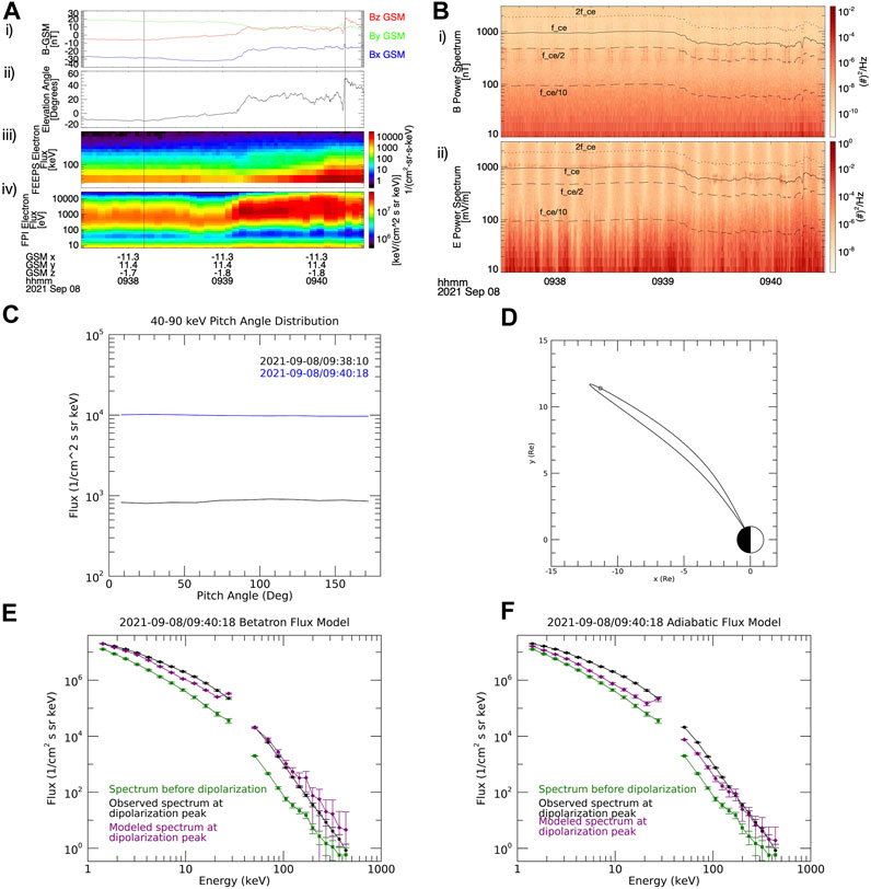
FIGURE 1. Data from MMS for the first case study event, 8 September 2021. (A-i) Magnetic field vector in GSM coordinates, (A-ii) Magnetic elevation angle, (A-iii) FEEPS energetic electron flux, (A-iv) FPI thermal electron flux, (B-i) Magnetic field power spectrum, (B-ii) Electric field power spectrum, (C) Pitch angle distributions for 40–90 keV electrons before the dipolarization (black) and at the peak of the dipolarization (blue), (D) Map of the location of MMS at the time of the observation (black circle) with the field line on which it is located as modeled using the Tsyganenko and Stern (1996) model, mapped using the IRBEM library (Boscher et al., 2004–2008), (E) Energy spectrum of observed electrons before the dipolarization (green squares), observed electrons at peak of dipolarization (black circles), and betatron model of electrons at peak (purple diamonds), (F) Energy spectrum of observed electrons before the dipolarization (green squares), observed electrons at peak of dipolarization (black circles), and adiabatic model of electrons at peak (purple diamonds). Error bars derived from Poisson statistics for particle measurements and errors from data files for field measurements.

For this event, MMS is located on the duskside of the magnetotail, slightly below the magnetic equator. There is a relatively high B_x and B_y before the dipolarization. There is a slight increase in B_z around 09:39, but the main dipolarization occurs shortly after 09:40. Following a dip in B_z, it jumps by ∼20 nT and θ increases to $>50°$. The energetic electron flux also increases ataround the same time as the dipolarization. There is some acceleration associated with the smaller dipolarization at 09:39, but most of it is associated with the main dipolarization. Because Eq. (1) is linear, we can combine the acceleration from the two dipolarizations together and use the total change in B_z and the total change in energy. The flux enhancement arrives a few seconds before the sharp dipolarization, which is similar to what is seen in other studies that used a similar methodology (e.g., Turner et al., 2016; Malykhin et al., 2018; Tang et al., 2020; Vaivads et al., 2021). However, the successive dipolarizations do present some difficulties for the model to be discussed in Section 6. There is not much wave activity visible in the magnetic field spectrum, but there is some wave activity around f_ce. The PAD is quite isotropic both before and after the dipolarization, which would not suggest betatron acceleration since it usually produces peaked PADs. However, the betatron model fluxes align very closely with the observation from ∼50–150 keV. At $<$20 keV, the model is slightly below the observation, and at $>$150 keV, the model is slightly higher than the observation, although at this point there is low enough flux that there is considerable uncertainty and we are approaching the one-count limit of the instrument. Adding in Fermi acceleration for an adiabatic model, however, decreases the modeled flux. This is because the modeled betatron acceleration was stronger than the modeled Fermi acceleration, and whereas before we were assuming all the particles underwent betatron acceleration, we are now assuming that some of the particles underwent betatron acceleration and some underwent Fermi acceleration. This means that now the model underestimates the observed flux except for at the highest energies where there is large uncertainty. A full list of all the parameters measured for this event are in Table 1.

TABLE 1

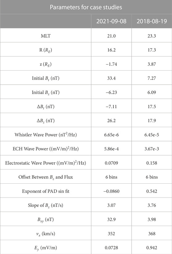
TABLE 1. Values of the parameters tested in Section 5 for the two case studies.

The second example is from 19 August 2018, around 18:22 UTC. MMS is located at a position of (−16.6, 3.0, 3.9) R_E in GSM coordinates–on the duskside of the magnetotail again but closer to midnight and above the equator this time. Figure 2 shows data for this event, similar to Figure 1 for the previous event. In this case B_x and B_y are low before the dipolarization, as is B_z. Immediately following the minimum, shortly before 18:21, there is an increase in B_z, and there are a few more bumps before the sharp increase around 18:22:10, which increases θ to nearly 90°. The bipolar B_y signature is characteristic of a flux rope, which is not unexpected since DFs can form from flux ropes (e.g., Lu et al., 2015; Vogiatzis et al., 2015). Around 18:22, energetic electron fluxes also begin to increase. There are three periods around 18:21 with electromagnetic waves in the lower band, between 0.1f_ce and 0.5f_ce in both fields, but not at the time of the main dipolarization. Throughout the time period, there are ECH waves, with the first three harmonics clearly visible in the electric field spectrum. The pitch angle distribution for 40–90 keV electrons was isotropic before the dipolarization but slightly peaked around 90° at the peak of the dipolarization, which is the expected behavior from betatron acceleration. However, the betatron acceleration model vastly overestimates observed electron flux by multiple orders of magnitude for all energies $>$2 keV (although the uncertainty is very large above 100 keV). The adiabatic model still predicts fluxes that are too high, but the error is reduced compared to the betatron model. The parameters for this example are also shown in Table 1, showing the low initial B_t, high E_y, and stronger wave power.

FIGURE 2

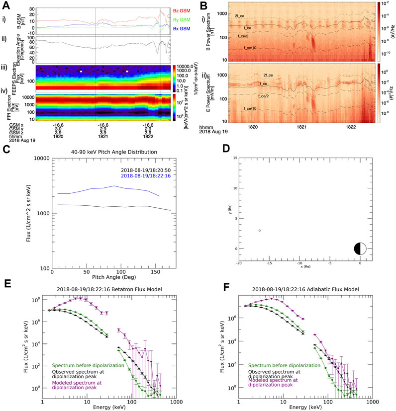
FIGURE 2. Data from MMS for the second case study event, 19 August 2018, similar to Figure 1. (A-i) Magnetic field vector in GSM coordinates, (A-ii) Magnetic elevation angle, (A-iii) FEEPS energetic electron flux, (A-iv) FPI thermal electron flux, (B-i) Magnetic field power spectrum, (B-ii) Electric field power spectrum, (C) Pitch angle distributions for 40–90 keV electrons before the dipolarization (black) and at the peak of the dipolarization (blue), (D) Map of the location of MMS at the time of the observation, mapped using the IRBEM library (Boscher et al., 2004–2008), (E) Energy spectrum of observed electrons before the dipolarization (green squares), observed electrons at peak of dipolarization (black circles), and betatron model of electrons at peak (purple diamonds), (F) Energy spectrum of observed electrons before the dipolarization (green squares), observed electrons at peak of dipolarization (black circles), and adiabatic model of electrons at peak (purple diamonds). Error bars derived from Poisson statistics for particle measurements and errors from data files for field measurements.

5 Statistical results

Statistically, we assessed how well the models performed by energy at 1.42 keV and above. We used two different methods: we compared the average ratio of the modeled flux to the observed flux (using the geometric mean to reduce the effect of outliers), and we calculated the root mean square error of the models normalized to the standard deviation. We did this for each energy channel to determine if the model worked for a certain energy range but not the entire range studied. In calculating these statistics, we excluded data points with fewer than 4 counts in the MMS data ($>50\%$ error in the observation from Poisson statistics).

5.1 Betatron model

Our first investigation was into how well purely betatron acceleration Eq. (5) describes the increase in energetic electrons at dipolarization fronts. The statistics for all events are given in the second and third columns of Table 2. This table shows that, on average, the model results are a little too high but do give an order of magnitude estimate. However, there is a very large error, suggesting that for some events the modeled flux is a large overestimate and for some it is a large underestimate. Also, between 10 and 100 keV, the energy range at which we expect the model to be most accurate, the modeled and observed flux agree within error for only about 25%–33% of the events. The same calculations were done using phase space density instead of flux and showed the same results, so the rest of the analysis for this study was done using flux to make error calculations more straightforward.

TABLE 2

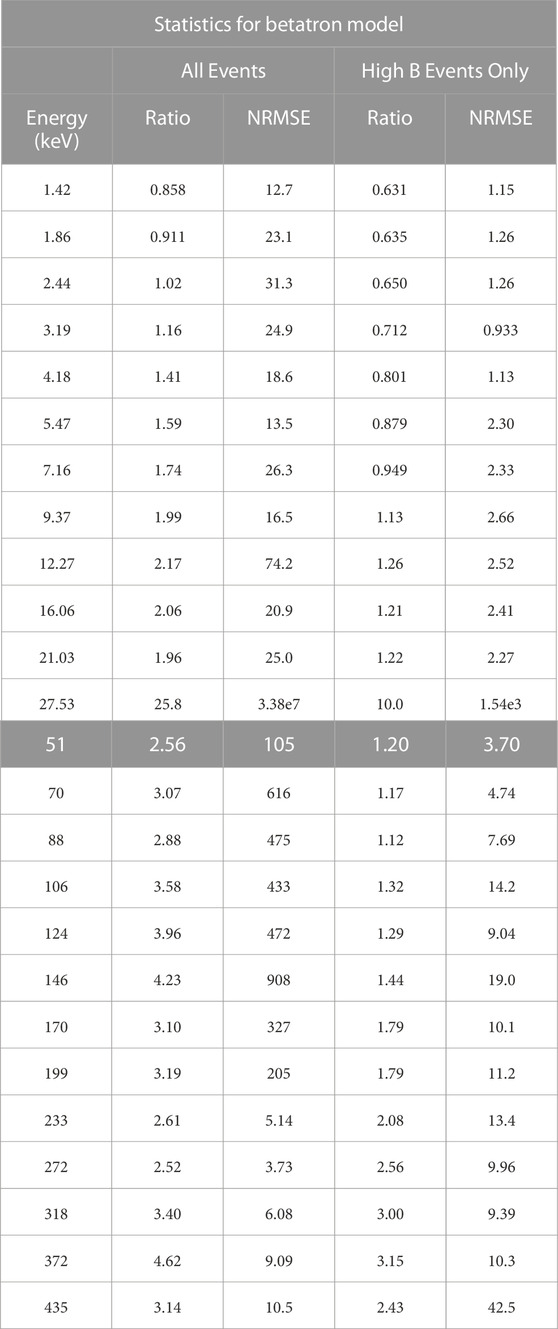
TABLE 2. Average ratio of modeled flux over observed flux and normalized root mean square error of the model for each energy channel for the betatron acceleration model. The highlighted 27.53 keV row is the energy channel at which the power law is fit across the gap between instruments, so this data point is unreliable.

Although the model was not very accurate in the aggregate, we examined several parameters to see if any of them had an effect on the accuracy. One of these parameters was the initial magnetic field. Figure 3 shows the normalized root mean square error for each event (over all energies) as a function of the initial magnetic field (panel (a)). This shows that there is a clear correlation between error and initial magnetic field, with most of the events with the highest error occurring when B_ti < 10 nT. We also broke it down by energy to ensure that the high error was not a result of the high or low energies. Panel (b) shows that at all energies, the model overestimates the observations more for events with lower B_ti. Taking this into account, we again calculated the statistics for all events, but removing all events with B_ti < 10 nT (Table 2, fourth and fifth columns). After removing the events with low initial magnetic field decreases the error for most energy channels, although the error is still high.

FIGURE 3

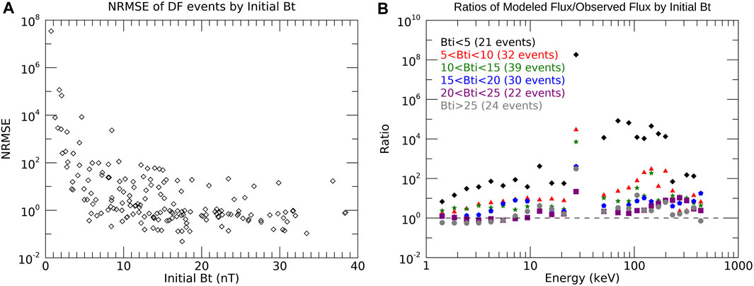
FIGURE 3. A measure of how accurate the betatron model is by initial B_t. (A) Normalized root mean square error for each event by initial B_t, (B) Average ratio of modeled flux over observed flux for each energy, binned by initial B_t. The data points at 27.53 keV are unreliable because of the transition from the FPI instrument to the FEEPS instrument.

Aside from the initial magnetic field, there were several parameters we studied that did not have similar conclusive results. First, we looked at the position of the event, by MLT, radius, and GSM z coordinate. Once again, we separated out events with low initial magnetic field. Figures 4A–C shows the normalized root mean square error for each event as a function of these parameters. We did not find any systematic relationship between any of these parameters and the accuracy of the model. We also examined other basic magnetic field values, namely, the initial B_z, the change in B_z, and the change in B_t (Figures 4D–F). None of these parameters statistically affected the model. There is potentially a correlation between highly negative initial B_z ($<-10$ nT) and higher error, but there is not a clear enough relationship to make any definitive statements. Otherwise, none of these parameters statistically affected the model.

FIGURE 4

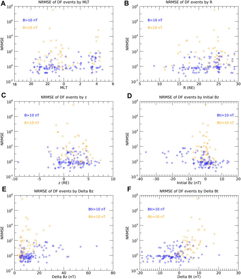
FIGURE 4. The normalized root mean square error of the betatron model for each event by different parameters related to position and magnetic field. (A) MLT, (B) R, (C) z, (D) Initial B_z, (E) ΔB_z, (F) ΔB_t. For each graph, the orange points are for events with low initial B_t ($<$10 nT) and the blue points are for events with high initial B_t ($>$10 nT).

Having studied some basic characteristics, we looked in more detail at specific parameters that could be causing the model to be inaccurate. Since we used a purely betatron acceleration model, it does not account for wave-particle interactions, so the presence of waves could introduce another process not included in our calculations. To study waves at the frequencies of interest, we need higher time resolution, so we could only use events that had burst data available. This reduced our sample size in this section to 107 events. We first studied whistler-mode waves, since they are known to be a common accelerator of energetic electrons (e.g., Demekhov et al., 2006), and have been associated with energetic electron enhancements at dipolarization fronts (Huang et al., 2012). To characterize the power of whistler waves present at the dipolarization, we measured the intensity of the magnetic field power spectrum between the electron cyclotron frequency and 0.1f_ce during the event. When looking at the wave spectra for these events, we noticed that several events had a signature consistent with electron cyclotron harmonic (ECH) waves as well, so we studied those too. We measured the intensity of the electric field power spectrum between f_ce and 1.5f_ce to find the strength of the first harmonic for each event. Finally, we looked at electrostatic waves as well since they were also a common occurrence. Unlike with whistler and ECH waves, these do not depend on characteristics of the plasma, so to find the strength of electrostatic waves we simply took the intensity of the electric power spectrum between 10 and 500 Hz, which covers the majority of the frequency range in which these waves occur. Figure 5 shows how the errors for each event depend on the intensity of these three wave modes. Once again, although waves were not included in the model, an increase in wave power from any of these modes did not meaningfully make the model less accurate. For ECH waves, Zhang and Angelopoulos (2014) found a time lag of on average ∼60 s between the DF passing and the waves occurring, so we may not be measuring the full extent of ECH waves. However, with the variable lag, multiple dipolarizations often occurring, and the limited time range of burst data, it was difficult to measure the ECH wave power more precisely.

FIGURE 5

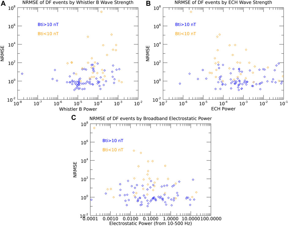
FIGURE 5. The normalized root mean square error of the betatron model applied to each event for the power of the wave modes studied. (A) Whistler-mode waves (magnetic field spectrum), (B) ECH waves, (C) Electrostatic Waves. For each graph, the orange points are for events with low initial B_t ($<$10 nT) and the blue points are for events with high initial B_t ($>$10 nT).

Finally, there are a few other miscellaneous properties that could make the betatron model inaccurate. In a superposed epoch analysis, the parameter with the largest spread aside from flux was E_y (Runov et al., 2011), so we wanted to know if there was any correlation there. As Figure 6F shows, when controlling for initial B_t, there is in fact a correlation between increased E_y and where the model overestimates the observation and has a higher error. Panel (g) shows that the increased error for higher E_y begins at around 4 keV and continues to around 200–300 keV. However, many other properties did not show any correlation. We are comparing the results of our model to the flux of electrons when B_z peaks, but in many cases, the energetic electron flux continues to increase for a few seconds after the peak of B_z, so since the model overestimates the observed flux on average, comparing the results of the model to the observed peak electron flux could be more accurate, but the events for which the electron flux and B_z peaked at the same time were no more accurate than the events that had a large offset (Figure 6A). Betatron acceleration affects electrons with perpendicular pitch angles, so if betatron acceleration is the dominant process, we expect to see PADs peaked around 90°. However, not all of the events studied showed a 90° peaked pitch angle distribution, so we might expect isotropic and field-aligned distributions to diverge from the model more. To quantify this, we fit the pitch angle distribution to a sinⁿ(α) fit and classified the distribution based on the exponent, n. We defined n < − 0.75 as strongly field-aligned, −0.75 < n < − 0.25 as weakly field-aligned, −0.25 < n < 0.25 as isotropic, 0.25 < n < 0.75 as weakly 90° peaked, and n > 0.75 as strongly 90° peaked. Once again, model performance was not correlate with PADs (Figure 6B). Unlike some other statistical studies of DFs, we did not put any restrictions on how steep the dipolarization had to be, or how quickly the peak B_z had to follow the minimum B_z beyond both occurring within the 3-min window, so this could result in some slower dipolarizations being included in our dataset. However, we did not find that the model fit the observations better when the dipolarization was steeper (Figure 6C) or when limiting our search to events that had a 4 nT increase within 6 s preceding the maximum B_z (a list of these events can be found in Supplementary Table S2). If the events are occurring far from the neutral sheet, the geometry of the event is more complicated and a simple model such as this would not necessarily work because of the larger B_x and B_y components (Tverskoy, 1969). To test if this is causing errors in the model, we also examined the model as a function of the combined x and y components of B. We again did not find any correlation between B_xy and model error when accounting for the previously-discussed effect of initial B_t (Figure 6D). We hypothesized that the speed at which the plasma flows towards Earth could affect the model, but again there was no correlation between v_x and the error of the model (Figure 6E).

FIGURE 6

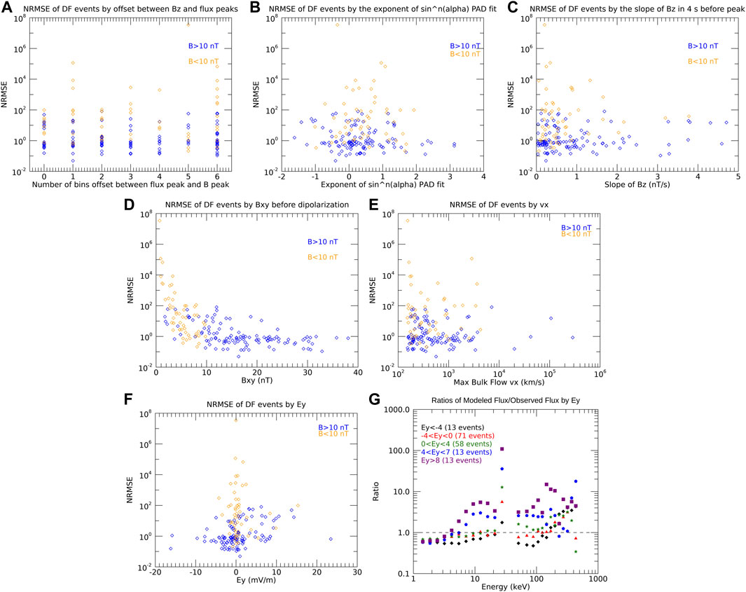
FIGURE 6. The normalized root mean square error of the betatron model applied to each event for the other parameters studied. (A) Number of bins between the B_z peak and the peak of electron flux, (B) Exponent of sinⁿ(α) fit for pitch angle distribution, (C) Slope of B_z, (D) B_xy, (E) v_x, (F) E_y, (G) Average ratio of modeled flux over observed flux for each energy, binned by E_y. For each normalized root mean square error graph, the orange points are for events with low initial B_t ($<$10 nT) and the blue points are for events with high initial B_t ($>$10 nT).

As mentioned above, this relies on a few assumptions, primarily that the phase-space density of the source population is the same as the phase-space density of the particles measured before the DF and the initial magnetic fields were the same for the source population and the measured particles. However, another potential cause of error is that betatron acceleration affects perpendicular energy but we applied it to the entire population. To test this, we used the same analysis but limited the to only particles with a perpendicular pitch angles (74°–106°). Only considering perpendicular fluxes did not meaningfully change our results, and the betatron model was not significantly more accurate when only considering perpendicular fluxes.

5.2 Adiabatic model

The betatron model did not conclusively fit the data, so next we tested an adiabatic model using Eq. (9). Fermi acceleration was generally weaker than betatron acceleration for these events, so replacing purely betatron acceleration with a mix of betatron and Fermi acceleration greatly reduced the modeled electron fluxes. Including the adiabatic model resulted in an underestimation of the observed flux (Table 3).

TABLE 3

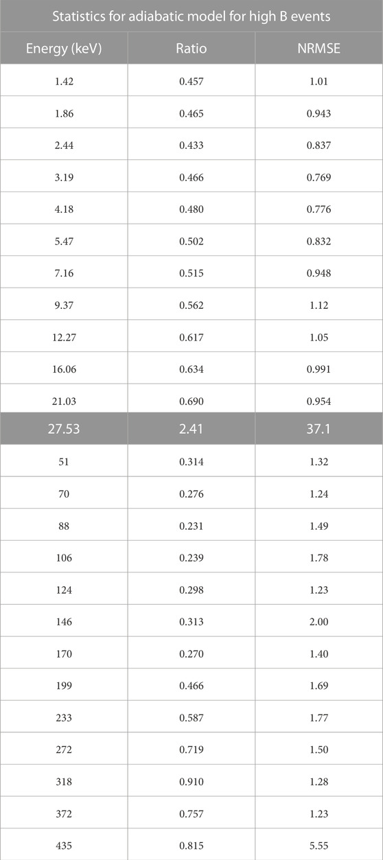
TABLE 3. Average ratio of modeled flux over observed flux and normalized root mean square error of the model for each energy channel for the adiabatic acceleration model, removing events with low initial B_t. The highlighted 27.53 keV row is the energy channel at which the power law is fit across the gap between instruments, so this data point is unreliable.

The combination of betatron and Fermi acceleration greatly reduced the error compared to the betatron-only model, but the large error indicates that this model still does not fully explain the data. It is less clear than for the betatron model, but a low initial B_t again greatly increased the error in the model, so Table 3 excludes events with initial B_t < 10 nT. Figure 7 shows the error for each event by initial B_t (panel (a)) and the ratio of the modeled flux to the observed flux for each energy as binned by initial B_t (panel (b)).

FIGURE 7

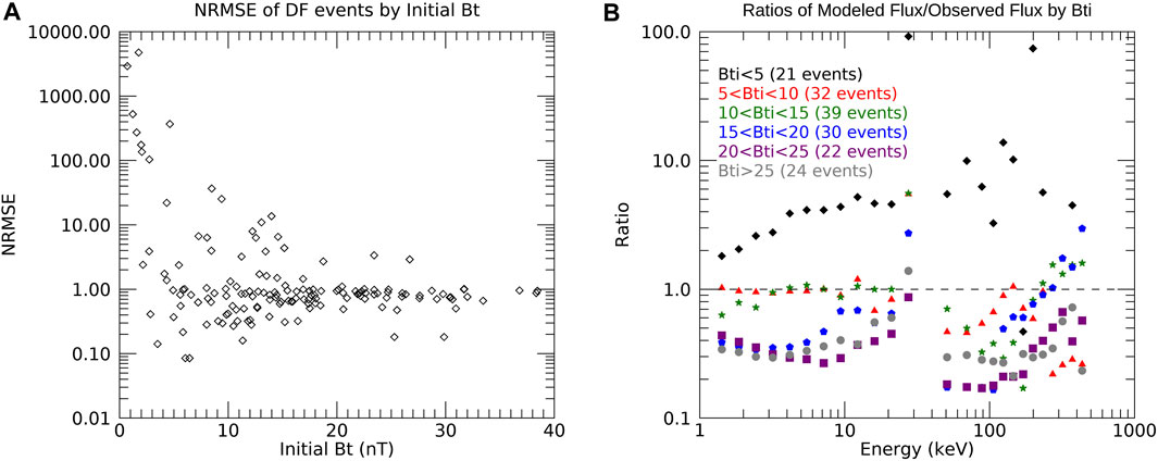
FIGURE 7. A measure of how accurate the adiabatic model is by initial B_t. (A) Normalized root mean square error for each event by initial B_t, (B) Average ratio of modeled flux over observed flux for each energy, binned by initial B_t. The data points at 27.53 keV are unreliable because of the transition from the FPI instrument to the FEEPS instrument.

As for the betatron model, we examined several parameters to determine if any of them had a major effect. The model’s error was not significantly affected by position, as shown by the errors in Figures 8A–C. It was not affected by B_zi, ΔB_t, or ΔB_z either (Figures 8D–F). Nor was there any correlation between the error of the model and strength of whistler waves, ECH waves, or electrostatic waves, as shown in Figure 9.

FIGURE 8

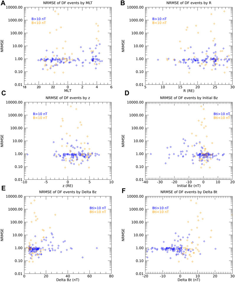
FIGURE 8. The normalized root mean square error of the adiabatic model for each event by different parameters related to position and magnetic field. (A) MLT, (B) R, (C) z, (D) Initial B_z, (E) ΔB_z, (F) ΔB_t. For each graph, the orange points are for events with low initial B_t ($<$10 nT) and the blue points are for events with high initial B_t ($>$10 nT).

FIGURE 9

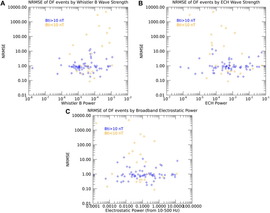
FIGURE 9. The normalized root mean square error of the adiabatic model applied to each event for the power of the wave modes studied. (A) Whistler-mode waves (magnetic field spectrum), (B) ECH waves, (C) Electrostatic Waves. For each graph, the orange points are for events with low initial B_t ($<$10 nT) and the blue points are for events with high initial B_t ($>$10 nT).

Looking at E_y, the correlation that was visible in the betatron acceleration is no longer apparent, both when looking at the error for the full event (Panel (f)) and the ratio of the modeled flux to the observed flux at each energy (Panel (g)). We also looked at the same parameters that did not affect the betatron model of the offset between B_z peak and flux peak, PAD, B_z slope, B_xy, and v_x. Again, none of these had any noticeable effect when accounting for the influence of the initial B_t (Figures 10A–E). We also compared events when betatron acceleration was stronger and events when Fermi acceleration was stronger. For most events, betatron acceleration was much stronger than Fermi acceleration, but the model had similar error for both types of events.

FIGURE 10

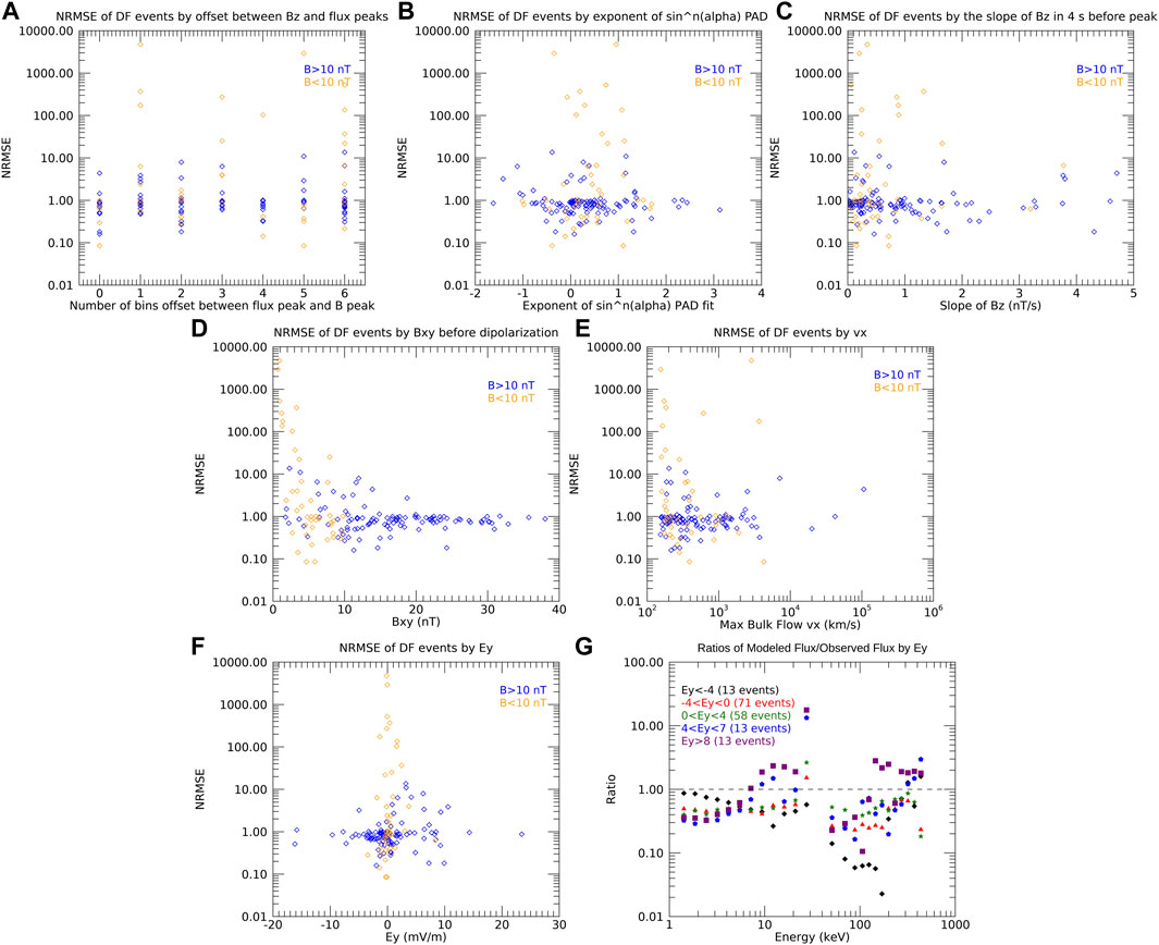
FIGURE 10. The normalized root mean square error of the adiabatic model applied to each event for the other parameters studied. (A) Number of bins between the B_z peak and the peak of electron flux, (B) Exponent of sinⁿ(α) fit for pitch angle distribution, (C) Slope of B_z, (D) B_xy, (E) v_x, (F) E_y, (G) Average ratio of modeled flux over observed flux for each energy, binned by E_y. For each normalized root mean square error graph, the orange points are for events with low initial B_t ($<$10 nT) and the blue points are for events with high initial B_t ($>$10 nT).

6 Discussion and conclusion

The two case studies demonstrate the difficulty of modeling the acceleration of electrons near dipolarization fronts. As mentioned in Section 4, the specific characteristics of Event 1 have some complications. The electrons arriving around 10 s before the dipolarization is not out of the ordinary compared to what other studies found (e.g., Turner et al., 2016; Malykhin et al., 2018; Tang et al., 2020; Vaivads et al., 2021), but it is earlier than would be expected for the fast-moving electrons. Additionally, we add the change in energy from multiple dipolarizations since the equation is linear, but since subsequent dipolarizations energize electrons at different energies (Turner et al., 2016) this simplification is only valid for a part of the energy range. Different dipolarizations may also have sources in different regions considering the localization of the structure, so using a single population as the source could be incorrect in total even if it is correct in part. Pitch angle distributions are often used to identify adiabatic acceleration mechanisms, as discussed in Section 1 (e.g., Wu et al., 2006). Although the event from 8 September 2021 (Event 1) had an isotropic distribution and the event from 8 August 2018 (Event 2) had a final distribution that was weakly peaked about 90°, it was Event 1 for which the betatron model fit well, and Event 2 that had a large error, the reverse of what the PADs would suggest. Events far from the center of the plasma sheet and with a large B_xy could violate some of the assumptions we made in deriving our equations (Tverskoy, 1969). Both case study events were fairly far away from the magnetic equator, with the closer event, Event 1, at z = −1.74 R_E in GSM coordinates, so we must be careful with our conclusions. Event 1 had a much higher B_xy than Event 2, and the betatron model still fit Event 1 better. One factor that seems to fit our initial hypotheses is that there is more wave activity in Event 2, which could explain why the model, which does not include wave-particle interactions, is less accurate for that event. This could be an explanation only if the particles are transferring energy to the waves however, and not the reverse, since the model predicts a flux that is higher than the observation. However, a confounding factor when attempting to quantify the effect of waves is that these electrons could have interacted with waves at a location away from the spacecraft and therefore waves that did not reach the spacecraft and were not observed could still affect the observed particles. While the characteristics of these two case studies do not explain how accurate the model is based on our hypotheses before we began the study, they do fit with the statistical correlations found in this investigation. The initial B_t for Event 1 is fairly large, while the initial B_t in Event 2 is much smaller, and below the 10 nT threshold we set as “low initial B_t” to separate out when calculating statistics for the other parameters. Event 2 also has a higher E_y than Event 1, which matches the correlation we found, although neither event had a very high E_y. Event 2 being a “flux-rope-type” DF could play a role in the inaccuracy of the model since electrons in this type of DF are less likely to undergo betatron acceleration than for traditional DFs (Lu et al., 2016).

Deciding when to use B_z and B_t in the model relies on assumptions about being close to the magnetic equator. However, the fact that we do not find that the model has higher error when z becomes large or when B_xy becomes large shows that these assumptions may not be the leading cause of inaccuracies in our model. In fact, the error is higher when B_xy is small, meaning that B_z and B_t are almost the same. This suggests that using ΔB_t rather than ΔB_z in our calculations would not reduce the error. If we use B_z to calculate the magnetic moment in Eq. (1) as well, then Eq. (3) becomes $W_{\perp 2}=W_{\perp 1}\frac{B_{z_2}}{B_{z_1}}$, which is the commonly used equation used for betatron acceleration in other studies (e.g., Turner et al., 2016). Although we made different assumptions for our study that produced a different form of the equation, we checked if this equation was more correct. We found that this form of the equation was in fact less accurate and also did not have a correlation with z, so using this different betatron acceleration equation is not necessarily more correct in general, even though it should be valid for a magnetotail configuration (Zelenyi et al., 2004). The Runov et al. (2013) case study found a relationship between B_xy and PADs, with primarily pancake type distributions at |B_xy| < 5 nT and primarily cigar type distributions at |B_xy| > 10 nT. If we could find this behavior in our statistical study, it could provide evidence of different acceleration methods at different locations away from the equator, but we found no difference in PADs for larger or smaller B_xy.

We were unable to find a link between wave activity and inaccuracy of the adiabatic model. A potential reason for this is that, given the nature of the study, we were unable to carefully determine which wave frequencies would have the strongest interaction with the particles in each case. As a result, some of the wave activity with high amplitudes that we measured may not have interacted with the electrons at all, in which case adiabatic processes would still dominate despite intense wave activity.

The correlations we did find were that the betatron model had a higher error when initial B_t was lower and when E_y was higher, while the adiabatic model had the same correlation with initial B_t but not E_y. In both cases, the model overestimated the observed flux. The model producing a higher error with a lower initial B_t could be because initial B_t is in the denominator of the equation, so when it is very small the equation no longer holds true. When E_y is higher, there is a higher rate of magnetic flux transport (Schödel et al., 2001), so the electrons are being transported from farther away where they are more likely to have had different initial conditions. When E_y is low, the acceleration is likely more local. However, since the E ×B drift is included in the adiabatic acceleration equation, that cause of error disappears in the adiabatic model and there is no longer a correlation with E_y. We also found that there was not a correlation between E_y and v_x, supporting the results from Runov et al. (2011) that there is no significant flux transport in the plasma flow ahead of the front. The presence of E_y suggests that the DF is not a true tangential discontinuity, which would allow particles to penetrate across the boundary. Although this is not measured in the frame of the DF, other studies have found E_y in the DF rest frame that supports the idea that there is plasma exchange across the boundary (e.g., Zhou et al., 2019).

One potential interpretation of this study is that energetic electron acceleration at DFs is only adiabatic for some events, but not in general. We found no correlation between higher error and more wave power for the modes we studied, but there could be wave-particle interactions with other modes we did not measure or other non-adiabatic processes at play. However, another explanation is that we failed to correctly identify the source electrons that are being accelerated. The electrons we identify as the source are ahead of the dipolarization, not the ones being accelerated. We can assume that the electrons we are measuring are the same as the source population if there is a relatively flat phase space density gradient in the tail. Many studies have used this approach (Asano et al., 2010; Fu et al., 2011; Turner et al., 2016; Malykhin et al., 2018; Tang et al., 2020), and it would require extremely fortuitous spacecraft locations to measure both the source and resultant populations directly, but there are problems with this approach. Fu et al. (2011) found that for certain energies, the distribution of electrons varied, causing their model to not work at those energies. This also may systematically underestimate the measured acceleration efficiency since the plasma sheet is generally hotter closer to Earth (Liu et al., 2017b). The source for the accelerated population can be as distant as the plasma sheet boundary layer or lobes, and below ∼10 keV most of the source population is from those distant regions but, However, at a few 10 s of keV, the source is mostly in the tail at a range of distances and at energies higher than a few 10 s of keV, the source is primarily within the plasma sheet, so assuming a plasma sheet source is reasonable for most of our energy range of interest (Birn et al., 2014), although there are anisotropies in different regions complicating this picture (Birn et al., 2022). The azimuthally localized nature of DFs is another factor that can negatively affect our ability to make accurate assumptions about the source population. One way of viewing DFs is as the boundary between the population of the plasma sheet and the population of a low-entropy bubble (e.g., Yang et al., 2011). In this scenario, the flat phase-space density gradient assumption is violated. The studies cited above used the same source identification method as our investigation and were able to describe electron acceleration using betatron acceleration, but they all studied just one or a few events. It is possible that identifying the source in this way works in some cases but not in general. If this is the case, more work would need to be done to determine when and why the source identification is successful beyond the correlation with parameters we found in this study.

We have conducted a large survey of 168 dipolarization events with coincident energetic electron acceleration. We tested a betatron acceleration model and an adiabatic acceleration model with specific assumptions about the particle source and magnetic field and found that neither fit the observed data for the statistical sample. They key results were:

- The betatron model overestimates the observed flux with a large error

- The adiabatic model underestimates the observed flux with a slightly smaller error than the betatron model

- Several parameters tested, only correlations were higher error with lower initial B_t (both models) and higher error with large E_y (betatron model only)

These results could show that either adiabatic acceleration alone is not enough to explain electron acceleration at dipolarization fronts and other factors need to be included, or that assuming the source population is the same as the quiet population ahead of the front is not generally accurate.

Data availability statement

Publicly available datasets were analyzed in this study. This data can be found here: https://lasp.colorado.edu/mms/sdc.

Author contributions

SC: Writing–original draft. AJ: Writing–review and editing. DT: Writing–review and editing. CG: Writing–review and editing. IC: Writing–review and editing. DB: Writing–review and editing. BM: Writing–review and editing. TL: Writing–review and editing. JB: Writing–review and editing. JF: Writing–review and editing.

Funding

The author(s) declare financial support was received for the research, authorship, and/or publication of this article. This work was supported by funding from the MMS mission, under NASA contracts NNG04EB99C and 80NSSC20K1790.

Acknowledgments

The authors would like to acknowledge FD. Wilder for his help in calculating magnetic field gradients from MMS data. We acknowledge the use of the IRBEM library, the latest version of which can be found at https://doi.org/10.5281/zenodo.6867552.

Conflict of interest

Authors CG, JB, and JF were employed by The Aerospace Corporation.

The remaining authors declare that the research was conducted in the absence of any commercial or financial relationships that could be construed as a potential conflict of interest.

Publisher’s note

All claims expressed in this article are solely those of the authors and do not necessarily represent those of their affiliated organizations, or those of the publisher, the editors and the reviewers. Any product that may be evaluated in this article, or claim that may be made by its manufacturer, is not guaranteed or endorsed by the publisher.

Supplementary material

The Supplementary Material for this article can be found online at: https://www.frontiersin.org/articles/10.3389/fspas.2023.1266412/full#supplementary-material

Footnotes

¹For 2022, only May 1-October 1 is covered because the survey took place before 31 October 2022 and the orbit of MMS has evolved such that the tail season ends earlier in later years.

References

Angelopoulos, V., Baumjohann, W., Kennel, C., Coroniti, F. V., Kivelson, M., Pellat, R., et al. (1992). Bursty bulk flows in the inner central plasma sheet. J. Geophys. Res. Space Phys. 97, 4027–4039. doi:10.1029/91ja02701

CrossRef Full Text | Google Scholar

Arnold, H., Drake, J. F., Swisdak, M., Guo, F., Dahlin, J. T., Chen, B., et al. (2021). Electron acceleration during macroscale magnetic reconnection. Phys. Rev. Lett. 126, 135101. doi:10.1103/physrevlett.126.135101

PubMed Abstract | CrossRef Full Text | Google Scholar

Asano, Y., Shinohara, I., Retinò, A., Daly, P., Kronberg, E., Takada, T., et al. (2010). Electron acceleration signatures in the magnetotail associated with substorms. J. Geophys. Res. Space Phys., 115. doi:10.1029/2009ja014587

CrossRef Full Text | Google Scholar

Baumjohann, W., Hesse, M., Kokubun, S., Mukai, T., Nagai, T., and Petrukovich, A. (1999). Substorm dipolarization and recovery. J. Geophys. Res. Space Phys. 104, 24995–25000. doi:10.1029/1999ja900282

CrossRef Full Text | Google Scholar

Birn, J., Hesse, M., Nakamura, R., and Zaharia, S. (2013). Particle acceleration in dipolarization events. J. Geophys. Res. Space Phys. 118, 1960–1971. doi:10.1002/jgra.50132

CrossRef Full Text | Google Scholar

Birn, J., Hesse, M., and Runov, A. (2022). Electron anisotropies in magnetotail dipolarization events. Front. Astronomy Space Sci. 9, 908730. doi:10.3389/fspas.2022.908730

CrossRef Full Text | Google Scholar

Birn, J., Runov, A., and Hesse, M. (2014). Energetic electrons in dipolarization events: spatial properties and anisotropy. J. Geophys. Res. Space Phys. 119, 3604–3616. doi:10.1002/2013ja019738

CrossRef Full Text | Google Scholar

Blake, J., Mauk, B., Baker, D., Carranza, P., Clemmons, J., Craft, J., et al. (2016). The fly’s eye energetic particle spectrometer (feeps) sensors for the magnetospheric multiscale (mms) mission. Space Sci. Rev. 199, 309–329. doi:10.1007/s11214-015-0163-x

CrossRef Full Text | Google Scholar

Boscher, D., Bourdarie, S., O’Brien, P., and Guild, T. (2004-2008). IRBEM library V4.3.

Google Scholar

Burch, J., Moore, T., Torbert, R., and Giles, B. (2016). Magnetospheric multiscale overview and science objectives. Space Sci. Rev. 199, 5–21. doi:10.1007/s11214-015-0164-9

CrossRef Full Text | Google Scholar

Chen, G., Fu, H., Zhang, Y., Su, Z., Liu, N., Chen, L., et al. (2021). An unexpected whistler wave generation around dipolarization front. J. Geophys. Res. Space Phys. 126, e2020JA028957. doi:10.1029/2020ja028957

CrossRef Full Text | Google Scholar

Demekhov, A., Trakhtengerts, V. Y., Rycroft, M., and Nunn, D. (2006). Electron acceleration in the magnetosphere by whistler-mode waves of varying frequency. Geomagnetism Aeronomy 46, 711–716. doi:10.1134/s0016793206060053

CrossRef Full Text | Google Scholar

Drake, J., Swisdak, M., Che, H., and Shay, M. (2006). Electron acceleration from contracting magnetic islands during reconnection. Nature 443, 553–556. doi:10.1038/nature05116

PubMed Abstract | CrossRef Full Text | Google Scholar

Ergun, R., Ahmadi, N., Kromyda, L., Schwartz, S., Chasapis, A., Hoilijoki, S., et al. (2020a). Observations of particle acceleration in magnetic reconnection–driven turbulence. Astrophysical J. 898, 154. doi:10.3847/1538-4357/ab9ab6

CrossRef Full Text | Google Scholar

Ergun, R., Ahmadi, N., Kromyda, L., Schwartz, S., Chasapis, A., Hoilijoki, S., et al. (2020b). Particle acceleration in strong turbulence in the earth’s magnetotail. Astrophysical J. 898, 153. doi:10.3847/1538-4357/ab9ab5

CrossRef Full Text | Google Scholar

Ergun, R., Tucker, S., Westfall, J., Goodrich, K., Malaspina, D., Summers, D., et al. (2016). The axial double probe and fields signal processing for the mms mission. Space Sci. Rev. 199, 167–188. doi:10.1007/s11214-014-0115-x

CrossRef Full Text | Google Scholar

Fu, H., Grigorenko, E. E., Gabrielse, C., Liu, C., Lu, S., Hwang, K., et al. (2020). Magnetotail dipolarization fronts and particle acceleration: a review. Sci. China Earth Sci. 63, 235–256. doi:10.1007/s11430-019-9551-y

CrossRef Full Text | Google Scholar

Fu, H., Khotyaintsev, Y. V., Vaivads, A., André, M., and Huang, S. (2012a). Occurrence rate of earthward-propagating dipolarization fronts. Geophys. Res. Lett., 39. doi:10.1029/2012gl051784

CrossRef Full Text | Google Scholar

Fu, H. S., Khotyaintsev, Y. V., André, M., and Vaivads, A. (2011). Fermi and betatron acceleration of suprathermal electrons behind dipolarization fronts. Geophys. Res. Lett., 38. doi:10.1029/2011gl048528

CrossRef Full Text | Google Scholar

Fu, H. S., Khotyaintsev, Y. V., Vaivads, A., André, M., and Huang, S. (2012b). Electric structure of dipolarization front at sub-proton scale. Geophys. Res. Lett., 39. doi:10.1029/2012gl051274

CrossRef Full Text | Google Scholar

Fu, W., Fu, H., Cao, J., Yu, Y., Chen, Z., and Xu, Y. (2022). Formation of rolling-pin distribution of suprathermal electrons behind dipolarization fronts. J. Geophys. Res. Space Phys. 127, e2021JA029642. doi:10.1029/2021ja029642

CrossRef Full Text | Google Scholar

Fuselier, S., Lewis, W., Schiff, C., Ergun, R., Burch, J., Petrinec, S., et al. (2016). Magnetospheric multiscale science mission profile and operations. Space Sci. Rev. 199, 77–103. doi:10.1007/s11214-014-0087-x

CrossRef Full Text | Google Scholar

Gabrielse, C., Angelopoulos, V., Runov, A., and Turner, D. L. (2014). Statistical characteristics of particle injections throughout the equatorial magnetotail. J. Geophys. Res. Space Phys. 119, 2512–2535. doi:10.1002/2013ja019638

CrossRef Full Text | Google Scholar

Grigorenko, E., Malykhin, A. Y., Shklyar, D., Fadanelli, S., Lavraud, B., Panov, E., et al. (2020). Investigation of electron distribution functions associated with whistler waves at dipolarization fronts in the earth’s magnetotail: mms observations. J. Geophys. Res. Space Phys. 125, e2020JA028268. doi:10.1029/2020ja028268

CrossRef Full Text | Google Scholar

Grigorenko, E. E., Malykhin, A. Y., Kronberg, E. A., and Panov, E. V. (2023). Quasi-parallel whistler waves and their interaction with resonant electrons during high-velocity bulk flows in the earth’s magnetotail. Astrophysical J. 943, 169. doi:10.3847/1538-4357/acaf52

CrossRef Full Text | Google Scholar

Huang, S., Zhou, M., Deng, X., Yuan, Z., Pang, Y., Wei, Q., et al. (2012). “Kinetic structure and wave properties associated with sharp dipolarization front observed by cluster,” in Annales geophysicae (Germany: Copernicus Publications Göttingen), 30, 97–107.

CrossRef Full Text | Google Scholar

Hwang, K.-J., Goldstein, M. L., Lee, E., and Pickett, J. S. (2011). Cluster observations of multiple dipolarization fronts. J. Geophys. Res. Space Phys., 116. doi:10.1029/2010ja015742

CrossRef Full Text | Google Scholar

Khotyaintsev, Y. V., Cully, C., Vaivads, A., André, M., and Owen, C. (2011). Plasma jet braking: energy dissipation and nonadiabatic electrons. Phys. Rev. Lett. 106, 165001. doi:10.1103/physrevlett.106.165001

PubMed Abstract | CrossRef Full Text | Google Scholar

Le Contel, O., Leroy, P., Roux, A., Coillot, C., Alison, D., Bouabdellah, A., et al. (2016). The search-coil magnetometer for mms. Space Sci. Rev. 199, 257–282. doi:10.1007/s11214-014-0096-9

CrossRef Full Text | Google Scholar

Lindqvist, P.-A., Olsson, G., Torbert, R., King, B., Granoff, M., Rau, D., et al. (2016). The spin-plane double probe electric field instrument for mms. Space Sci. Rev. 199, 137–165. doi:10.1007/s11214-014-0116-9

CrossRef Full Text | Google Scholar

Liu, C., Fu, H., Xu, Y., Cao, J., and Liu, W. (2017a). Explaining the rolling-pin distribution of suprathermal electrons behind dipolarization fronts. Geophys. Res. Lett. 44, 6492–6499. doi:10.1002/2017gl074029

CrossRef Full Text | Google Scholar

Liu, C., Fu, H., Xu, Y., Wang, T., Cao, J., Sun, X., et al. (2017b). Suprathermal electron acceleration in the near-earth flow rebounce region. J. Geophys. Res. Space Phys. 122, 594–604. doi:10.1002/2016ja023437

CrossRef Full Text | Google Scholar

Liu, J., Angelopoulos, V., Runov, A., and Zhou, X.-Z. (2013). On the current sheets surrounding dipolarizing flux bundles in the magnetotail: the case for wedgelets. J. Geophys. Res. Space Phys. 118, 2000–2020. doi:10.1002/jgra.50092

CrossRef Full Text | Google Scholar

Liu, J., Angelopoulos, V., Zhou, X.-Z., and Runov, A. (2014). Magnetic flux transport by dipolarizing flux bundles. J. Geophys. Res. Space Phys. 119, 909–926. doi:10.1002/2013ja019395

CrossRef Full Text | Google Scholar

Lu, S., Angelopoulos, V., and Fu, H. (2016). Suprathermal particle energization in dipolarization fronts: particle-in-cell simulations. J. Geophys. Res. Space Phys. 121, 9483–9500. doi:10.1002/2016ja022815

CrossRef Full Text | Google Scholar

Lu, S., Lu, Q., Lin, Y., Wang, X., Ge, Y., Wang, R., et al. (2015). Dipolarization fronts as earthward propagating flux ropes: a three-dimensional global hybrid simulation. J. Geophys. Res. Space Phys. 120, 6286–6300. doi:10.1002/2015ja021213

CrossRef Full Text | Google Scholar

Ma, W., Zhou, M., Zhong, Z., and Deng, X. (2020). Electron acceleration rate at dipolarization fronts. Astrophysical J. 903, 84. doi:10.3847/1538-4357/abb8cc

CrossRef Full Text | Google Scholar

Malykhin, A. Y., Grigorenko, E., Kronberg, E. A., and Daly, P. W. (2018). The effect of the betatron mechanism on the dynamics of superthermal electron fluxes within dipolizations in the magnetotail. Geomagnetism Aeronomy 58, 744–752. doi:10.1134/s0016793218060099

CrossRef Full Text | Google Scholar

Mauk, B., Blake, J., Baker, D., Clemmons, J., Reeves, G., Spence, H. E., et al. (2016). The energetic particle detector (epd) investigation and the energetic ion spectrometer (eis) for the magnetospheric multiscale (mms) mission. Space Sci. Rev. 199, 471–514. doi:10.1007/s11214-014-0055-5

CrossRef Full Text | Google Scholar

Nakamura, R., Baumjohann, W., Klecker, B., Bogdanova, Y., Balogh, A., Rème, H., et al. (2002). Motion of the dipolarization front during a flow burst event observed by cluster. Geophys. Res. Lett. 29, 3–4. doi:10.1029/2002gl015763

CrossRef Full Text | Google Scholar

Nakamura, R., Baumjohann, W., Mouikis, C., Kistler, L., Runov, A., Volwerk, M., et al. (2004). Spatial scale of high-speed flows in the plasma sheet observed by cluster. Geophys. Res. Lett. 31. doi:10.1029/2004gl019558

CrossRef Full Text | Google Scholar

Northrop, T. G. (1963). Adiabatic charged-particle motion. Rev. Geophys. 1, 283–304. doi:10.1029/rg001i003p00283

CrossRef Full Text | Google Scholar

Pan, Q., Ashour-Abdalla, M., El-Alaoui, M., Walker, R. J., and Goldstein, M. L. (2012). Adiabatic acceleration of suprathermal electrons associated with dipolarization fronts. J. Geophys. Res. Space Phys., 117. doi:10.1029/2012ja018156

CrossRef Full Text | Google Scholar

Pollock, C., Moore, T., Jacques, A., Burch, J., Gliese, U., Saito, Y., et al. (2016). Fast plasma investigation for magnetospheric multiscale. Space Sci. Rev. 199, 331–406. doi:10.1007/s11214-016-0245-4

CrossRef Full Text | Google Scholar

Runov, A., Angelopoulos, V., Gabrielse, C., Zhou, X.-Z., Turner, D., and Plaschke, F. (2013). Electron fluxes and pitch-angle distributions at dipolarization fronts: themis multipoint observations. J. Geophys. Res. Space Phys. 118, 744–755. doi:10.1002/jgra.50121

CrossRef Full Text | Google Scholar

Runov, A., Angelopoulos, V., Sitnov, M., Sergeev, V., Bonnell, J., McFadden, J., et al. (2009). Themis observations of an earthward-propagating dipolarization front. Geophys. Res. Lett. 36, L14106. doi:10.1029/2009gl038980

CrossRef Full Text | Google Scholar

Runov, A., Angelopoulos, V., Zhou, X.-Z., Zhang, X.-J., Li, S., Plaschke, F., et al. (2011). A themis multicase study of dipolarization fronts in the magnetotail plasma sheet. J. Geophys. Res. Space Phys., 116. doi:10.1029/2010ja016316

CrossRef Full Text | Google Scholar

Russell, C., Anderson, B., Baumjohann, W., Bromund, K., Dearborn, D., Fischer, D., et al. (2016a). The magnetospheric multiscale magnetometers. Space Sci. Rev. 199, 189–256. doi:10.1007/s11214-014-0057-3

CrossRef Full Text | Google Scholar

Russell, C., and McPherron, R. (1973). The magnetotail and substorms. Space Sci. Rev. 15, 205–266. doi:10.1007/bf00169321

CrossRef Full Text | Google Scholar

Russell, C. T., Luhmann, J. G., and Strangeway, R. J. (2016b). Space physics: an introduction. Cambridge University Press.

Google Scholar

Schmid, D., Nakamura, R., Volwerk, M., Plaschke, F., Narita, Y., Baumjohann, W., et al. (2016). A comparative study of dipolarization fronts at mms and cluster. Geophys. Res. Lett. 43, 6012–6019. doi:10.1002/2016gl069520

PubMed Abstract | CrossRef Full Text | Google Scholar

Schmid, D., Volwerk, M., Nakamura, R., Baumjohann, W., and Heyn, M. (2011). “A statistical and event study of magnetotail dipolarization fronts,” in Annales geophysicae (Germany: Copernicus Publications Göttingen), 29, 1537–1547.

CrossRef Full Text | Google Scholar

Schmid, D., Volwerk, M., Plaschke, F., Nakamura, R., Baumjohann, W., Wang, G., et al. (2019). A statistical study on the properties of dips ahead of dipolarization fronts observed by mms. J. Geophys. Res. Space Phys. 124, 139–150. doi:10.1029/2018ja026062

CrossRef Full Text | Google Scholar

Schödel, R., Baumjohann, W., Nakamura, R., Sergeev, V., and Mukai, T. (2001). Rapid flux transport in the central plasma sheet. J. Geophys. Res. Space Phys. 106, 301–313. doi:10.1029/2000ja900139

CrossRef Full Text | Google Scholar

Sergeev, V., Angelopoulos, V., Apatenkov, S., Bonnell, J., Ergun, R., Nakamura, R., et al. (2009). Kinetic structure of the sharp injection/dipolarization front in the flow-braking region. Geophys. Res. Lett. 36, L21105. doi:10.1029/2009gl040658

CrossRef Full Text | Google Scholar

Sergeev, V., Angelopoulos, V., Gosling, J., Cattell, C., and Russell, C. (1996). Detection of localized, plasma-depleted flux tubes or bubbles in the midtail plasma sheet. J. Geophys. Res. Space Phys. 101, 10817–10826. doi:10.1029/96ja00460

CrossRef Full Text | Google Scholar

Shklyar, D. (2017). Energy transfer from lower energy to higher-energy electrons mediated by whistler waves in the radiation belts. J. Geophys. Res. Space Phys. 122, 640–655. doi:10.1002/2016ja023263

CrossRef Full Text | Google Scholar

Smets, R., Delcourt, D., Sauvaud, J., and Koperski, P. (1999). Electron pitch angle distributions following the dipolarization phase of a substorm: interball-tail observations and modeling. J. Geophys. Res. Space Phys. 104, 14571–14581. doi:10.1029/1998ja900162

CrossRef Full Text | Google Scholar

Tang, C., Wang, X., and Zhou, M. (2020). Electron pitch angle distributions around dipolarization fronts at the off magnetic equator. J. Geophys. Res. Space Phys. 125, e2020JA028787. doi:10.1029/2020JA028787

CrossRef Full Text | Google Scholar

Torbert, R., Russell, C., Magnes, W., Ergun, R., Lindqvist, P.-A., LeContel, O., et al. (2016). The fields instrument suite on mms: scientific objectives, measurements, and data products. Space Sci. Rev. 199, 105–135. doi:10.1007/s11214-014-0109-8

CrossRef Full Text | Google Scholar

Tsyganenko, N. A., and Stern, D. P. (1996). Modeling the global magnetic field of the large-scale birkeland current systems. J. Geophys. Res. Space Phys. 101, 27187–27198. doi:10.1029/96ja02735

CrossRef Full Text | Google Scholar

Turner, D. L., Cohen, I. J., Michael, A., Sorathia, K., Merkin, S., Mauk, B. H., et al. (2021). Can earth’s magnetotail plasma sheet produce a source of relativistic electrons for the radiation belts? Geophys. Res. Lett. 48, e2021GL095495. doi:10.1029/2021gl095495

CrossRef Full Text | Google Scholar

Turner, D. L., Fennell, J., Blake, J., Clemmons, J., Mauk, B., Cohen, I., et al. (2016). Energy limits of electron acceleration in the plasma sheet during substorms: a case study with the magnetospheric multiscale (mms) mission. Geophys. Res. Lett. 43, 7785–7794. doi:10.1002/2016gl069691

CrossRef Full Text | Google Scholar

Tverskoy, B. (1969). Main mechanisms in the formation of the earth’s radiation belts. Rev. Geophys. 7, 219–231. doi:10.1029/rg007i001p00219

CrossRef Full Text | Google Scholar

Vaivads, A., Khotyaintsev, Y. V., Retino, A., Fu, H., Kronberg, E., and Daly, P. W. (2021). Cluster observations of energetic electron acceleration within earthward reconnection jet and associated magnetic flux rope. J. Geophys. Res. Space Phys. 126, e2021JA029545. doi:10.1029/2021ja029545

CrossRef Full Text | Google Scholar

Viberg, H., Khotyaintsev, Y. V., Vaivads, A., André, M., Fu, H., and Cornilleau-Wehrlin, N. (2014). Whistler mode waves at magnetotail dipolarization fronts. J. Geophys. Res. Space Phys. 119, 2605–2611. doi:10.1002/2014ja019892

CrossRef Full Text | Google Scholar

Vogiatzis, I., Isavnin, A., Zong, Q.-G., Sarris, E., Lu, S., and Tian, A. (2015). “Dipolarization fronts in the near-earth space and substorm dynamics,” in Annales geophysicae (Germany: Copernicus GmbH Göttingen), 33, 63–74.

CrossRef Full Text | Google Scholar

Williams, D., Mitchell, D., Huang, C., Frank, L., and Russell, C. (1990). Particle acceleration during substorm growth and onset. Geophys. Res. Lett. 17, 587–590. doi:10.1029/gl017i005p00587

CrossRef Full Text | Google Scholar

Wu, M., Lu, Q., Volwerk, M., Voeroes, Z., Zhang, T., Shan, L., et al. (2013). A statistical study of electron acceleration behind the dipolarization fronts in the magnetotail. J. Geophys. Res. Space Phys. 118, 4804–4810. doi:10.1002/jgra.50456

CrossRef Full Text | Google Scholar

Wu, P., Fritz, T., Larvaud, B., and Lucek, E. (2006). Substorm associated magnetotail energetic electrons pitch angle evolutions and flow reversals: cluster observation. Geophys. Res. Lett. 33, L17101. doi:10.1029/2006gl026595

CrossRef Full Text | Google Scholar

Xiao, S., Zhang, T., Wang, G., Volwerk, M., Ge, Y., Schmid, D., et al. (2017). “Occurrence rate of dipolarization fronts in the plasma sheet: cluster observations,” in Annales geophysicae (Germany: Copernicus Publications Göttingen), 35, 1015–1022.

CrossRef Full Text | Google Scholar

Yang, J., Toffoletto, F., Wolf, R., and Sazykin, S. (2011). Rcm-e simulation of ion acceleration during an idealized plasma sheet bubble injection. J. Geophys. Res. Space Phys., 116. doi:10.1029/2010ja016346

CrossRef Full Text | Google Scholar

Zelenyi, L., Malova, H., Popov, V. Y., Delcourt, D., and Sharma, A. (2004). Nonlinear equilibrium structure of thin currents sheets: influence of electron pressure anisotropy. Nonlinear Process. Geophys. 11, 579–587. doi:10.5194/npg-11-579-2004

CrossRef Full Text | Google Scholar

Zhang, X., and Angelopoulos, V. (2014). On the relationship of electrostatic cyclotron harmonic emissions with electron injections and dipolarization fronts. J. Geophys. Res. Space Phys. 119, 2536–2549. doi:10.1002/2013ja019540

CrossRef Full Text | Google Scholar

Zhang, X., Angelopoulos, V., Artemyev, A., and Liu, J. (2018). Whistler and electron firehose instability control of electron distributions in and around dipolarizing flux bundles. Geophys. Res. Lett. 45, 9380–9389. doi:10.1029/2018gl079613

CrossRef Full Text | Google Scholar

Zhou, M., Ashour-Abdalla, M., Deng, X., Schriver, D., El-Alaoui, M., and Pang, Y. (2009). Themis observation of multiple dipolarization fronts and associated wave characteristics in the near-earth magnetotail. Geophys. Res. Lett. 36, L20107. doi:10.1029/2009gl040663

CrossRef Full Text | Google Scholar

Zhou, X.-Z., Xu, Y., Runov, A., Liu, J., Artemyev, A. V., Angelopoulos, V., et al. (2019). On the origin of perpendicular ion anisotropy inside dipolarizing flux bundles. J. Geophys. Res. Space Phys. 124, 4009–4021. doi:10.1029/2019ja026519

CrossRef Full Text | Google Scholar