 Katharina N. Maetschke
 Elena A. Kronberg
 Noora Partamies
 Elena E. Grigorenko
- 1Department of Earth and Environmental Sciences, Ludwig-Maximilians-Universität München, Munich, Germany
- 2Department of Arctic Geophysics, University Centre in Svalbard (UNIS), Longyearbyen, Norway
- 3Space Research Institute, Russian Academy of Sciences, Moscow, Russia
- 4Moscow Institute of Physics and Technology, Moscow, Russia
The generation process of auroral spirals is described by different theories varying for their morphology and surrounding conditions. Here, a possible mechanism is proposed for an eastward moving auroral spiral, which was observed in Tromsø, Norway, during the expansion phase of a substorm on 18 September 2013. Measurements from the THEMIS-A and Cluster spacecraft were analyzed, which were located up to ∼10 RE duskward from the spiral generator region in the magnetosphere. Precursory to the spiral observation, concurrent magnetic field dipolarizations, flow bursts and electron injections were measured by the Cluster satellites between 13.6 and 14.2 RE radial distance from Earth. A local Kelvin-Helmholtz-like vortex street in the magnetic field was detected at the same time, which was likely caused by bursty bulk flows. The vortex street was oriented approximately in the X-Y (GSE) plane and presumably propagated towards the source region of the spiral due to a high dawnward velocity component in the flow bursts. The observations suggest that the spiral can have been generated by an associated vortex in the magnetotail and then mapped along the magnetic field lines to the ionosphere. To better understand the role of the ionosphere in auroral spiral generation, in future more mesoscale observations are required.
1 Introduction
As the optical manifestation of atmospheric ionization through precipitating electrons from the magnetosphere, auroral arcs are commonly observed as narrow bands in the nightside auroral oval. They can, however, reshape and distort into numerous small- and meso-scale structures, among those auroral spirals (Paschmann et al., 2003). An auroral spiral can occur as an individual structure or in a vortex street with multiple spirals (Hallinan, 1976). On average they have diameters of 25–75 km (Partamies et al., 2001b), but can reach sizes up to 1,300 km and thereby they are the largest vortical forms found in an auroral arc (Davis and Hallinan, 1976). As stated by Partamies et al. (2001b), spirals develop primarily during quiet magnetospheric conditions. In the course of a substorm, they occur mainly during the expansion and beginning of the recovery phase (Hallinan, 1976).
Partamies et al. (2001b) observed that the drift motion of auroral spirals coincides with the direction of the ionospheric convection. As viewed from above in the northern hemisphere, auroral spirals wind in a counterclockwise direction around upward field-aligned currents (FACs). Increased auroral precipitation in the FACs connected to brighter aurora is correlated with the winding of the spiral, while its brightness decreases with unwinding (Partamies et al., 2001b). Instead of unwinding, spirals can also decay into patchy auroral structures (Davis and Hallinan, 1976). While the auroral spiral was subject to several ground observations (Davis and Hallinan, 1976; Partamies et al., 2001b) and theoretical approaches (Hallinan, 1976; Partamies et al., 2001a), correlated space and ground measurements as performed by Keiling et al. (2009b) have rarely been done. This is due to a lack of events during which satellites were positioned in a magnetospheric region conjunct by magnetic field lines with the region of a spiral observation. Therefore, the exact generation mechanism and location, which may also vary for different magnetospheric states, is not yet established. In this paper we study an eastward moving spiral event with space measurements and propose a spiral generation mechanism following from the theory by Keiling et al. (2009b).
2 Observations
2.1 Ground-based
2.1.1 Auroral spiral
At 22:58 UT on 18 September 2013, an auroral spiral (see Figure 1 22:58 UT) was observed in Tromsø, Norway (67.176° and 115.627° geomagnetic latitude and longitude). The auroral arc along with the spiral was moving approximately towards east (see Figure 1) with the spiral itself exhibiting anti-clockwise rotation. The sense of rotation here is defined as viewed from above. From Figure 1 22:58 UT, the spiral was estimated to have a diameter of approximately 189 ± 45 km. This estimation was made by determining the zenith angle for the far (72 ± 3°) and near end (50 ± 2°) of the spiral by comparing the positions of star constellations in the photograph with the astronomy software Stellarium (Version 23.2, Zotti et al. (2021)). These angles were then used for trigonometric calculations, taking the auroral spiral to be in an approximate height of 100 km and thus reaching a diameter value of 189 ± 45 km. The spiral was observed during the expansion phase of a substorm. The onset of this substorm was taking place at approximately 22:20 UT, marked by a sharp growth of the AE index to values of ∼500 nT. The expansion phase lasted until about 23:40 UT, when the IMF turned from an entirely southward orientation to exhibiting northward peaks and the AE index decreased rapidly. No records of the duration of the spiral display or its development and decay could be obtained. At 23:27 and 23:34 UT, the photographs in Figure 1 show east-west aligned decreasing auroral activity coinciding with the end of the expansion phase.
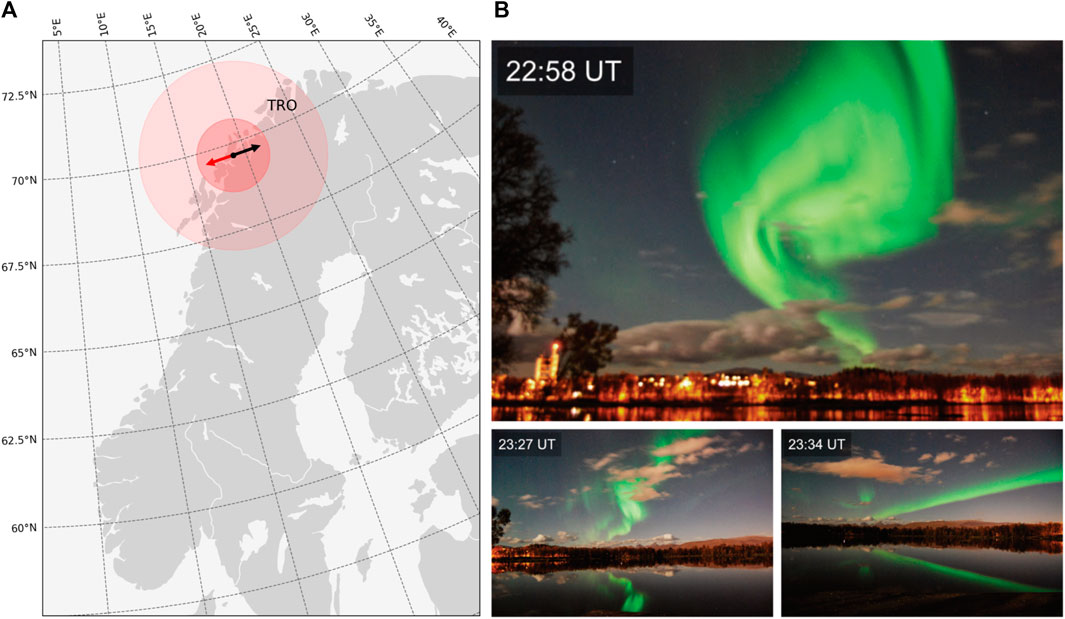
FIGURE 1. (A) Map showing the location of the spiral observation with the red circles marking the field of view from Tromsø with zenith angles of 50° and 72° mapped to an altitude of 100 km. The approximate line of sight is shown by the red arrow, while the direction of auroral movement is marked with the black arrow. The map was made using cartopy (Met Office, 2010 - 2015). (B) Photographs of the aurora taken in Tromsø on 18 September 2013 (E. Kronberg, personal communication, 22 March 2021). 22:58 UT: Auroral spiral formation. 23:27 UT and 23:34 UT: decreasing auroral activity with increasingly quiet auroral arcs.
2.1.2 Equivalent ionospheric currents
Equivalent ionospheric currents (Jeq) here are defined as sheet currents that generate magnetic field variations at the Earth’s surface that are equivalent to the measured ground horizontal field perturbations (Untiedt and Baumjohann, 1993). With the simplified assumptions that the currents flow near the Earth’s surface, approximated as a plane, the equivalent ionospheric currents can be defined as
Jeq directions as seen in Figure 2 were retrieved from 10 s IMAGE magnetometer data by the Spherical Elementary Current System (SECS) method as described by Juusola et al. (2016). Three time steps around the observation of the auroral spiral (22:58 UT) are shown. Tromsø was located in the westward current region with magnitudes of ∼500 A km−1. The field of view from Tromsø with a zenith angle of 72° is marked by a green dotted ellipse in the middle panel of Figure 2. There, the solid green ellipse shows an estimate of the spiral size with 189 ± 45 km in diameter. The spiral thus occurred in the region of downward field-aligned currents. During the occurrence of the optical auroral spiral, no equivalent ionospheric current vortices could be identified and the currents did not vary much in strength or direction throughout the shown time interval.
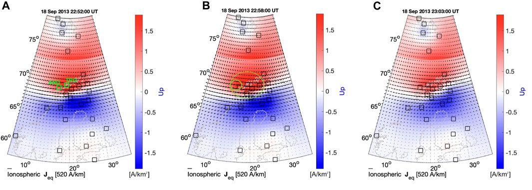
FIGURE 2. Direction of equivalent ionospheric currents (Jeq) shown as black arrows derived from IMAGE magnetometer stations (black squares) around the time of the auroral spiral. Colors depict the curl of equivalent currents, which is an estimate for field-aligned currents (FAC). (A) 22:52 UT, (B) 22:58 UT and (C) 23:03 UT. The dotted green ellipse marks the region of field of view from Tromsø with zenith angle 72°. The solid green ellipse shows an estimate for the size of the optical auroral spiral.
2.2 Cluster and THEMIS measurements
Measurements from three of the Cluster spacecraft (in the following called Cl1, Cl2 and Cl4) and the THEMIS-A (TH-A) satellite were obtained from Cluster Science Archive (Laakso et al., 2010) and NASA CDAweb, respectively. At the time of the spiral observation the Cluster and THEMIS-A spacecraft were positioned in the magnetotail (see Figure 3). The retrieved magnetic field measurements, plasma flow velocity and electron flux, temperature and density are displayed in Figure 4 for the time period of 22:40 UT to 23:10 UT.
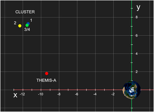
FIGURE 3. Position of the Cluster and THEMIS-A satellites at the time of the auroral spiral observation.
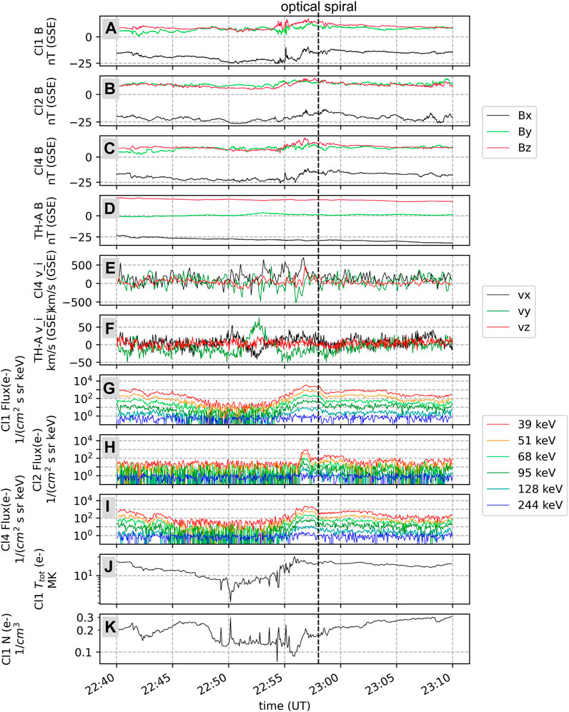
FIGURE 4. Data from Cl1, Cl2, Cl4 and TH-A on 18 September 2013 from 22:40 to 23:10 UT. (A–D) magnetic field measured by FGM instruments. (E, F) plasma flow velocities derived from data from CIS (Cluster) and ESA (TH-A) instruments. (G–I) electron flux for a range of energies measured by the Cluster RAPID instruments. (J, K) total electron temperature and density from the Cl1 PEACE instrument. The vertical dotted line shows the time of the spiral observation on the ground (22:58 UT). The data was retrieved from the Cluster Science Archive and NASA CDAweb.
The magnetic field (see Figures 4A–D) measured by FGM instruments shows dipolarization signatures for the Cluster spacecraft starting from ∼22:54 UT. The Cl1 data show a short peak in the BZ component around 22:55 UT, then a longer lasting increase with further peaks of the BZ component at 22:57 UT. These signatures known as dipolarizations are understood as the change of the magnetotail field from a stretched to a more dipolar configuration. Cl4 shows less distinct signatures than Cl1 around 22:55 UT, but also a peak of the BZ component at 22:57 UT. The satellite located farthest from Earth, Cl2, shows less variation than the other Cluster spacecraft in all magnetic field components, but also enhancements at 22:57 UT. In the TH-A magnetic field data no large perturbations are visible over the whole regarded time period. The Y component is near zero for the whole interval with a slight increase at ∼22:53 UT. The X and Z components constantly decrease from 22:40 UT to 23:10 UT.
The plasma flow velocities (see Figures 4E, F) were obtained from measurements by the Cl4 CIS-CODIF instrument and the TH-A ESA instrument. For the examined time interval, only the Cl4 CIS-CODIF instrument was operational. Enhanced quasi-periodical plasma flows can be discerned in its data from ∼22:50 to ∼22:58 UT. With a period of ∼2 min, the velocity in X direction (GSE) increases repeatedly to over ∼500 km s−1 before receding to ∼0 km s−1. The Y component shows the same development, with peak velocities of up to ∼500 km s−1 in negative Y direction (GSE). From about 2 min before the development of the optical auroral spiral in Tromsø, the deviations in X and negative Y direction (GSE) were most pronounced and the Z component showed enhanced flows of up to ∼500 km s−1. TH-A measured plasma flow that was slower than the Cl4 flow by one order of magnitude. Flow enhancements in the TH-A data starting at ∼22:49 UT can be seen in Figure 4F, which approximately concurs with the start of the high-speed flows visible in the Cluster data. The TH-A plasma velocity fluctuated between ∼40 km/s in positive and negative X directions (GSE). The Y component also fluctuated with peak velocities of ∼40 km s−1 and ∼70 km s−1 in dawn and dusk direction, respectively. These deviations in the TH-A flow velocity last only up to ∼22:56 UT.
The electron flux data from the Cluster RAPID instrument and the TH-A SST instrument is shown in Figures 4G–J. In the Cl2 data plots, strong signatures of dispersionless electron injections are discernible around 22:57 UT. Only the TH-A electron flux measurements with good data quality are displayed. The presented energy levels are not equal, but comparable to the Cluster energy channels. In the intervals where data with good quality was available, no variations in electron flux can be observed, while for the time of most interest no measurements are available.
In the interval between 22:49—22:56 UT the Cl1 electron total temperature and density (Figures 4J, K) measured by the PEACE instrument show quasi-periodical spikes in the electron density at the same time as sharp dips in the temperature. This dense and cold plasma alternates periodically with depleted and hot plasma, which is a typical signature of Kelvin-Helmholtz vortices (Hasegawa et al., 2009).
Overall, the Cluster data show deviations in all observed parameters up to 9 min precursory of the development of the visible auroral spiral in Tromsø.
3 Methods
3.1 Mapping
To correlate the spiral observations with their respective source regions in the magnetosphere, magnetic field line mapping was applied. Firstly, to determine the ionospheric footprints of the Cluster and TH-A satellites for the 18 September 2013 substorm, and, in particular, the time of the auroral spiral observation (22:58 UT). Secondly, a possible source region of the spiral was determined to evaluate if the structures observed by the spacecraft can have been correlated with the auroral spiral.
For these processes, the Python-based module IrbemPy, which is based on the IRBEM-lib library (Boscher et al., 2010) was used. It is part of the Python package SpacePy (Morley et al., 2010). As input options for the computation, the International Geomagnetic Reference Field (Erwan et al., 2015) was chosen as the internal magnetic field model and set to be updated on 18 September 2013. As the external magnetic field model, the Tsyganenko 1996 (T96) (Tsyganenko, 1995; Tsyganenko, 1996) magnetospheric model as stated below was selected. It was chosen above newer models, because it is also used in similar research (e.g., Keiling et al. (2009a)) and the T02 and T05 models primarily represent stormy or quiet conditions, while the here regarded event occurred during a substorm (Tsyganenko, 2002; Tsyganenko and Sitnov, 2005). For the mapping, the hourly values of the Kp, Dst and AL indices, as well as the solar wind density, velocity and dynamic pressure and the IMF BY and BZ components were obtained from the NASA/GSFC’s OMNI data set through the OMNI module (Morley et al., 2010).
3.1.1 Ionospheric footprints
The footprints of the magnetic field lines conjunct with the Cluster and TH-A spacecraft were derived using IrbemPy and position data retrieved from the Cluster Science Archive and NASA CDAweb. They are defined here as intercept points of these field lines and the ionosphere at an altitude of 100 km in the northern hemisphere. From 21:00 UT to 02:00 UT, the footprints lie in the area of the auroral oval in the dusk sector (see Figure 5). At 22:58 UT, the time of the auroral spiral observation, the footprints are located at longitudinal distances from Tromsø of
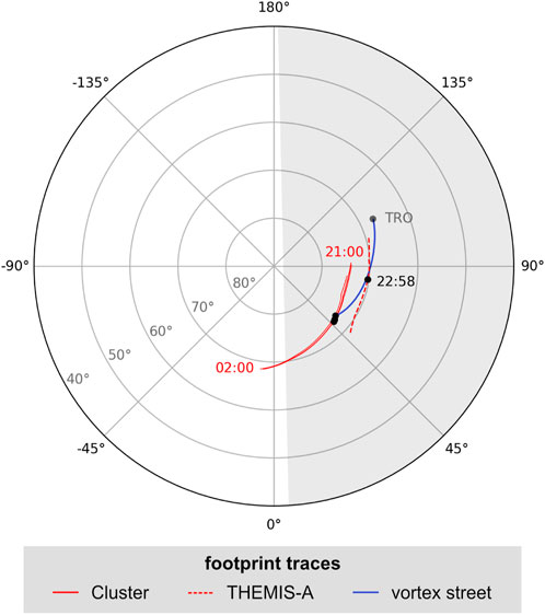
FIGURE 5. Ionospheric footprints of the Cl1, Cl2, Cl4 and TH-A spacecraft on 18/19 September 2013 plotted onto a geomagnetic grid with marked terminator for 22:58 UT. The red lines show the ionospheric footprints from 21:00 UT to 02:00 UT. For the time of the visible auroral spiral (22:58 UT) the footprints are designated with a black dot. Tromsø is marked with a gray dot. The blue line marks the propagation of the observed vortex street toward the spiral source region.
3.1.2 Spiral generator region
A possible magnetospheric generator region of the auroral spiral was derived with the constraint of it being conjunct with Tromsø by a magnetic field line. As explained below, the Cluster satellites observed Kelvin-Helmholtz vortices and it is suggested that after encountering the satellites these vortices possibly traveled to the generator region mentioned here, where they mapped down to the ionosphere to produce the optical spiral. Starting from the location of the Cl4 satellite at 22:58 UT, the coordinates were iteratively varied until their footprint was located in a radius of less than 50 km around Tromsø using the T96 model and IrbemPy. A potential source region of the spiral is thus located at around XGSE = −3.8 RE, YGSE = −1.7 RE and ZGSE = 2.4 RE. The absolute distance of this area to the Cluster satellites amounts to ∼12.1 RE.
3.2 Minimum variance analysis
To suitably display and analyze the spacecraft data in a local spacecraft coordinate system, Minimum Variance Analysis (MVA) as first proposed by Sonnerup and Cahill Jr (1967), was performed on the magnetic field and ion velocity data sets of Cl1, Cl2, Cl4 and TH-A. For TH-A the results of this method are not presented in the following, because the weak structures it detected were better displayed in the GSE coordinate system.
The method of MVA used here was derived from Sonnerup and Scheible (1998); Dunlop et al. (1995). In the time interval from 22:40 UT to 23:10 UT, the times of the maximum in the BZ (GSE) component of the Cluster magnetic field measurements were identified. For Cl1 the maximum was at 22:57:06 UT, for Cl2 at 22:57:37 UT and for Cl4 at 22:56:45 UT. A time period of 10 min symmetrically around 22:57:26 UT was selected for all Cluster satellites, this being the medium point in time between the Cl4 and Cl2 BZ maximum values. This interval was used for MVA calculations for each satellite to enable comparisons and showed reasonably good results for all three spacecraft.
The calculated eigenvalues and eigenvectors of the magnetic variance matrix (Dunlop et al. (1995); Sonnerup and Scheible, 1998) are listed in Table 1. The eigenvalues of the variance matrix describe the deviations of the field in the respective field directions, with the eigenvector n of the smallest eigenvalue (λ3) pointing in the expected direction of the boundary normal (Sonnerup and Scheible, 1998). The ratio λ2/λ3 is a measure for the quality of the direction estimates. Dunlop et al. (1995) give values of two to three for the λ2/λ3 ratio as a typical guideline. Here, the λ2/λ3 ratios were ∼2.0 for Cl1, ∼3.5 for Cl2 and ∼2.6 for Cl4 (see Table 1). As can be seen, the variance matrix is nearly degenerate for the three satellites, i.e., λ3 ≃ λ2. The boundary normal n is therefore not very well defined, although the eigenvector l is a good representation of a tangential direction to the boundary layer (Sonnerup and Scheible, 1998). According to Sonnerup and Scheible (1998), for near-degenerate cases, the eigenvectors m and n are prone to permute when modifying the time period for the calculation. As stated by Sonnerup and Scheible (1998) and Song and Russell (1999), this can be analyzed by executing the above method with different nested time intervals between 22:40 and 23:10 UT. All other time periods essentially showed similar λ2/λ3 ratios and highly changing directions of the eigenvectors m and n implying that the observed structure is 3-dimensional. The MVA in this case is not applicable.
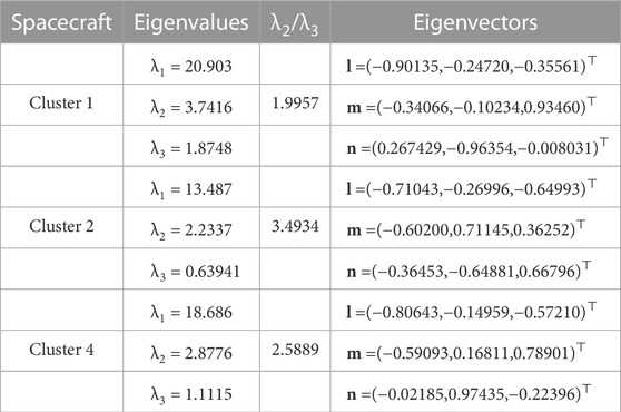
TABLE 1. Values from the Minimum Variance Analysis for an interval of 10 min around 22:57:26 UT performed on the Cluster magnetic field data.
For identification of the vortical structures in the magnetic field and ion flow velocity we can use an arbitrary orthogonal coordinate system. We have decided to use the one obtained above because it is orthogonal according to the dot product between the eigenvectors. The axes of the resulting LMN system are shown in Figure 6 with respect to the GSE coordinate system. The axes are defined so that the basis vectors l, m and n are parallel to the equivalent L, M and N axes. As can be seen, the direction of maximum variance l coincides approximately with the X (GSE) direction for all three Cluster satellites. However, the orientation of m and n varies for the satellites because the moving structure is 3D.
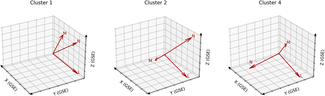
FIGURE 6. Axes of the LMN coordinate system (shown in red) with respect to the GSE coordinate system for the three used Cluster spacecraft.
The transformed magnetic field and ion flow velocity were projected to the L-M plane of the LMN coordinate system (see Figure 7). The TH-A data was accordingly projected to the X-Y (GSE) plane for the whole time period of 22:40 to 23:10 UT (see Figure 8). The Cluster magnetic field vector projections show rotational signatures in the time interval of 22:56 to 22:59 UT. Cl2, the most remote satellite, shows three major variations in sign of the BL component. Cl1 and Cl4, which were located closer together and nearer to Earth than Cl2, show one rotational signature coinciding with the first change of sign for the Cl2 BL component. For Cl1, which was closest to Earth, the signature is weaker than for Cl4. The vector projection of the plasma velocity does not show changes in sign for the vL component, but a change in the predominant vM direction in the time interval from 22:57 to 22:59 UT. The TH-A magnetic field data shows a change of sign of the BY component around 22:57 UT. Its plasma velocity also shows major variations of the vY component to positive and then negative values in the time period of 22:52 to 22:55 UT.
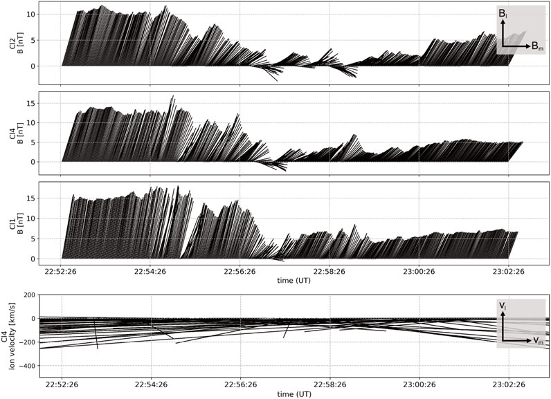
FIGURE 7. Magnetic field vectors of Cl2, Cl4 and Cl1 in this order and plasma velocity vectors from Cl4 projected onto the L-M plane of the LMN coordinate system versus time for a time interval containing the observation of the optical auroral spiral.
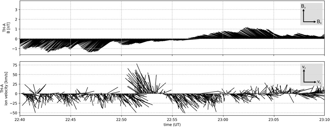
FIGURE 8. Magnetic field vectors and plasma velocity vectors from TH-A projected onto the X-Y plane (GSE) versus time for a time interval containing the observation of the optical auroral spiral.
4 Discussion
On 18 September 2013 at 22:58 UT, an auroral spiral was observed in Tromsø during the expansion phase of a substorm. Simultaneously, measurements in the magnetotail by three Cluster and the THEMIS-A spacecraft were obtained.
The three Cluster spacecraft measured strong variations in the magnetic field components, the plasma flow velocity and the electron flux approximately 1–2 min prior to the spiral development in Tromsø (see Figure 4). The plasma flow velocity from Cl4 over a time interval of 8 min showed quasi-periodic peaks in velocity up to ∼500 km s−1 in X and Y directions. These measurements correspond to the signatures of bursty bulk flows with intermittent flow bursts (Angelopoulos et al., 1992). As they commonly are (Paschmann et al., 2003), these bursty bulk flows were accompanied by dipolarization signatures seen in the BZ magnetic field components. The vector plots of the Cluster magnetic field projected onto the L-M plane of the local LMN coordinate system, which varies for each spacecraft, also show vortical signatures (see Figure 7). Cl2 encountered a magnetic field vortex street approximately oriented in the X-Y plane (GSE) with opposed rotating vortices on either side of its trajectory, as shown in Figure 9. Cl1 and Cl4 only measured a pair of opposed rotating vortices located roughly in the X-Z plane (GSE). Cl1 and Cl4 were positioned close together, so it is likely that they observed the same pair of magnetic field vortices.
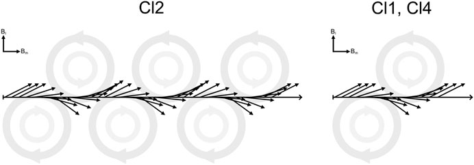
FIGURE 9. Illustration of the magnetic field vortices that can have caused the obtained vector measurements from Cl2, Cl1 and Cl4 shown in the L-M plane of the local spacecraft coordinate system LMN and along an idealized satellite trajectory.
If the frozen-in condition is valid, it is expected that the magnetic field vortices are connected to plasma flow vortices. The plasma flow velocity observed by Cl4 exhibited a change of direction at the occurrence of the magnetic field vortices, which suggests a vortical structure. Clear signatures of plasma vortices were not detected by the Cl4 spacecraft, likely because the CIS instrument used to measure the plasma velocity has a time resolution of ∼4 s. The magnetic field vortices however occurred at a temporal scale of ∼30 s.
These magnetic field vortices were probably associated with the bursty bulk flows that were also measured by Cl4. Bursty bulk flows are known to cause vortical structures in plasma flow in the X-Y (GSM) plane, when they encounter the dipolarized region of the inner magnetosphere (e.g., Panov et al., 2010; Birn et al., 2011). It was also observed by e.g., Volwerk et al. (2007) that Kelvin-Helmholtz instabilities appear together with bursty bulk flows. Hasegawa et al. (2004) detected plasma flow and magnetic field signatures caused by a Kelvin-Helmholtz instability at the magnetopause. Their magnetic field perturbations are different than shown in Figure 7, because the perturbations in our study are probably caused by pairs of oppositely rotating vortices, not by a single vortex street. TH-A was located closer to Earth and did not measure any vortical structures (see Figure 8). As seen in Figures 4J, K, Cl1 observed signatures in the electron temperature and density that are typical for Kelvin-Helmholtz instability, similar to Cluster observations described by Hasegawa et al. (2009). Therefore, the Cluster satellites likely observed a Kelvin-Helmholtz-like vortex street in the magnetic field induced locally by the measured bursty bulk flows. It has however to be taken into account that part of these results are based on the MVA, which produced results that were not ideally reliable.
Keiling et al. (2009b) observed short-lived equivalent ionospheric current vortices of 600–800 km size associated with the appearance of auroral spirals. In this study, such short-lived vortical Jeq structures could not be resolved. This can be due to the size of the auroral spiral (189 ± 45 km) and the comparative spatial resolution of the IMAGE magnetometer network. The stations in the vicinity of Tromsø have an average calculated distance of
To be able to correlate the ground observations and space measurements, the ionospheric footprints of the satellites were derived with the T96 external magnetic field model. They were located in the pre-midnight sector of the auroral oval (see Figure 5). The footprints lay at a distance from Tromsø of
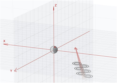
FIGURE 10. Schematic illustration of the vortex street oriented roughly in the X-Y (GSE) plane observed by Cl2 and its propagation towards the spiral source region (not to scale).
Following from the above calculation it can be possible that the magnetic field vortices, associated bursty bulk flows, KHI and dipolarizations detected by the spacecraft and described above were correlated with the spiral formation. What must be emphasized again, however, is the high uncertainty in the field line mapping during substorm conditions. This makes these interpretations mostly suggestions for a generation mechanism of the auroral spiral, based more on the temporal correlation of the vortices in the magnetotail and the optical spiral than on the exact spatial positions.
This suggestion proposes the spiral formation taking place already in the magnetosphere, not only in the ionosphere. Therefore, taking into account the available data, the spiral generation theory presented by Hallinan (1976) is not applicable to this event, since it states that the spiral only fully develops in the ionosphere.
According to a theory by Keiling et al. (2009b), plasma flow vortices in the magnetosphere are the initiator of a spiral, which then maps to ionospheric altitudes. These vortex structures can in turn be caused by either ballooning instabilities (e.g., Voronkov et al. (1997)) or bursty bulk flows (Keiling et al., 2009a; Panov et al., 2010). On encountering the dipolarized magnetic field in the inner magnetosphere, the high-speed plasma flows are decelerated (Panov et al., 2010; Birn et al., 2011). By their deflection around the dipolar magnetic field, vortices with opposed sense of rotation form on both sides of the flows (Panov et al., 2010).
5 Conclusion
The observations of dipolarizations and bursty bulk flows in this study coincide with the theory by Keiling et al. (2009b). In contrast to the detected structures of this event, Keiling et al. (2009b) also observed opposed rotating Jeq vortices that developed and decayed concomitant with auroral spirals. They associated these vortices with upward and downward field-aligned currents, which were driven in the magnetosphere by a pair of vortical plasma flows. According to Keiling et al. (2009b), the generation of the auroral spiral was likely initiated in the region of strong plasma flows between the plasma flow vortices in the magnetosphere. Here, such conclusions can not be drawn in the same way, because there were no equivalent ionospheric current vortices detected. The evidence of a vortex pair of Jeq in the ionosphere connected to plasma flow vortices in the magnetosphere was also not given. This can be due to the lack of mesoscale observations that can resolve these structures. However, with ∼500 A km−1 the westward electrojet current observed was stronger than an average substorm expansion current (Juusola et al., 2015), which may have helped establish an the instability for the spiral formation. Also, the magnetic field and possibly plasma vortices observed in the magnetotail caused by the eastward bursty bulk flows can have propagated toward the spiral source region and then mapped to the ionosphere as proposed similarly by Keiling et al. (2009b).
For future research on the interaction of magnetosphere and ionosphere in the generation of auroral spirals extended mesoscale observations in the ionosphere are needed. Also, for optical detection of auroral spiral events complementary to all sky cameras, citizen science projects like Aurorasaurus (MacDonald et al., 2015) are helpful.
Data availability statement
The datasets presented in this study can be found in online repositories. The names of the repository/repositories and accession number(s) can be found below: https://csa.esac.esa.int/csa-web/(Cluster Science Archive) https://cdaweb.gsfc.nasa.gov (NASA CDAweb) https://space.fmi.fi/image/www/index.php? (IMAGE magnetometers).
Author contributions
EK provided the idea for this study and took the original photograph of the auroral spiral. KM made the plots and wrote the manuscript. NP provided the plots for equivalent ionospheric currents. All authors contributed to the article and approved the submitted version.
Funding
The work of EK and KM is supported by German Research Foundation (DFG) under number KR 4375/2-1 within SPP “Dynamic Earth.” EK also acknowledges the support by Volkswagen foundation under the number AZ 97 742.
Acknowledgments
We thank the institutes who maintain the IMAGE Magnetometer Array: Tromsø Geophysical Observatory of UiT the Arctic University of Norway (Norway), Finnish Meteorological Institute (Finland), Institute of Geophysics Polish Academy of Sciences (Poland), GFZ German Research Centre for Geosciences (Germany), Geological Survey of Sweden (Sweden), Swedish Institute of Space Physics (Sweden), Sodankylä Geophysical Observatory of the University of Oulu (Finland), Polar Geophysical Institute (Russia), DTU Technical University of Denmark (Denmark), and Science Institute of the University of Iceland (Iceland). The provisioning of data from AAL, GOT, HAS, NRA, VXJ, FKP, ROE, BFE, BOR, HOV, SCO, KUL, and NAQ is supported by the ESA contracts number 4000128139/19/D/CT as well as 4000138064/22/D/KS. We acknowledge use of NASA/GSFC’s Space Physics Data Facility’s CDAWeb service, and OMNI data. We acknowledge the use of the IRBEM library (V.4.3), the latest version of which can be found at https://doi.org/10.5281/zenodo.6867552.
Conflict of interest
The authors declare that the research was conducted in the absence of any commercial or financial relationships that could be construed as a potential conflict of interest.
Publisher’s note
All claims expressed in this article are solely those of the authors and do not necessarily represent those of their affiliated organizations, or those of the publisher, the editors and the reviewers. Any product that may be evaluated in this article, or claim that may be made by its manufacturer, is not guaranteed or endorsed by the publisher.
References
Angelopoulos, V., Baumjohann, W., Kennel, C. F., Coroniti, F. V., Kivelson, M. G., Pellat, R., et al. (1992). Bursty bulk flows in the inner central plasma sheet. J. Geophys. Res. Space Phys. 97, 4027–4039. doi:10.1029/91JA02701
Birn, J., Nakamura, R., Panov, E. V., and Hesse, M. (2011). Bursty bulk flows and dipolarization in MHD simulations of magnetotail reconnection. J. Geophys. Res. Space Phys. 116. doi:10.1029/2010JA016083
Boscher, D., Bourdarie, S., O’Brien, P., and Guild, T. (2010). IRBEM library V4.3, 2004-2008. Toulouse France: ONERA-DESP.
Davis, T. N., and Hallinan, T. J. (1976). Auroral spirals, 1. Observations. J. Geophys. Res. 81, 3953–3958. doi:10.1029/JA081i022p03953
Dunlop, M., Woodward, T., and Farrugia, C. (1995). “Minimum variance analysis: Cluster themes,” in Proceedings of the cluster workshops. Editors K.-H. Glassmeier, U. Motschmann, and R. Schmidt (Braunschweig, Germany: ESA Special Publication), 33.
Erwan, T., Finlay, C., Beggan, C., Alken, P., Aubert, J., Barrois, O., et al. (2015). International geomagnetic reference field: the 12th generation. Earth, Planets Space 67, 79. doi:10.1186/s40623-015-0228-9
Gabrielse, C., Gkioulidou, M., Merkin, S., Malaspina, D., Turner, D., Chen, M., et al. (2023). Mesoscale phenomena and their contribution to the global response: a focus on the magnetotail transition region and magnetosphere-ionosphere coupling. Front. Astronomy Space Sci. 10, 1151339. doi:10.3389/fspas.2023.1151339
Hallinan, T. J. (1976). Auroral spirals, 2. Theory. J. Geophys. Res. 81, 3959–3965. doi:10.1029/JA081i022p03959
Hasegawa, H., Fujimoto, M., Phan, T.-D., Rème, H., Balogh, A., Dunlop, M., et al. (2004). Transport of solar wind into Earth’s magnetosphere through rolled-up Kelvin–Helmholtz vortices. Nature 430, 755–758. doi:10.1038/nature02799
Hasegawa, H., Retinò, A., Vaivads, A., Khotyaintsev, Y., André, M., Nakamura, T., et al. (2009). Kelvin-helmholtz waves at the earth’s magnetopause: multiscale development and associated reconnection. J. Geophys. Res. 114. doi:10.1029/2009JA014042
Juusola, L., Kauristie, K., van de Kamp, M., Tanskanen, E. I., Mursula, K., Asikainen, T., et al. (2015). Solar wind control of ionospheric equivalent currents and their time derivatives. J. Geophys. Res. Space Phys. 120, 4971–4992. doi:10.1002/2015JA021204
Juusola, L., Kauristie, K., Vanhamäki, H., Aikio, A., and van de Kamp, M. (2016). Comparison of auroral ionospheric and field-aligned currents derived from swarm and ground magnetic field measurements. J. Geophys. Res. Space Phys. 121, 9256–9283. doi:10.1002/2016JA022961
Keiling, A., Angelopoulos, V., Runov, A., Weygand, J., Apatenkov, S. V., Mende, S., et al. (2009a). Substorm current wedge driven by plasma flow vortices: THEMIS observations. J. Geophys. Res. Space Phys. 114. doi:10.1029/2009JA014114
Keiling, A., Angelopoulos, V., Weygand, J. M., Amm, O., Spanswick, E., Donovan, E., et al. (2009b). THEMIS ground-space observations during the development of auroral spirals. Ann. Geophys. 27, 4317–4332. doi:10.5194/angeo-27-4317-2009
Laakso, H., Perry, C., McCaffrey, S., Herment, D., Allen, A., Harvey, C., et al. (2010). “Cluster active archive: overview,” in The cluster active archive. Editors H. Laakso, M. Taylor, and C. Escoubet (Dordrecht: Springer), 3–37.
MacDonald, E. A., Case, N. A., Clayton, J. H., Hall, M. K., Heavner, M., Lalone, N., et al. (2015). Aurorasaurus: A citizen science platform for viewing and reporting the aurora. Space Weather. 13, 548–559. doi:10.1002/2015SW001214
Met Office (2010-2015). Cartopy: a cartographic python library with a matplotlib interface. Exeter, Devon. Available at: https://scitools.org.uk/cartopy
Morley, S., Welling, D., Koller, J., Larsen, B., Henderson, M., and Niehof, J. (2010). “Spacepy - a python-based library of tools for the space sciences,” in Proceedings of the 9th Python in science conference. Editors S. van der Walt, and J. Millman Austin, TX, 67–72.
Panov, E. V., Nakamura, R., Baumjohann, W., Angelopoulos, V., Petrukovich, A. A., Retinò, A., et al. (2010). Multiple overshoot and rebound of a bursty bulk flow. Geophys. Res. Lett. 37. doi:10.1029/2009GL041971
Partamies, N., Freeman, M. P., and Kauristie, K. (2001a). On the winding of auroral spirals: interhemispheric observations and hallinan’s theory revisited. J. Geophys. Res. Space Phys. 106, 28913–28924. doi:10.1029/2001JA900093
Partamies, N., Kauristie, K., Pulkkinen, T. I., and Brittnacher, M. (2001b). Statistical study of auroral spirals. J. Geophys. Res. Space Phys. 106, 15415–15428. doi:10.1029/2000JA900172
Paschmann, G., Haaland, S., and Treumann, R. (2003). Auroral plasma Physics. Dordrecht: Springer Science+Business Media. doi:10.1007/978-94-007-1086-3
Song, P., and Russell, C. (1999). Time series data analyses in space Physics. Space Sci. Res. 87, 387–463. doi:10.1023/A:1005035800454
Sonnerup, B. U. O., and Cahill, L. J. (1967). Magnetopause structure and attitude from Explorer 12 observations. J. Geophys. Res. 72, 171–183. doi:10.1029/JZ072i001p00171
Sonnerup, B. U. Ö., and Scheible, M. (1998). Minimum and maximum variance analysis. ISSI Sci. Rep. Ser. 1, 185–220. Available at: https://api.semanticscholar.org/CorpusID:118577335
Tsyganenko, N. A. (2002). A model of the near magnetosphere with a dawn-dusk asymmetry 2. Parameterization and fitting to observations. J. Geophys. Res. Space Phys. 107, SMP 10-11–SMP 10-17. doi:10.1029/2001JA000220
Tsyganenko, N. A. (1996). “Effects of the solar wind conditions in the global magnetospheric configurations as deduced from data-based field models,” in International conference on substorms. Editors E. J. Rolfe, and B. Kaldeich (ESA Special Publication), 181.
Tsyganenko, N. A. (2001). “Empirical magnetic field models for the space weather program,” in Space weather. Editors H. S. P. Song, and G. Siscoe (Washington, D. C: American Geophysical Union), 273–280.
Tsyganenko, N. A. (1995). Modeling the Earth’s magnetospheric magnetic field confined within a realistic magnetopause. J. Geophys. Res. Space Phys. 100, 5599–5612. doi:10.1029/94JA03193
Tsyganenko, N. A., and Sitnov, M. I. (2005). Modeling the dynamics of the inner magnetosphere during strong geomagnetic storms. J. Geophys. Res. Space Phys. 110, A03208. doi:10.1029/2004JA010798
Untiedt, J., and Baumjohann, W. (1993). Studies of polar current systems using the IMS Scandinavian magnetometer array. Space Sci. Rev. 63, 245–390. doi:10.1007/BF00750770
Volwerk, M., Glassmeier, K.-H., Nakamura, R., Takada, T., Baumjohann, W., Klecker, B., et al. (2007). Flow burst-induced Kelvin-Helmholtz waves in the terrestrial magnetotail. Geophys. Res. Lett. 34, L10102. doi:10.1029/2007GL029459
Voronkov, I., Rankin, R., Frycz, P., Tikhonchuk, V. T., and Samson, J. C. (1997). Coupling of shear flow and pressure gradient instabilities. J. Geophys. Res. Space Phys. 102, 9639–9650. doi:10.1029/97JA00386
Keywords: auroral spiral, bursty bulk flows, Kelvin-Helmholtz instability, substorm, aurora
Citation: Maetschke KN, Kronberg EA, Partamies N and Grigorenko EE (2023) A possible mechanism for the formation of an eastward moving auroral spiral. Front. Astron. Space Sci. 10:1240081. doi: 10.3389/fspas.2023.1240081
Received: 14 June 2023; Accepted: 26 September 2023;
Published: 13 October 2023.
Edited by:
Dimitry Pokhotelov, German Aerospace Center (DLR), GermanyReviewed by:
Joachim Vogt, Jacobs University Bremen, GermanyIldiko Horvath, The University of Queensland, Australia
Copyright © 2023 Maetschke, Kronberg, Partamies and Grigorenko. This is an open-access article distributed under the terms of the Creative Commons Attribution License (CC BY). The use, distribution or reproduction in other forums is permitted, provided the original author(s) and the copyright owner(s) are credited and that the original publication in this journal is cited, in accordance with accepted academic practice. No use, distribution or reproduction is permitted which does not comply with these terms.
*Correspondence: Elena A. Kronberg, a3JvbmJlcmdAZ2VvcGh5c2lrLnVuaS1tdWVuY2hlbi5kZQ==