Using the Perseverance MEDA-RDS to identify and track dust devils and dust-lifting gust fronts

In the framework of the Europlanet 2024 Research Infrastructure Transnational Access programme, a terrestrial field campaign was conducted from 29 September to 6 October 2021 in Makgadikgadi Salt Pans (Botswana). The main goal of the campaign was to study in situ the impact of the dust devils (DDs) on the observations made by the radiometer Radiation and Dust Sensor (RDS), which is part of the Mars Environmental Dynamics Analyzer instrument, on board NASA’s Mars 2020 Perseverance rover. Several DDs and dust lifting events caused by non-vortex wind gusts were detected using the RDS, and the different impacts of these events were analyzed in the observations. DD diameter, advection velocity, and trajectory were derived from the RDS observations, and then, panoramic videos of such events were used to validate these results. The instrument signal variations produced by dust lifting (by vortices or wind gusts) in Makgadikgadi Pans are similar to those observed on Mars with the RDS, showing the potential of this location as a Martian DD analog.

1 Introduction

Dust devils (DDs) are dry, dusty convective vortices that play a major role in the Mars dust cycle Newman et al., 2002; Basu et al., 2004). Their horizontal wind speeds are intense enough to transport the dust available on the surface into the atmosphere, and there, the lifted dust particles can directly affect the energy balance of the planet by absorbing and scattering the solar radiation (Changela et al., 2021). Furthermore, dust particles in the swirling DDs may become electrically charged via triboelectric effects (Farrell et al., 2004) and lead to the aggregation of the dust grains. Although the exact DD contribution to the global atmospheric dust budget is still under discussion, some modeling works have suggested values of approximately 50% of the total budget (Kahre et al., 2006). However, the need for model validation against DD observations (e.g., DD frequency of formation and temporal variability) leads to uncertainties in the relative DD contributions in comparison to other dust-lifting mechanisms. For example, recent observations have demonstrated that outside the dust storm season, dust lifting (DL) by convectively driven wind gusts could raise amounts of dust similar to those due to DDs (Newman et al., 2022). Another important aspect of the DDs is their impact on the distribution of dust particles throughout the surface (concentration and size distribution), which affects the planet’s thermal inertia and surface albedo (Martínez et al., 2023; Vicente-Retortillo et al., 2023). Thermal inertia determines surface and shallow subsurface temperatures, and thus, variations in this geophysical property of the terrain might occasionally favor the formation of brine through deliquescence (Pál and Kereszturi, 2020).

The amount of dust transported from the surface into the atmosphere by a DD mainly depends on the dust flux (dust raised per unit area per time) and the DD lifetime (t_DD) and diameter (d_DD). By assuming the same dust flux for all the DDs and the relation between t_DD and t_DD given in the work of Lorenz (2013)(${\mathrm{t}}_{DD}\sim 0.66d_{DD}^{0.66}$), Toledo et al. (2023) used the product ${\rho }_{DD}\times {\bar{r}}_{DD}^{2.66}$, where ρ_DD and ${\bar{r}}_{DD}$ represent the DD frequency of formation and average radius, respectively, as a metric to compare two locations in terms of the amount of dust raised by DDs. Estimations of ρ_DD and ${\bar{r}}_{DD}$ at different locations and time periods (Ferri et al., 2003; Greeley et al., 2006; Fenton and Lorenz, 2015; Reiss et al., 2016; Perrin et al., 2020) show that these parameters (and so the amount of dust lifted by the DDs) are highly variable in time and from place-to-place. Thus, continuous DD observations (encompassing the diurnal cycle) at different locations are critical to establishing quantitative constraints on the DD contribution to the Martian dust budget.

Martian DDs have been observed and characterized (e.g., DD height and diameter or frequency of formation) from the following: 1) orbital images (Thomas and Gierasch, 1985; Fisher et al., 2005); 2) images obtained from surface platforms and rovers (Metzger et al., 1999; Greeley et al., 2006); 3) DD tracks visible on the surface (Verba et al., 2010; Hargitai and Kereszturi, 2015; Reiss et al., 2016; Perrin et al., 2020); 4) in situ observations of pressure, radiation, temperature, and wind (Ordóñez-Etxeberria et al., 2020; Kahanpää and Viúdez-Moreiras, 2021); and 5) currents registered by solar arrays (Lorenz et al., 2021). More recently, different works have analyzed data of irradiance, pressure, temperature, and wind collected from the Mars Environmental Dynamics Analyzer (MEDA) station (Rodriguez-Manfredi et al., 2021; Rodriguez-Manfredi et al., 2023) on board the Mars 2020 Perseverance rover (which landed on Mars on 18 February 2021 and has been operational since then) to study the properties of DDs, vortices, and events of DL produced by non-vortex wind gusts in the Jezero crater (Hueso et al., 2022; Jackson, 2022; Newman et al., 2022; Toledo et al., 2023). A main advantage of MEDA observations is the sampling frequency (1 Hz) and the temporal coverage: blocks of 1 h selected along the day based on a cadence that alternates between even and odd hours. Although the number of blocks sometimes changes depending on data volume and power availability, MEDA often covers around 12 h per day, which allows studying the diurnal cycle of the DDs and its seasonal variability.

One of the MEDA sensors is the Radiation and Dust Sensor (RDS) (Apestigue et al., 2022), which measures solar radiation at different wavelengths and incident geometries. As demonstrated by Apestigue et al. (2021) and Toledo et al. (2023), the RDS measurements are sensitive to the presence of DDs, and for some particular dust events, some information on the DD properties can be derived. In order to test the capabilities of the RDS to characterize DDs, a terrestrial field campaign was conducted from 29 September to 6 October 2021 in the Makgadikgadi Salt Pans (Botswana), an arid region where the formation of DDs is frequent during the dry season. Field campaigns in Martian analogs offer a chance for assessing and verifying the reliability of certain measurements for the characterization of DDs. In this regard, by acquiring elemental data of the DDs by reference instrumentation (e.g., cameras), it is possible to validate the RDS (or other instruments of interest) retrievals to an extent that is not possible on Mars (because of the limited number of instruments and observations). For the field measurements, we used the RDS terrestrial spare unit and several instruments to validate the DD retrievals. In this paper, we present the results obtained during the campaign and compare the RDS measurements with the data on Mars (acquired by MEDA on board Perseverance). The different DD products obtained from the RDS measurements were validated against images captured by two commercial cameras that operated continuously. This manuscript is organized as follows: in Section 2, we describe the different instruments involved in the field campaign and the field deployment; in Section 3, we present an overview of the data, characterize the impact of DD and DL caused by non-vortex wind gusts in the RDS signals, compare the DD observations with those made on Mars, and study the impact of the instrument sampling frequency on the detection and characterization of DDs; and in Section 4, we outline the main conclusions derived from this work.

2 Materials and methods

2.1 Instrumentation

The main instrument used in this campaign was the spare unit of the radiometer RDS (Apestigue et al., 2022) (see Figure 1A). The RDS is a part of the instrument Mars Environmental Dynamics Analyzer (Rodriguez-Manfredi et al., 2021; Rodriguez-Manfredi et al., 2023) on board NASA’s Mars 2020 Perseverance rover, which has been operational on the Martian surface for more than 2 terrestrial years. The RDS has two sets of photodetectors and a camera pointing at the zenith (not included in the spare unit). The first set of photodetectors, referred to as the Top channels, corresponds to eight detectors pointing at the zenith that cover the light spectrum from the ultraviolet to the near infrared (Top-1 to Top-8: 255 ± 5, 259 ± 5, 250–400, 450 ± 40, 650 ± 25, 750 ± 5, 190–1,100, and 950 ± 50 nm). Most of the Top detectors use interferential filters and mechanical masks to constrain their field of view (FOV) to ± 15° zenith angle, while the Top-7 channel covers the full sky. The second set of photodetectors are eight lateral channels, referred to as Lat channels, which are pointed sideways at 20° (except Lat-8, which is 35°) above the platform and are all in the wavelength range of 750 ± 5 nm. The Lat-1 channel is blinded to study the degradation of photodetector performance. The FOV of all the Lat sensors is ± 5°.

FIGURE 1

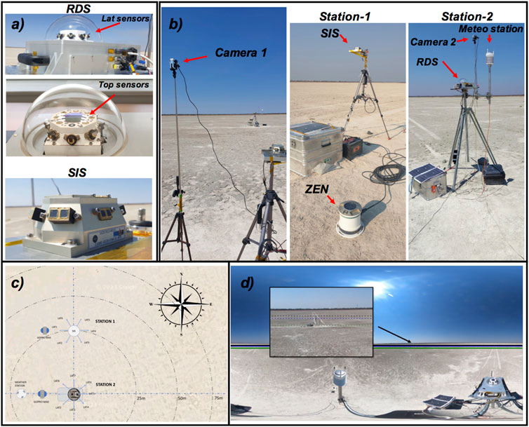
FIGURE 1. (A) Images of the RDS and SIS showing the disposition of the different sensors. SIS Top sensors correspond to four zenith-pointed detectors, which cover the following spectral bands: 255 ± 5 nm, 269 ± 5 nm, 250–400 nm, and 750 ± 5 nm. For the first two sensors, the FOV is constrained to ± 15° zenith angle, while for the other two, it is constrained to ± 40°. The second set corresponds to twelve Lat channels, grouped in pairs at two different spectral bands (250–400 and 750 ± 5 nm), pointing sideways at six different azimuth angles and 20° above the platform. The FOV of all the Lat sensors is constrained to ±5°. (B) Pictures of the field deployment. The instruments were placed at two different stations separated by approximately 25 m. The SIS and ZEN radiometers were installed in station-1, while the RDS and Vaisala weather station were in station 2. Both stations were equipped with a GoPro camera that was installed on tripods (as were the RDS, SIS, and Vaisala weather station). (C) Diagram showing how the instruments were deployed and oriented along the field. (D) Image taken by the GoPro camera at station 2. The green, blue, and black lines indicate the 25, 50, and 75 m radius concentric circles that were made on the ground.

In addition to the RDS, the following instruments are also used in the field campaign: i) the radiometer Solar Irradiance Sensor (SIS) (Arruego et al., 2016), which was selected to be part of the ExoMars 2022 Meteo package (not included anymore in the ExoMars mission). Similar to the RDS, the SIS has two sets of photodetectors (Top and Lat channels) with different spectral bands and FOVs (see Figure 1 for a full description); ii) a Vaisala weather station (model WXT-530) to perform measurements of pressure, wind speed and direction, temperature, and relative humidity; iii) 2 GoPro Max commercial cameras to record panoramic videos and identify the different dust events captured by the RDS and SIS; and iv) a ZEN radiometer (Almansa et al., 2017) to provide information about the aerosol opacity conditions. As on the Mars 2020 mission, the sampling frequency of the RDS was set at 1 Hz.

2.2 Dust-lifting detection with the RDS

Like for the clouds, the presence of DDs or DL caused by wind gusts produces changes in the sky brightness as a result of the interactions between sunlight and the lifted dust particles. If a DD or DL crosses the FOV of one or more of the of the RDS sensors, then these variations can be captured by the instrument as signal temporal variations. Their signature on the irradiance observations can be positive or negative (as observed in similar terrestrial analog observations with solar flux sensors (Lorenz and Jackson., 2015), depending on the DD dimensions (diameter and height) and opacity (dust load), as well as on the following observation properties: spectral bands, distance DD-RDS, and the DD and Sun angular positions (Toledo et al., 2023). As detailed in the following sections, the intensity of the detections, defined as the signal variations with respect to the background measurements, also depends on all these factors.

2.3 Makgadikgadi Pans and field deployment

The instruments were deployed in a small pan near the town of Mopipi (around latitude 21.22 ° S and longitude 24.86 ° E), in the central district of Botswana. This pan is part of the larger systems of ephemeral salt lakes called Makgadikgadi Pans that developed due to the gradual shrinking of a giant lake called Palaeo-Makgadikgadi that occupied the central Kalahari since the Upper Pleistocene (Franchi et al., 2022). The giant lake developed within the Makgadikgadi–Okavango–Zambezi Basin as part of the south-western branch of the East African Rift System, and its evolution is controlled by NE–SW-trending normal faults (Schmidt et al., 2023a). This is now one of the largest salt pan complexes on the planet and receives seasonal surface water from local rainfall, groundwater upwelling, and ephemeral rivers flowing from the east and northeast and, seasonally, from the Boteti River that terminates less than 10 km southwest of the study area. The region is characterized by ca. 300 mm/year of rain, mostly limited to the summer rainy season, between November and March, which is followed by a long dry winter (Franchi et al., 2022). During the winter dry season, the dominant processes are wind erosion and calcretization under playa-like conditions. It is for the overlaps of groundwater upwelling, evaporite processes, and wind erosion that the Makgadikgadi Pans have been identified as potential analogs of Mars playa deposits (Franchi et al., 2020; Schmidt et al., 2023b).

Measurements were conducted in September-October 2021, at the end of the dry season and before the seasonal winter rains. For each day of the campaign, the instruments were deployed in the morning and packed up at the end of the day. They were installed at ∼1.5 (station 1) and 2 (station 2) m height (except the ZEN radiometer that operated over the surface) on two different tripods (referred to as stations 1 and 2 in the right panels of Figure 1), separated by approximately 25 m (see Figure 1C). The objective of having the instruments at two different locations was to capture the dust events with different observing geometries. For the power supply, we utilized solar panels (as the campaign was conducted during daylight hours of maximum solar irradiance) and car batteries. The RDS was configured in an I-Box, a portable and embedded system designed in the INTA (Serrano et al., 2022), to prevent dust deposition over the sensors. All the instruments were controlled from a third station (station 3) located approximately 30 m away from stations 1 and 2. To estimate the distance of the DDs passing near the stations, several concentric circles with radii of 25, 50, 75, 100, 125, and 150 m were made on the ground. However, it was difficult to identify the concentric circles with radii greater than 75 m in the images (see Figure 1D). Thus, it was not possible to determine a distance reference for the events traveling at distances greater than 75 m. Operations on the first 2 days of the campaign were partially interrupted because of issues with the power supply and the system.

3 Results

3.1 Data overview

During the campaign, a total of eighteen DDs and events of DL caused by non-vortex wind gusts were detected by both the RDS and the cameras. Figure 2 shows an example of DD detection carried out by the RDS on September 30 (the second day of the campaign). The event was registered by Lat-2 and Lat-8 sensors (likely by Lat-3 too) and Top channels. It should be noted that Top-1 and Top-2 data are not displayed in Figure 2 because sunlight at these channel spectral bands is negligible at the surface (because of O₃ absorption). Here, it is observed that the signal variations produced by the DD are different in the Lat and Top channels: in the Lat channels, the encounter with the DD results in a sequence of detections, while in the Top channels, the maximum (or minimum for Top-3 and Top-4) occurs at the same time. Figures 3A,B illustrate a diagram of the intersection between a DD trajectory and the different sensors’ FOV. The Lat sensors’ FOVs are oriented at different azimuth angles, and thus, the intersection between the DD and the different sensors cannot occur at the same time (unless the DD is very close and covers all the instrument sensors). For Top channels, however, all the sensors have the same FOV (except Top-7, which is total sky), and thus, the detections must be at the same time. As we will see in Section 3.2, this different geometry of detections allows us to estimate DD properties such as d_DD or the trajectory. Interestingly, we observed from Figure 2 that the net impact of the DD depends on the spectral band: in Top-8, -6, and -5 channels, the DD increased the irradiance with respect to the background levels, while in Top-4 and -3 wavelength ranges, the DD impact was the opposite. The possible reasons for this result and the comparison with the Martian cases are discussed in Section 3.4.

FIGURE 2

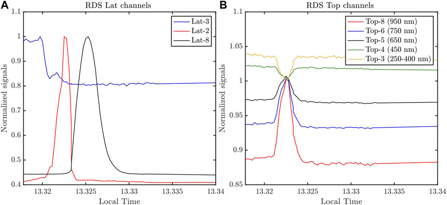
FIGURE 2. An example of a DD detected by the RDS Lat (A) and Top (B) sensors on the second day of the campaign (signals normalized by their respective maxima). For Lat-2 and -8 sensors, the DD produced increases of more than 50% (with respect to the background signals). The signal variation observed in Top sensors occurs when the DD is at its closest approach to the RDS, and the net impact (increase or decrease in irradiance) depends on the spectral band of the sensors.

FIGURE 3

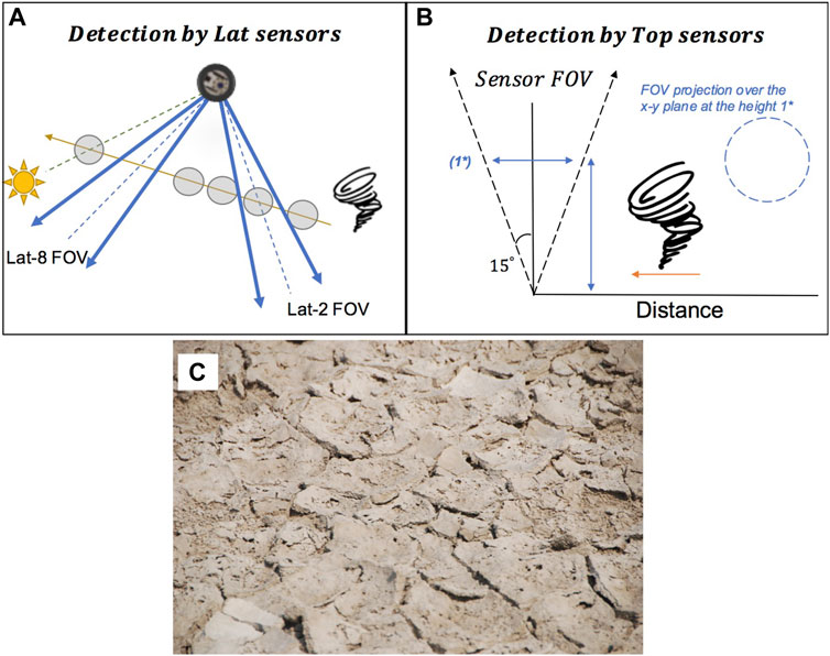
FIGURE 3. (A, B) Diagram showing the RDS Lat-2 and -8 (A) and Top (B) sensor orientations, along with the possible trajectory of the DD shown in Figure 2. For Top sensors, the height of the DD determines the maximum distance at which the DD can be detected (or the maximum distance at which the DD intersects the sensor FOV). (C) Field photo after the rainy day. Once the first layers of the ground dried out, desiccation cracks formed on the surface and little dust was available. After that, the DDs were less frequent and had a lower dust load.

Detections similar to those shown in Figure 2 were carried out by the RDS during the different days of the campaign. The DD frequency of formation, DD size, and dust load varied from day to day depending on the amount of dust available on the surface and the wind conditions. On our third day in the Pans (1 October 2021), the campaign had to be canceled due to rainy conditions. Despite lasting only a few hours, the rain left the ground slightly moist at some locations for the following days (especially the day after), and once dried, the mud was rather hard, and there was little dust (see Figure 3C). For this reason, the DDs (or DL caused by non-vortex wind gusts) after the rainy day were less dusty than those observed during the first 2 days.

Wind speed conditions influenced the formation of DDs or DL. Figure 4 shows the measurements of wind speed and direction made by the Vaisala station for the 6 days of the campaign (not 7 days because on 1 October 2021, the instrument deployment had to be canceled). The same temporal periods were covered by RDS observations. On the first day of the campaign, the wind speed was 3.7 ± 1.3 m s⁻¹ on average but with frequent wind gusts of 6 m s⁻¹ or above. DDs were very frequent during this day, but because of power supply issues, not all the events were registered by the instruments. For the second day, winds were stronger (7.5 ± 1.6 m s⁻¹ on average) with gusts of up to 14.5 m s⁻¹. During this day, events of DL caused by wind gusts were more frequent than DDs, and in some cases, we observed DDs that were suppressed by the winds (DDs sheared out by the strong winds). Yet, some DDs were formed and detected by the instruments (an example is the case shown in Figure 2, for which the background wind was between 6 and 11 m s⁻¹ around the detection).

FIGURE 4

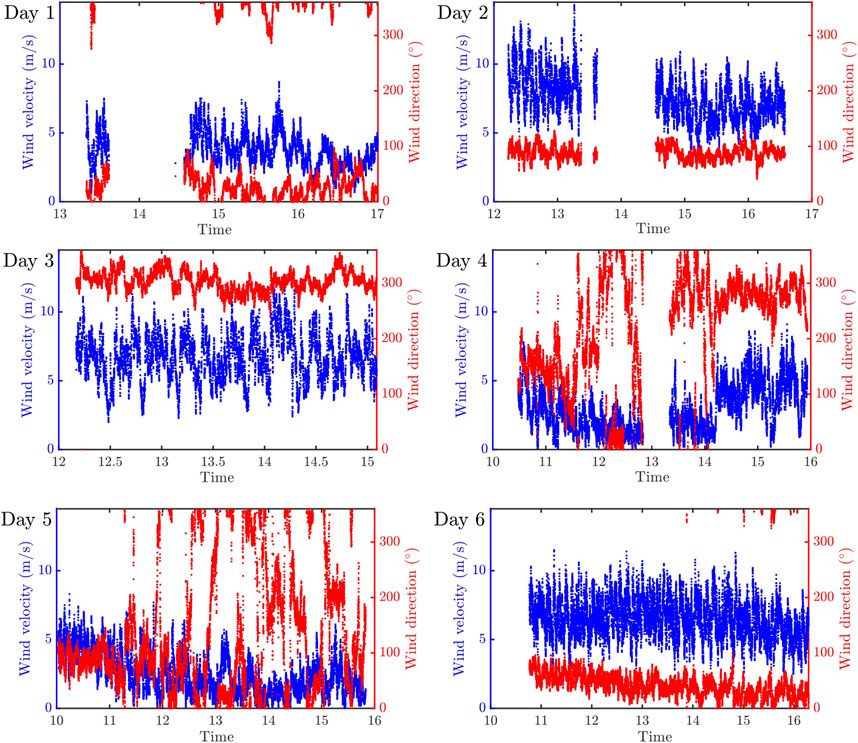
FIGURE 4. Diurnal variation in wind speed (blue axis on the left) and direction with respect to north (red axis on the right) measured by the Vaisala weather station during the 6 days of the campaign. The gaps in the measurements are due to issues with the power supply and the system.

For the rest of the days, average winds were 6.7 ± 1.7, 2.9 ± 1.7, 2.46 ± 1.4, and 6.5 ± 1.4 m s⁻¹. The DD frequency during these days was lower than that given for the first 2 days of the campaign. This could be due to a decrease in the number of vortices capable of lifting dust (because of the wind conditions), a decrease in the amount of dust available on the surface (for the previously discussed reasons), or a combination of these two factors. Previous works have studied the impact of the background wind speed on the DD frequency of formation. For instance, Oke et al. (2007) observed a total of 557 DDs at a field site in Australia and found that DD formation was restricted to background wind velocities between 1.5 and 7.7 m s⁻¹ with peak activity at ∼ 3 m s⁻¹. This is consistent with the measured wind conditions and the number of DDs observed during the campaign. On the first day, the wind speed at around 13 was 3.93 ± 1.43 m s⁻¹ on average, which is close to the peak in activity reported by Oke et al. (2007). On the contrary, for the second day, the average wind speed around the same time was close to the upper limit reported in the same work, which explains the different number of DDs observed during these 2 days. For the rest of the days (after the rainy conditions), the average wind speeds between 12 and 14 local time (that is, the time of the day when most of the DDs were detected) were 6.55 ± 1.65, 1.73 ± 0.90, 2.01 ± 1.15, and 6.81 ± 1.36 m s⁻¹, which are, except for day 5 of the campaign, well below or above the 3 m s⁻¹ peak reported by Oke et al. (2007). Thus, these results indicate that both factors (the wind conditions and the dust available on the surface) could have influenced the variability of the DD frequency of formation along the campaign.

Finally, we tried to study the population of vortices during the campaign using the Vaisala pressure observations. As shown in previous works (Sinclair, 1973), vortices can be detected by searching for the local drop in pressure expected with the vortex passage. Unfortunately, the pressure observations made by the Vaisala station did not have enough precision and sampling frequency to detect vortex passages (see the work of Lorenz. (2012) for more information about the precision and cadence required for detecting vortices or DDs with pressure loggers). Therefore, these observations were not used in this work. Figure 5 presents some images of DDs and DL caused by wind gusts observed during the campaign. The DDs shown in Figures 5A,B correspond to the first 2 days of the campaign, and the DD in Figure 5C (indicated with the black arrow) was observed 3 days after the rainy day. In general, and as shown in the figure, the dust load of the DDs was smaller after the rain.

FIGURE 5

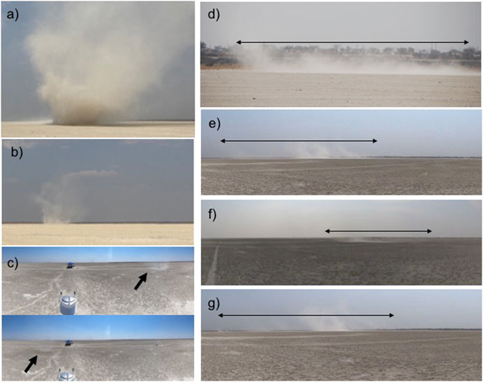
FIGURE 5. Examples of DDs (A–C) and wind gusts (D–G) observed during the field campaign. The DDs observed for the first 2 days of the campaign (A, B) were much dustier than those formed after the rainy day (C). In general, dust lifting caused by wind gusts has a larger horizontal extension (indicated with black arrows) than vertical extension (in contrast to the DDs, where d_DD < DD height).

3.2 Dust devil characterization with the RDS

The signal variations produced by DDs are specific and different from those produced by other factors (e.g., clouds). Figure 6A shows different signatures in RDS signals (Lat sensors) produced by the presence of DDs, clouds, and DL caused by wind gusts. Here, the duration of the increase produced by clouds (approximately 3–4 min) is much longer than that due to DDs (approximately 20 s). This is explained by the larger distance between the instrument and the cloud than between the instrument and the DD, making the sensor FOV projection larger too. For Lat sensors, the ratio between the time duration of a DD detection (T_DD) and a cloud detection (T_cloud) can be approximated as follows:

$\frac{T_{DD}}{T_{\mathit{cloud}}}\sim \frac{d_{\mathit{RDS-DD}}}{h_{\mathit{cloud}}}\cdot \frac{v_{\mathit{cloud}}}{v_{DD}}\cdot \mathit{tan}\left(20°\right),(1)$

where v_DD and v_cloud are the velocities of the DD and the cloud, respectively, d_RDS−DD is the distance between the RDS and the DD, and h_cloud is the altitude of the cloud. Here, we assumed that both the DD and the cloud cross the sensor FOV through the center and that their dimensions are negligible with respect to the FOV projections at the cloud and DD distances. For example, for a ratio v_cloud/v_DD = 5 and d_RDS−DD and h_cloud values of 400 m and 4,500 m, the time duration of a cloud detection is about five times longer than that of a DD. Although this ratio can change depending on the cloud and DD dimensions (and other parameters), signal variations longer than ∼1 min are, in general, not produced by the presence of DDs and can be discarded in the analysis.

FIGURE 6

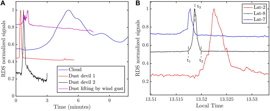
FIGURE 6. (A) Time duration of RDS Lat signal variations produced by two DDs, a DL caused by wind gusts and a cloud. The cloud detections generally last longer, and the signal variations are smoother than those due to a DD or a wind gust. (B) Sequence of RDS Lat detections produced by a DD encountered near the instrument on day 5 of the campaign.

In the case of DL caused by wind gusts, it is observed that the timescale of the detection is very similar to that of the DDs. However, as detailed in the following section, in general, the DDs are registered in the RDS observations as sequences of Lat detections (for the same event), while for the wind gust events, the signal variations are simultaneous (in case the DL is large enough to cover the FOV of more than one Lat sensor). Figure 6B shows an example of a DD detection carried out by the RDS on day 5 of the campaign. As in Figure 2, the different signals were normalized to their respective maxima. The DD was detected by three Lat channels (the sequence of detections does not include Lat-1 because this channel is blinded) and the Top sensors (not displayed in the figure). The fact that the Top sensors also detected the DD indicates that it passed in close proximity to the RDS. From the sequence of Lat detections and the orientation of the instrument, we infer that the DD had a trajectory coming from the northeast.

As demonstrated in the work of Apestigue et al. (2021) and Toledo et al. (2023), information on the DD velocity, trajectory (θ_DD, angle clockwise with respect to the north), and diameter can be derived from a sequence of RDS detections by fitting the measured times to a straight DD trajectory (referred to as DD trajectory analysis thereafter). Although the DD trajectories can be affected by terrain obstacles or other factors, in general, the DDs migrate with the background wind in somewhat straight lines (Balme et al., 2012; Lorenz, 2016). In addition, in our simulations, we assume DD is a dust column with no slope. For the Lat sensors, with a narrow FOV and pointing sideward at 20° above the platform, the slope is not expected to cause changes in the duration of each detection (which is the main parameter to retrieve the DD properties). For the Top detections, a DD tilted by 5° could have detection durations up to 10% longer than when the DD is not tilted, thus affecting the DD retrievals. However, for the estimation of the DD velocity, trajectory, and diameter, the Top detections are not used. For each Lat detection, three times are defined: the time when the detection starts (t₁), finishes (t₂), and reaches the signal maximum (t₃). These times are the moments when 1) the DD enters the sensor FOV; 2) the DD leaves the sensor FOV; and 3) the DD is at the center of the sensor FOV, where the light transmission is at its maximum. Thus, in the example shown in Figure 6B, we have a total of nine different times to fit. Once a sequence of detections like that shown in Figure 6B is provided, several DD trajectories are computed for different combinations of v_DD–θ_DD–d_DD to find the combination that minimizes the χ² function, which is defined as follows:

$\frac{{\chi }^2}{n_{\mathit{Total}}}={\displaystyle \sum _{i=1}^{n_{\mathit{Total}}}}\frac{{\left(t_i^{*}-t_i\right)}^2}{n_{\mathit{Total}}}+F,(2)$

where t_i and ${\mathrm{t}}_i^{*}$ are the measured and modeled times of the Lat detections; n_Total is the number of times to fit (9 for the example shown in Figure 6B); and F is a penalty function used to avoid solutions that are not compatible with the observations (e.g., a DD trajectory crossing a sensor’s FOV that does not display a detection).

Figure 7 shows contour plots of χ² in the θ_DD–v_DD, θ_DD–d_DD, and v_DD–d_DD spaces (for the example shown in Figure 6B) and constant values of d_DD (left panel), v_DD (central panel), and θ_DD (right panel). These results indicate that d_DD and v_DD are linearly correlated and also that the optimum solutions of θ_DD are well constrained, θ_DD = 28° ± 2° (errors are defined as Δθ_DD that gives Δχ² = 3σ significance level). Therefore, from a sequence of Lat detections (for a given DD), we can constrain the angle of the trajectory (θ_DD) and provide the linear relation between d_DD and v_DD. In the example shown in Figure 7, we found d_DD = 3.610⋅v_DD+0.0147, which represents a family of straight-line solutions with the same slope (given by the θ_DD solution), crossing the Lat-2, -8, and -7 sensors’ FOV, at different distances from the RDS. In the next section, we will compare these DD retrievals with the information derived from the images taken by the cameras.

FIGURE 7

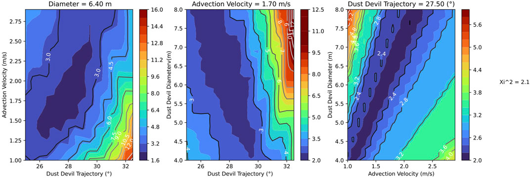
FIGURE 7. Contours of χ² in the θ_DD–v_DD space (left panel), θ_DD–d_DD space (central panel), and v_DD–d_DD space (right panel) for the solutions d_DD = 6.40 m, v_DD = 1.70 m s⁻¹, and θ_DD = 27.50°.

3.2.1 Dust devil trajectory from the cameras

Most DDs captured by the RDS were also recorded by the two commercial cameras operating during the campaign. Each camera has two fisheye lenses (one on either side of the camera) that can record full videos covering 360° in azimuth and 180° in elevation, with a resolution of 5.6 k (5,376 × 2,688 pixels) at a sampling rate of 30 frames per second. Because we do not have access to the raw data, we had to perform a pseudo-calibration. For doing that and assuming fisheye lenses are radially symmetric, we tried different relationships between the angle of incident light and where it is recorded on the camera sensor (e.g., stereographic, equisolid projections). By using the concentric circles made on the ground at 25, 50, and 75 m, we found that the equisolid projection is the most appropriate to relate the distance in pixels and the angle of incident light (each point on the circumference is at the same distance from the RDS, and thus, they should be at the same distance in pixels). With this relationship, we can project the DD trajectory derived in the previous section over the different images of the DD and, thus, validate the model retrievals. From different tests carried out after the campaign, we found that the errors in the estimation of these DD parameters using this approach are smaller than ∼6%. As indicated in the previous section, with the RDS observations, we can only obtain θ_DD and provide the relationship between v_DD and d_DD, which represents a family of DD trajectory solutions (straight-line trajectories) with the same slope but at different distances from the RDS. We can derive v_DD from the times and positions when the DD enters and leaves the 25-m concentric circle in the images, and from that, we can calculate d_DD using the relationship derived in the previous section (d_DD = 3.610⋅v_DD+0.0147). From this analysis, we obtain v_DD = 1.6 m s⁻¹ and d_DD = 5.8 m.

Once θ_DD, v_DD, and d_DD are known, we have a unique solution for the DD trajectory, whose projection over the camera images is shown in Figure 8. Here, the base of the DD follows the straight-line trajectory derived from the trajectory analysis quite well, highlighting the potential of the RDS observations to constrain not only the DD frequency of formation but also v_DD, θ_DD, and d_DD. The estimated v_DD and θ_DD were compared with the wind speed and direction measured by the Vaisala station (Figure 9). While v_DD is very similar to the values of the background wind speed measured around the detection, the wind direction is highly variable and different from the DD migration direction (θ_DD). From the data acquired during a terrestrial field campaign in the southwest United States of America, Balme et al. (2012) compared the background wind speed with the variation in the DD migration direction from the wind direction and found that the lower the ambient wind speed, the larger the deviation between these two direction components. If we compare the wind direction with θ_DD in the period between 3 min before and 3 min after the detection, then we get deviations that go from 0° up to $\sim 100°$, making the comparison difficult. Despite the low ambient wind speed and highly variable wind direction, the trajectory analysis indicates that, for this case, the DD trajectory is well represented by a straight line.

FIGURE 8

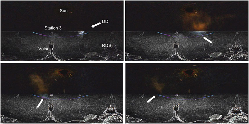
FIGURE 8. Color images of the DD detected on day 5 of the campaign (∼13:30 local time), along with the trajectory derived from the analysis of Section 3.2. The white arrow indicates the position of the DD.

FIGURE 9

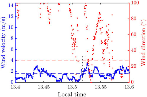
FIGURE 9. Comparison between the wind speed (blue dots) and direction (red dots) measurements with the derived parameters θ_DD (blue dashed line) and v_DD (red dashed line) for the DD encounter in Figure 8. The black dotted lines indicate the detection times of Lat-2, -8, and -7 sensors.

3.3 Dust lifting by wind gusts

In the previous section, it was demonstrated that by analyzing the detection timescales, we can differentiate the signal variations attributed to clouds and rather than DDs. However, from this parameter, we cannot automatically discriminate between a DD or a DL caused by wind gusts as both events have similar timescales (see Figure 6). Figure 10 shows two examples of DL events produced by wind gusts that were measured by the RDS on two different days of the campaign. These examples indicate that when the DL is registered by more than one channel, the time lag between detections is very short (or negligible) compared with that for a DD. This means that for the whole duration of an event detection (from the first detection up to the last one), the correlation between signals for a DL is much greater than for a DD. For instance, for the DL displayed in Figure 10A, we obtain a linear correlation coefficient (R²) between Lat-2 and Lat-3 signals of ∼0.54, while for Lat-2 and Lat-7 of the DD detection given in Figure 6B, R² is lower than 0.05. The main reason for these results lies in the differences between the DDs and the DL caused by wind gusts in terms of their dimensions. In contrast to the DDs, DL caused by wind gusts has a greater horizontal extension than it does vertically (see Figure 5). Because of this, a wind gust can cross the FOV of more than one Lat sensor almost simultaneously, which explains the different correlations between the DD detections (Figure 6) and wind gusts (Figure 10). Thus, for a dust event involving two or more Lat detections, we can determine if it is a DD or a DL by looking at the correlation between signals and the time lag between detections. The correlation criteria is very useful for cases where the DD passes in close proximity to the instrument; in such cases, the time lag between detections can be a few seconds.

FIGURE 10

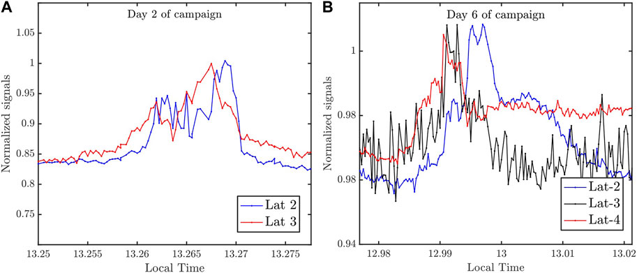
FIGURE 10. Two DL events produced by non-vortex wind gusts detected by the RDS on days 2 (A) and 6 (B) of the campaign. The smaller signal variations registered for the event of day 6 indicate a lower dust load. As for DDs, this is potentially due to the decrease in the amount of dust available on the surface following the rainy day. For each event, Lat detections are almost simultaneous and somewhat similar.

For the different DD and DL events detected by the RDS during the campaign, we found that the R² and time-lag criteria are robust enough to discriminate between these two events. As detailed in the following section, these results can be used for RDS observations on Mars. As pointed out by Newman et al. (2022), DL caused by wind gusts can cover an area several times larger than that of a DD, suggesting that both types of dust events could equally contribute to the dust budget of the planet during the non-storm period (depending on the frequency of formation). Although information on DL sizes from RDS observations is very limited, the high sampling frequency of MEDA (1 Hz) and its capability to operate for long periods allow us to constrain the diurnal, day-to-day, and seasonal variability of the frequency of formation of both of these events. From the analysis of the MEDA pressure observations, we can determine when a sequence of RDS detections is likely attributable to the presence of a DD (Hueso et al., 2022; Toledo et al., 2023). However, if the DD is far from the instrument, we can have cases in which the pressure measurements do not show a local pressure drop. Thus, in these cases, the values of R² between signals and the time lags between detections can provide key information to identify the event (as long as it has been registered in at least two Lat sensors).

Not all the dust events detected during the campaign were as easily identifiable (without the use of cameras) as those shown in Figures 6B, 10A. For example, in the case of the DL shown in Figure 10B, two simultaneous detections (for Lat-3 and 4) are observed, followed by a subsequent detection 3–4 s later by Lat-2. Through the videos recorded by the cameras, we could determine that the last detection was produced by the dust initially lifted during the first detection (by the Lat-3 and -4 sensors) and subsequently transported by the wind into the Lat-2 sensor’s FOV. That explains why the Lat-2 signal variation is not simultaneous with Lat-3 and -4 detections. For this reason, the correlation analysis should be carried out for any pair of detections, and if a correlation significantly different from zero (not necessarily for all of them) is observed, then the event is classified as a DL. For instance, in the case presented in Figure 10B, we found a correlation of 0.36 between Lat-3 and -4 detections, while the correlation between Lat-3 and Lat-2 detections is lower than 0.05.

Finally, there is a particular case in which the identification of the dust event can be complicated without the use of other instrumentation (e.g., pressure measurements) or further signal analyses. This is when a DD passes over the RDS such that it covers the FOV of different Lat sensors simultaneously. These DD encounters can be easily identified by combining the RDS with pressure measurements: if a local pressure drop is given at around the same time as the simultaneous detection, then the dust event is a DD. Otherwise (no local pressure drop), the dust event is a DL. If we do not have pressure measurements, a way to identify the event is also to look at the observations made by the Top sensors. If the simultaneous Lat detection is produced by a DD passing over the RDS, then the Top sensors should also display a detection at the same time. On the contrary, if simultaneous detection is produced by a DL, then, in general, the Top sensors should not display the sharp variation characteristic of when a DD completely covers the instrument. In general, the DL caused by wind gusts does not reach the heights of the DD, and thus, DL detections, as those shown in Figure 10, do not include significant variations by the Top sensors.

3.4 Comparison with RDS data on Mars

The results presented and discussed in the previous sections show the capability of the RDS to detect and characterize DDs. The following step in this work is to compare these DD detections with the RDS data on Mars and analyze the possible differences. These differences can arise from the following factors: i) DDs are, in general, larger in diameter and height on Mars (Balme and Greeley, 2006); ii) the different scattering properties of the Martian dust; and iii) the different conditions in the background aerosol optical depth (AOD) and Rayleigh scattering. Variations in the DD diameter and height (keeping constant the rest of the DD parameters) should result in different DD projections over the sensor’s FOV. As demonstrated by Toledo et al. (2023), these different projections yield different intensities in the DD detection (variation with respect to the background signal) but should, in principle, not change the shape of the detection. Figure 11A shows an example of DD detection performed by the RDS on Mars (on Sol 21 of the Mars 2020 mission). Similar to the campaign observations, the presence of the DD resulted in a signal increase for each of the RDS Lat sensors involved in the detection. We also observe that the sequence of detections is similar to those shown in Figures 2A, 6B. We made similar comparisons for other DD detections on Mars with the Lat sensors and found similar results. With respect to the Top sensor observations, Figure 11B shows an example of DD detection performed on Sol 313 (Top-1 and -7 signals are not displayed to facilitate the visualization). By comparing this detection with that shown in Figure 2, in both scenarios, the Top-8, -6, and -5 channels display a maximum. However, for Top-4 and -3 channels, the impact of the DD is different. On the other hand, in Figure 2B, we only see a minimum in the signals; for the Martian DD example, the minimum follows a maximum (a maximum that diminishes at shorter wavelengths).

FIGURE 11

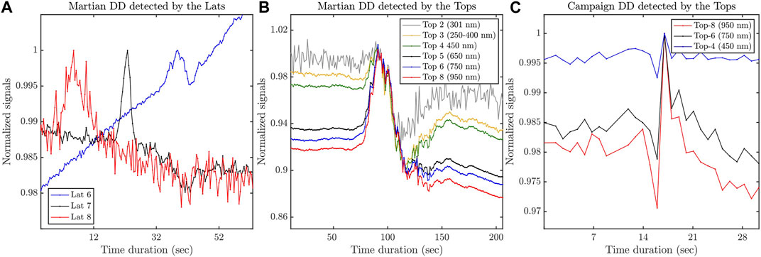
FIGURE 11. (A) DD detected by the RDS Lat sensors on Sol 21 of the mission (time of the detection ∼15:14 LTST). The DD produced increases to approximately 2.5, 8, and 7 W m⁻² in Lat-8, -7, and -6 sensors, respectively. (B) DD detected by the RDS Top sensors on Sol 313 of the mission (time of the detection ∼13:42 LTST). The minimum observed after the peak in the signals indicates that the DD affected the direct sunlight, or the light scattered at small scattering angles, received by the sensors. (C) RDS Top observations for the DD encounter of Figure 6 (day 5 of the campaign).

As discussed by Toledo et al. (2023), the net impact of the DD on the RDS Top observations depends, among other factors, on the DD and Sun angular positions. When DDs are at a position that affects the direct light or the forward scattering near the diffraction peak of the dust phase function, a decrease with respect to the background signals is expected at all the RDS wavelength bands. This was confirmed by the DD analyzed in Section 3.2 (Figures 6B, 8), for which the Top sensors also captured the event (see Figure 11C). Similar to the Martian case shown in Figure 11B, in Figure 11C, an increase and a decrease are observed during the encounter with the DD. From the DD trajectory derived from the camera videos and the trajectory analysis (see Figure 8), we know that the decrease in the signals is produced when the DD is affecting the direct light, or the light scattered at small scattering angles, received by the sensors. Therefore, it is very likely that the signal decrease observed in the DD case of Figure 11B is due to the same reasons. We examined several DD detections on Mars performed by the RDS Top sensors, and interestingly, we did not find cases similar to those shown in Figure 2B (maxima and minima occurring at the same time). The main reason is the impact of Rayleigh/molecular scattering in the terrestrial atmosphere (unlike the Martian dust particles, air molecules scatter the light equally at the forward and back scattering angles). In the Top-3 and -4 channels, the Rayleigh scattering contribution to the total sunlight received by the sensor is very important (e.g., scattering opacity at 450 nm ∼ 0.24). This means that, for the example shown in Figure 2B, the DD blocks the light scattered by the molecules in the Top-3 and -4 wavelength bands. In the other RDS wavelength bands, the Rayleigh opacity is much lower (e.g., at 650 ∼ 0.04), which explains why the signal decrease is not observed in the other channels on Earth (or in any of them on Mars, where the molecular scattering is negligible in all the wavelength bands).

The DL events caused by non-vortex winds observed during the campaign were also compared with cases detected on Mars. Figure 12 shows different dust events observed on Mars on sols 29, 64, 140, and 179. These cases could not be classified as DD by Toledo et al. (2023) because the pressure measurements did not show a local pressure drop and also because the Top sensors did not show any signal variations (the criteria followed in that work to classify a dust event as DD). By comparing these detections with the DL cases identified during the campaign (Figure 10), we clearly see that the events of sols 140 and 179 are DL caused by wind gusts. However, the dust events of sols 29 and 64 are complicated to classify. Although the sequence of detections is similar to that of a DD, the time lag between maxima (∼10 s) and the fact that the pressure sensor did not show a local minimum indicate that this event cannot be a DD. Indeed, for that short time period between maxima, the DD would have passed in close proximity to the RDS, and in such a scenario, the pressure sensor would have detected the vortex passage. For instance, for the DD event shown in Figure 11, the time between maxima was approximately 40 s, which indicates that the DD was far from the rover and explains the lack of pressure detection. A possibility for the events on sols 29 and 64 is that the wind gust only covered the FOV of the Lat sensor reporting the first detection (Lat 7), and then, the lifted dust particles were advected by the winds into the second Lat FOV (similar to what we observed in the example shown in Figure 10B). Another possibility is that the two detections are independent; e.g., they are produced by two distant DDs or two wind gusts. In any case, these dust events are difficult to classify and in general, only for the cases displaying a correlation between signals different from zero (Figure 10A,B), we can certainly confirm that they are produced by wind gusts.

FIGURE 12

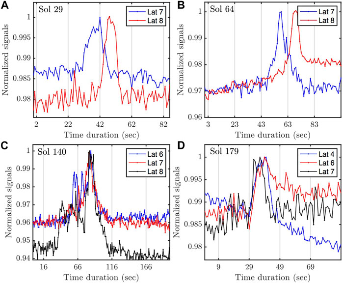
FIGURE 12. Dust events registered by the RDS Lat sensors on Mars for sols 29 (A), 64 (B), 140 (C) and 179 (D) of the mission. The correlation between signals indicates that the events shown in the lower panels are due to wind gusts.

3.5 Sampling frequency

In this section, we will discuss the impact of the instrument sampling frequency (f) on detecting DD and on deriving information about the DD trajectory, radius, and velocity (by performing the analysis described in Section 3.2). During the campaign, the RDS was operating at the same sampling frequency as on Mars (f = 1 Hz). However, SIS observations were acquired every 2 seconds (f = 0.5 Hz), which is the original configuration selected for the ExoMars 2022 mission (before it was suspended). These different configurations during the campaign allowed us to study what the optimal and minimum cadences required to detect and analyze DDs with this type of instrumentation are. When a DD crosses the FOV of one of the sensors, the number of observations involved in the detection mainly depends on 1) the instrument f and FOV; 2) the DD trajectory, v_DD and d_DD.

Figure 13 shows, as an example, two DDs detected by the SIS and RDS on day 5 of the campaign (the DD represented in the left panel is the same event as for the analysis in Section 3.2; see Figure 6B). For both instruments, the angular aperture of the Lat sensors is the same (±5°). Here, the limitations of SIS sampling frequency for detecting DDs are as follows: for Lat-3 and Lat-4, the number of observations involved in the detection is very limited (just one observation per channel). If, in this event, the Lat-2 had not been involved in the detection, then it would have been difficult to interpret these observations and confirm the detection of a DD. It is true that, in this particular case, the DD was formed very near the SIS (25 m away from the RDS), and this could explain the simultaneous increases of channels Lat-2 and -3. However, for the other example of DD detection (Figure 13B), we see again only one SIS observation that is significantly above the background signal (as a result of the DD). Even if the DD had been detected by another SIS Lat sensor, confirming its presence would have been challenging (unless we had additional complementary instrumentation, such as a pressure sensor).

FIGURE 13

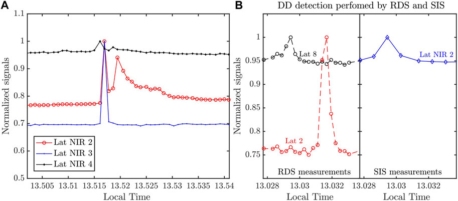
FIGURE 13. Examples of DD detections performed by SIS and RDS Lat sensors. The example in (A) is the same event analyzed in Figure 8 (day 5 of the campaign). For the DD encounter of (B) only one of the SIS Lat sensors captured the event.

Although in other DD events during the campaign, the SIS sampling frequency was enough, in some other cases, such as those illustrated in Figure 13, it was not enough. This implies that if the SIS and RDS were operating at two different locations but with the same DD frequency of formation (the number of DDs formed per unit of area and time, ρ_DD), the RDS would detect more DDs than the SIS, and thus, we would derive different values of ρ_DD. In order to study the impact of f on the detection of DDs, we performed several numerical simulations. In these simulations, we start with an a priori DD frequency of formation, and several DDs are formed randomly within an area A_max = $\pi \cdot {\mathrm{d}}_{\max }^2$, whose initial positions are given as follows:

$\mathrm{x}={\mathrm{d}}_{\max }\times \sqrt{r}\times \cos (\mathrm{\Theta }),(3)$

$\mathrm{y}={\mathrm{d}}_{\max }\times \sqrt{r}\times \sin (\mathrm{\Theta }),(4)$

where r and Θ are uniformly distributed variables (r ∈ [0,1] and Θ ∈ [0,2π) and d_max is the maximum distance at which a DD can be formed in the model. The square root of r is used to have the same number of points per unit of area. Once a DD is generated, it travels a distance d = v_DD ⋅t_DD, assuming a straight line. The left panel of Figure 14 shows a schematic of the model: the red dots indicate the initial position of the DDs, and the black dots indicate the trajectories (the number of dots is equal to t_DD/f, where f is the sampling frequency). A detection is made if the DD crosses the FOV of the sensor for at least three observations. That is to say, if the part of the trajectory that crosses the FOV contains at least three black dots (for the diagram in Figure 14), this condition is met for only 1 DD. See the work of Toledo et al. (2023) for a complete description of the model. The right panel of Figure 14 shows the variation of the number of DD detections (n_DD) with the sampling frequency for a Lat sensor and for two different angles between the DD trajectory and the azimuth orientation of the sensor (θ). The number of detections was normalized by the value of n_DD for f = 5 Hz. These simulations indicate that for f = 1 Hz and 0.5 Hz, most of the DDs that cross the Lat sensor are detected (variations with respect to n_DD for f = 5 Hz are lower than 8% and 15%, respectively). However, for f smaller than 0.33 Hz–0.50 Hz, the differences with respect to the ideal case can be important (greater than 20%–25%) and lead to noticeable errors in the estimation of ρ_DD.In the latter case, however, a correction can be applied to the measured n_DD based on the sampling frequency of the instrument and the simulations shown in Figure 14. It should be noted that this correction depends significantly on the DD trajectory for sampling frequencies below 1 Hz. Indeed, while the normalized DD detections for θ = 0° and = 45° are quite similar for f = 1 Hz, we observe noticeable deviations for smaller values of f = 1 Hz. As information on the DD trajectory (θ) is limited for the cases when the DD does not cross more than one sensor FOV, we conclude that a sampling frequency of 1 Hz is adequate for assessing the DD density of formation from the RDS or SIS observations.

FIGURE 14

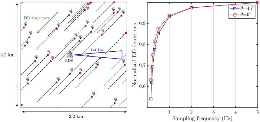
FIGURE 14. Schematic of the RDS detections (for a Lat sensor) for a constant DD frequency of formation, advection velocity, and trajectory (left). The initial position of the DD trajectory is indicated by the red dots, and the trajectory length is given by t_DD and v_DD. A detection is only accounted for if the DD trajectory crosses the sensor FOV (delimited by the solid blue line) and for at least three sensor observations (defined by the sampling frequency). Variation in the number of sensor detections (n_DD) with the sampling frequency for two different DD trajectories (right). All the n_DD values were normalized by the number of sensor detections when f = 5 Hz.

Finally, we studied the impact of the sampling frequency on the DD trajectory analysis of Section 3.2. The same trajectory analysis as shown in Figure 7 was performed using only the RDS observations collected every 2 seconds (f = 0.5 Hz), whose results are displayed in Figure 15. For comparison purposes, the original results (f = 1 Hz) are also shown. Although the derived DD trajectory is not very affected for f = 0.5 Hz, for the DD diameter and advection velocity relationship, some significant differences are observed. If we assume the DD migration velocity derived from the images (v_DD = 1.6 m s⁻¹), then the differences in d_DD are approximately 33%. Thus, these results indicate that for sampling frequencies lower than ∼ 1 Hz, the capability of the RDS to detect and characterize DD is highly limited.

FIGURE 15

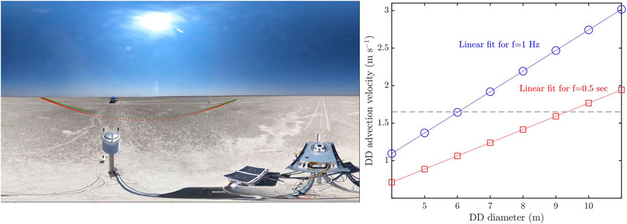
FIGURE 15. DD trajectories (left panel) and linear relationships between the DD diameter and advection velocity (right panel) derived for the DD encounter of Figure 6 using two different sampling frequencies (f): f = 1 and 0.5 Hz. The red and green dots in the left panel represent the DD trajectories for f = 1 Hz and 0.5 Hz, respectively.

4 Conclusion

In this paper, we analyzed the RDS observations collected during a field campaign conducted from 29 September to 6 October 2021 in the Makgadikgadi Salt Pans (Botswana). The main goal of the campaign was to study the capabilities of the RDS to detect DDs and DL caused by non-vortex wind gusts. We reached the following main conclusions:

1. We demonstrated that the RDS is a reliable instrument for the detection and characterization of DDs. During the campaign, several DD encounters detected by the RDS were recorded using the cameras, and from that, we could validate the different models used to detect and constrain the DD properties on Mars. In DD encounters involving more than one Lat detection, the DD migration speed and direction, as well as the diameter, can be constrained. The DD migration speed and diameter can only be constrained by a linear relationship that can be resolved with data from other instruments (such as pressure measurements). As expected, the number of DDs detected by the cameras was higher than the detections carried out by the RDS (by a factor of 8). However, the potential of the RDS (or similar instrumentation) is its low power consumption and data volume, which allow it to operate on Mars for longer periods of time and at a higher sampling frequency than the cameras.

2. The signal variations produced by other factors such as clouds or wind gusts can be filtered out by looking at the timescale of the signatures or the correlation between the signals involved in the detection. For clouds, the timescales are about 10 times longer and the variations are smoother. For DL caused by wind gusts, although the timescale of the detections is comparable to that of DDs, the correlation of the signals involved in the detection is significantly different than zero (contrary to the DD detections). This is due to its greater horizontal extension, which can cover more than one Lat sensor FOV simultaneously (or almost simultaneously). If the dust event is only detected in one Lat sensor, then we cannot determine if it is a DD or a DL caused by a wind gust.

3. The comparison between the Earth and Martian RDS observations shows that DD and DL events have a similar impact on the RDS. The only differences observed are for the Top sensors, whose spectral bands are significantly affected by Rayleigh scattering. Therefore, the Makgadikgadi Salt Pans are a good analog for Martian DD investigations.

4. The sampling frequency (f) of the instrument is a critical parameter for the study of DDs with this type of instrumentation. First, f has an impact on the number of DDs detected. If f is decreased to 0.3 Hz or more, then more than 20%–24% of the DDs crossing the FOV of the sensors will not be detected. Thus, this can result in large errors in the estimation of the DD frequency of formation (the number of DDs per unit area and time). In addition, increasing f also results in large errors in the estimation of the DD diameter and advection velocity. For example, a decrease in f from 1 Hz to 0.5 Hz leads to errors of approximately 33% in the estimation of the DD diameter.

Finally, this work shows the importance of field campaigns in Martian analogs to characterize the potential of the observations made by RDS-type instrumentation. The high place-to-place and temporal variability of the DD properties on Mars requires continuous DD observations at different locations to really constrain their contribution to the global atmospheric dust budget of the planet. In this regard, observations from the SIS that was part of the ExoMars 2022 lander could have provided information about DDs at a new location and, thus, new data for the validation of the theoretical dust-cycle models. In future field campaigns in terrestrial analogs, we plan to evaluate the use of simpler sensors, such as the SIS’16 (Arruego et al., 2017; Toledo et al., 2017) that was part of the DREAMS Experiment on board the ExoMars 2016 mission (Esposito et al., 2018) or the Optical Depth Sensor (ODS) (Toledo et al., 2016b; Toledo et al., 2016a), to constrain the DD properties. Indeed, these light, small, and low-energy-consumption sensors can be easily installed on small stations on board probes or rovers, and thus, they are a good option for future missions with limited energy and transmission resources.

Data availability statement

The datasets presented in this study can be found in online repositories. The names of the repository/repositories, accession number(s), and the data of some of the figures can be found at: https://doi.org/10.5281/zenodo.7930641; all perseverance data used in this study are publicly available via the Planetary Data System (2021; Rodriguez-Manfredi et al., 2021).

Author contributions

DT: Conceptualization, Data curation, Formal analysis, Funding acquisition, Investigation, Methodology, Software, Supervision, Validation, Visualization, Writing—original draft and Writing—review & editing. VA: Conceptualization, Data curation, Formal analysis, Funding acquisition, Investigation, Methodology, Software, Validation, Visualization, Writing—original draft and Writing—review & editing JM-O: Investigation, Data curation, Formal analysis, Visualization. FF: Investigation, Visualization, Writing—original draft and Writing—review & editing. FS: Investigation, Data curation, Formal analysis, Visualization. MY: Investigation, Data curation, Formal analysis, Visualization. MT: Investigation, Data curation, Visualization, Project administration, Funding acquisition. JR-M: Investigation, Data curation, Project administration, Funding acquisition. IA: Investigation, Data curation, Formal analysis, Visualization, Project administration, unding acquisition.

Funding

This research was carried out under research permit CMLWS 1/17/4 II (28), granted to FF, by the Ministry of Land Management, Water, and Sanitation Services, Government of Botswana. The field work and research was funded by 1) Europlanet 2024 transnational access. Europlanet 2024 RI received funding from the European Union’s Horizon 2020 Research and Innovation Programme under grant agreement number 871149; 2) the Spanish Ministry of Economy and Competitiveness, through project nos. ESP2014-54256-C4-1-R (also -2-R, -3-R, and -4-R); 3) the Ministry of Science, Innovation, and Universities, project nos. ESP2016-79612-C3-1-R (also -2-R and -3-R); and 4) the Ministry of Science and Innovation/State Agency of Research (10.13039/501100011033), project nos. ESP2016-80320-C2-1-R, RTI 2018-098728-B-C31 (also -C32 and -C33), and RTI 2018-099825-B-C31.

Conflict of interest

The authors declare that the research was conducted in the absence of any commercial or financial relationships that could be construed as a potential conflict of interest.

Publisher’s note

All claims expressed in this article are solely those of the authors and do not necessarily represent those of their affiliated organizations, or those of the publisher, the editors, and the reviewers. Any product that may be evaluated in this article, or claim that may be made by its manufacturer, is not guaranteed or endorsed by the publisher.

References

Almansa, A. F., Cuevas, E., Torres, B., Barreto, Á., García, R. D., Cachorro, V. E., et al. (2017). A new zenith-looking narrow-band radiometer-based system (zen) for dust aerosol optical depth monitoring. Atmos. Meas. Tech. 10, 565–579. doi:10.5194/amt-10-565-2017

CrossRef Full Text | Google Scholar

Apestigue, V., Gonzalo, A., Jiménez, J. J., Boland, J., Lemmon, M., de Mingo, J. R., et al. (2022). Radiation and dust sensor for mars environmental dynamic analyzer onboard m2020 rover. Sensors 22, 2907. doi:10.3390/s22082907

PubMed Abstract | CrossRef Full Text | Google Scholar

Apestigue, V., Toledo, D., Arruego, I., Smith, M. D., Lemmon, M., Gómez, L., et al. (2021). Dust devils detection and characterization at jezero using meda radiance observations. AAS/Division Planet. Sci. Meet. Abstr. 53, 203–207.

Google Scholar

Arruego, I., Apéstigue, V., Jiménez-Martín, J., Martínez-Oter, J., Álvarez-Ríos, F., González-Guerrero, M., et al. (2017). Dreams-sis: the solar irradiance sensor on-board the exomars 2016 lander. Adv. Space Res. 60, 103–120. doi:10.1016/j.asr.2017.04.002

CrossRef Full Text | Google Scholar

Arruego, I., López, F., Saiz, A., Sánchez, A., Yela, M., Martínez, J., et al. (2016). “Sun irradiance and dust sensor investigations on board the exomars 2018 lander,” in 13th international planetary probe workshop (13th IPPW) (Washington, DC, Maryland: IPPW).

Google Scholar

Balme, M., and Greeley, R. (2006). Dust devils on earth and mars. Rev. Geophys. 44. doi:10.1029/2005rg000188

CrossRef Full Text | Google Scholar

Balme, M., Pathare, A., Metzger, S., Towner, M., Lewis, S., Spiga, A., et al. (2012). Field measurements of horizontal forward motion velocities of terrestrial dust devils: towards a proxy for ambient winds on mars and earth. Icarus 221, 632–645. doi:10.1016/j.icarus.2012.08.021

CrossRef Full Text | Google Scholar

Basu, S., Richardson, M. I., and Wilson, R. J. (2004). Simulation of the martian dust cycle with the gfdl mars gcm. J. Geophys. Res. Planets 109, E11006. doi:10.1029/2004je002243

CrossRef Full Text | Google Scholar

Changela, H. G., Chatzitheodoridis, E., Antunes, A., Beaty, D., Bouw, K., Bridges, J. C., et al. (2021). Mars: new insights and unresolved questions. Int. J. Astrobiol. 20, 394–426. doi:10.1017/s1473550421000276

CrossRef Full Text | Google Scholar

Esposito, F., Debei, S., Bettanini, C., Molfese, C., Arruego Rodríguez, I., Colombatti, G., et al. (2018). The dreams experiment onboard the schiaparelli module of the exomars 2016 mission: design, performances and expected results. Space Sci. Rev. 214, 103–138. doi:10.1007/s11214-018-0535-0

CrossRef Full Text | Google Scholar

Farrell, W., Smith, P., Delory, G., Hillard, G., Marshall, J., Catling, D., et al. (2004). Electric and magnetic signatures of dust devils from the 2000–2001 matador desert tests. J. Geophys. Res. Planets 109, E03004. doi:10.1029/2003je002088

CrossRef Full Text | Google Scholar

Fenton, L. K., and Lorenz, R. (2015). Dust devil height and spacing with relation to the martian planetary boundary layer thickness. Icarus 260, 246–262. doi:10.1016/j.icarus.2015.07.028

CrossRef Full Text | Google Scholar

Ferri, F., Smith, P. H., Lemmon, M., and Rennó, N. O. (2003). Dust devils as observed by mars pathfinder. J. Geophys. Res. Planets 108, 1421. doi:10.1029/2000je001421

CrossRef Full Text | Google Scholar

Fisher, J. A., Richardson, M. I., Newman, C. E., Szwast, M. A., Graf, C., Basu, S., et al. (2005). A survey of martian dust devil activity using mars global surveyor mars orbiter camera images. J. Geophys. Res. Planets 110, 2165. doi:10.1029/2003je002165

CrossRef Full Text | Google Scholar

Franchi, F., Cavalazzi, B., Evans, M., Filippidou, S., Mackay, R., Malaspina, P., et al. (2022). Late pleistocene–holocene palaeoenvironmental evolution of the makgadikgadi basin, central kalahari, Botswana: new evidence from shallow sediments and ostracod fauna. Front. Ecol. Evol. 10, 818417. doi:10.3389/fevo.2022.818417

CrossRef Full Text | Google Scholar

Franchi, F., MacKay, R., Selepeng, A. T., and Barbieri, R. (2020). Layered mound, inverted channels and polygonal fractures from the makgadikgadi pan (Botswana): possible analogues for martian aqueous morphologies. Planet. Space Sci. 192, 105048. doi:10.1016/j.pss.2020.105048

CrossRef Full Text | Google Scholar

Greeley, R., Whelley, P. L., Arvidson, R. E., Cabrol, N. A., Foley, D. J., Franklin, B. J., et al. (2006). Active dust devils in gusev crater, mars: observations from the mars exploration rover spirit. J. Geophys. Res. Planets 111, 2743. doi:10.1029/2006je002743

CrossRef Full Text | Google Scholar

Hargitai, H., and Kereszturi, Á. (2015). Encyclopedia of planetary landforms. New York, NY: Springer.

Google Scholar

Hueso, R., Newman, C., Río-Gaztelurrutia, T. d., Munguira, A., Sánchez-Lavega, A., Toledo, D., et al. (2022). Convective vortices and dust devils detected and characterized by mars 2020. J. Geophys. Res. Planets 128, e2022JE007516. doi:10.1029/2022JE007516

CrossRef Full Text | Google Scholar

Jackson, B. (2022). Vortices and dust devils as observed by the mars environmental dynamics analyzer instruments on board the mars 2020 perseverance rover. Planet. Sci. J. 3, 20. doi:10.3847/psj/ac4586

CrossRef Full Text | Google Scholar

Kahanpää, H., and Viúdez-Moreiras, D. (2021). Modelling martian dust devils using in-situ wind, pressure, and uv radiation measurements by mars science laboratory. Icarus 359, 114207. doi:10.1016/j.icarus.2020.114207

CrossRef Full Text | Google Scholar

Kahre, M. A., Murphy, J. R., and Haberle, R. M. (2006). Modeling the martian dust cycle and surface dust reservoirs with the nasa ames general circulation model. J. Geophys. Res. Planets 111, E06008. doi:10.1029/2005je002588

CrossRef Full Text | Google Scholar

Lorenz, R. D. (2016). Heuristic estimation of dust devil vortex parameters and trajectories from single-station meteorological observations: application to insight at mars. Icarus 271, 326–337. doi:10.1016/j.icarus.2016.02.001

PubMed Abstract | CrossRef Full Text | Google Scholar

Lorenz, R. D., and Jackson, B. K. (2015). Dust devils and dustless vortices on a desert playa observed with surface pressure and solar flux logging. GeoResJ 5, 1–11. doi:10.1016/j.grj.2014.11.002

CrossRef Full Text | Google Scholar

Lorenz, R. D., Lemmon, M. T., and Maki, J. (2021). First mars year of observations with the insight solar arrays: winds, dust devil shadows, and dust accumulation. Icarus 364, 114468. doi:10.1016/j.icarus.2021.114468

CrossRef Full Text | Google Scholar

Lorenz, R. (2012). Observing desert dust devils with a pressure logger. Geoscientific Instrum. Methods Data Syst. 1, 209–220. doi:10.5194/gi-1-209-2012

CrossRef Full Text | Google Scholar

Lorenz, R. (2013). The longevity and aspect ratio of dust devils: effects on detection efficiencies and comparison of landed and orbital imaging at mars. Icarus 226, 964–970. doi:10.1016/j.icarus.2013.06.031

CrossRef Full Text | Google Scholar

Martínez, G. M., Sebastián, E., Vicente-Retortillo, A., Smith, M. D., Johnson, J. R., Fischer, E., et al. (2023). Surface energy budget, albedo, and thermal inertia at jezero crater, mars, as observed from the mars 2020 meda instrument. J. Geophys. Res. Planets 128, e2022JE007537. doi:10.1029/2022je007537

CrossRef Full Text | Google Scholar

Metzger, S. M., Carr, J. R., Johnson, J. R., Parker, T. J., and Lemmon, M. T. (1999). Dust devil vortices seen by the mars pathfinder camera. Geophys. Res. Lett. 26, 2781–2784. doi:10.1029/1999gl008341

CrossRef Full Text | Google Scholar

Newman, C. E., Hueso, R., Lemmon, M. T., Munguira, A., Vicente-Retortillo, Á., Apestigue, V., et al. (2022). The dynamic atmospheric and aeolian environment of jezero crater, mars. Sci. Adv. 8, eabn3783. doi:10.1126/sciadv.abn3783

PubMed Abstract | CrossRef Full Text | Google Scholar

Newman, C. E., Lewis, S. R., Read, P. L., and Forget, F. (2002). Modeling the martian dust cycle 2. multiannual radiatively active dust transport simulations. J. Geophys. Res. Planets 107, 7-1–7-15. doi:10.1029/2002je001920

CrossRef Full Text | Google Scholar

Oke, A., Tapper, N. J., and Dunkerley, D. (2007). Willy-willies in the australian landscape: the role of key meteorological variables and surface conditions in defining frequency and spatial characteristics. J. arid Environ. 71, 201–215. doi:10.1016/j.jaridenv.2007.03.008

CrossRef Full Text | Google Scholar

Ordóñez-Etxeberria, I., Hueso, R., and Sánchez-Lavega, A. (2020). Strong increase in dust devil activity at gale crater on the third year of the msl mission and suppression during the 2018 global dust storm. Icarus 347, 113814. doi:10.1016/j.icarus.2020.113814

CrossRef Full Text | Google Scholar

Pál, B., and Kereszturi, Á. (2020). Annual and daily ideal periods for deliquescence at the landing site of insight based on gcm model calculations. Icarus 340, 113639. doi:10.1016/j.icarus.2020.113639

CrossRef Full Text | Google Scholar

Perrin, C., Rodriguez, S., Jacob, A., Lucas, A., Spiga, A., Murdoch, N., et al. (2020). Monitoring of dust devil tracks around the insight landing site, mars, and comparison with in situ atmospheric data. Geophys. Res. Lett. 47, e2020GL087234. doi:10.1029/2020gl087234

CrossRef Full Text | Google Scholar

Reiss, D., Fenton, L., Neakrase, L., Zimmerman, M., Statella, T., Whelley, P., et al. (2016). Dust devil tracks. Space Sci. Rev. 203, 143–181. doi:10.1007/s11214-016-0308-6

CrossRef Full Text | Google Scholar

Rodriguez-Manfredi, J. A., De la Torre Juárez, M., Alonso, A., Apéstigue, V., Arruego, I., Atienza, T., et al. (2021). The mars environmental dynamics analyzer, meda. a suite of environmental sensors for the mars 2020 mission. Space Sci. Rev. 217, 1–86. doi:10.1007/s11214-021-00816-9

CrossRef Full Text | Google Scholar

Rodriguez-Manfredi, J., de la Torre Juarez, M., Sanchez-Lavega, A., Hueso, R., Martinez, G., Lemmon, M., et al. (2023). The diverse meteorology of jezero crater over the first 250 sols of perseverance on mars. Nat. Geosci. 16, 19–28. doi:10.1038/s41561-022-01084-0

CrossRef Full Text | Google Scholar

Schmidt, G., Franchi, F., Salvini, F., Selepeng, A. T., Luzzi, E., Schmidt, C., et al. (2023a). Fault controlled geometries by inherited tectonic texture at the southern end of the east african rift system in the makgadikgadi basin, northeastern Botswana. Tectonophysics 846, 229678. doi:10.1016/j.tecto.2022.229678

CrossRef Full Text | Google Scholar

Schmidt, G., Luzzi, E., Franchi, F., Selepeng, A., Hlabano, K., and Salvini, F. (2023b). Structural influences on groundwater circulation in the makgadikgadi salt pans of Botswana? Implications for martian playa environments. Front. Astronomy Space Sci. 10, 1108386. doi:10.3389/fspas.2023.1108386

CrossRef Full Text | Google Scholar

Serrano, F., Oter, J. M., Apestigue, V., Nuñez, J., Montalbo, S., de Mingo, J. R., et al. (2022). “I-Box: an automated remote sensing system for space scientific instrumentation,” in 2022 IEEE 9th International Workshop on Metrology for AeroSpace (MetroAeroSpace), Pisa, Italy, 27-29 June 2022 (IEEE), 526–531.

CrossRef Full Text | Google Scholar

Sinclair, P. C. (1973). The lower structure of dust devils. J. Atmos. Sci. 30, 1599–1619. doi:10.1175/1520-0469(1973)030<1599:tlsodd>2.0.co;2

CrossRef Full Text | Google Scholar

Thomas, P., and Gierasch, P. J. (1985). Dust devils on mars. Science 230, 175–177. doi:10.1126/science.230.4722.175

PubMed Abstract | CrossRef Full Text | Google Scholar

Toledo, D., Apéstigue, V., Arruego, I., Lemmon, M., Gómez, L., Montoro, A. D. F., et al. (2023). Dust devil frequency of occurrence and radiative effects at jezero crater, mars, as measured by meda radiation and dust sensor (rds). J. Geophys. Res. Planets 128, 7494. doi:10.1029/2022je007494

CrossRef Full Text | Google Scholar

Toledo, D., Arruego, I., Apéstigue, V., Jiménez, J., Gómez, L., Yela, M., et al. (2017). Measurement of dust optical depth using the solar irradiance sensor (sis) onboard the exomars 2016 edm. Planet. Space Sci. 138, 33–43. doi:10.1016/j.pss.2017.01.015

CrossRef Full Text | Google Scholar

Toledo, D., Rannou, P., Pommereau, J. P., and Foujols, T. (2016a). The optical depth sensor (ods) for column dust opacity measurements and cloud detection on martian atmosphere. Exp. Astron. 42, 61–83. doi:10.1007/s10686-016-9500-7

CrossRef Full Text | Google Scholar

Toledo, D., Rannou, P., Pommereau, J. P., Sarkissian, A., and Foujols, T. (2016b). Measurement of aerosol optical depth and sub-visual cloud detection using the optical depth sensor (ods). Atmos. Meas. Tech. 9, 455–467. doi:10.5194/amt-9-455-2016

CrossRef Full Text | Google Scholar

Verba, C. A., Geissler, P. E., Titus, T. N., and Waller, D. (2010). Observations from the high resolution imaging science experiment (hirise): martian dust devils in gusev and russell craters. J. Geophys. Res. Planets 115, E09002. doi:10.1029/2009je003498

CrossRef Full Text | Google Scholar

Vicente-Retortillo, A., Martínez, G. M., Lemmon, M. T., Hueso, R., Johnson, J., Sullivan, R., et al. (2023). Dust lifting through surface albedo changes at jezero crater, mars. J. Geophys. Res. Planets 128, e2022JE007672. doi:10.1029/2022je007672

CrossRef Full Text | Google Scholar