Quantifying the ability of magnetohydrodynamic models to reproduce observed Birkeland current and auroral electrojet magnitudes

Although global magnetohydrodynamic (MHD) models have increased in sophistication and are now at the forefront of modeling Space Weather, there is still no clear understanding of how well these models replicate the observed ionospheric current systems. Without a full understanding and treatment of the ionospheric current systems, global models will have significant shortcomings that will limit their use. In this study we focus on reproducing observed seasonal interhemispheric asymmetry in ionospheric currents using the Space Weather Modeling Framework (SWMF). We find that SWMF does reproduce the linear relationship between the electrojets and the FACs, despite the underestimation of the currents’ magnitudes. Quantitatively, we find that at best SWMF is only capturing approximately 60% of the observed current. We also investigate how varying F10.7 effects the ionospheric potential and currents during the summer and winter. We find that simulations ran with higher F10.7 result in lower ionospheric potentials. Additionally, we find that the models do not always replicate the expected behavior of the currents with varying F10.7. This work points to a needed improvement in ionospheric conductance models.

1 Introduction

To better understand the dynamics of the interactions that contribute to space weather and to predict their effects, scientists must analyze the underlying physics that contribute, through observations and model validation. As a result of southward interplanetary magnetic field (IMF) merging with the geomagnetic field on the day side, magnetic reconnection occurs on the night side and subsequently transfers solar wind energy to the magnetosphere and ionosphere (Dungey, 1961). In the ionosphere, the motion of the plasma produced by the solar wind-magnetosphere interaction means that, in the frame of Earth, there is an electric field and voltage across the ionosphere from dawn to dusk. This voltage is directly proportional to the solar wind electric field as long as the solar wind mach number is large (Lopez et al., 2010). However, there are several factors that contribute to interhemispheric asymmetries in the transpolar potential, ionospheric conductivity, density, and more that result from this interaction: different amounts of sunlight, unequal particle precipitation, the offset in the magnetic poles, even different wind patterns (Laundal et al., 2017). Without a full understanding and treatment of these asymmetries, global models will have clear shortcomings that will limit their use. Traditionally, Magnetohydrodynamic (MHD) based global simulations have been at the forefront of modeling the Sun-Earth environment and the dynamics thereof. However, the extent to which these MHD models incorporate and accurately represent interhemispheric asymmetries are unknown. What is known is that these models treat the Northern and Southern Hemispheres the same. The domains of these models range from the inner heliosphere to Earth’s thermosphere. There are four global magnetosphere MHD-based models are available to the community through the Community Coordinated Modeling Center (CCMC): the Open Geospace General Circulation Model (Open GGCM) (Raeder et al., 2009), the Lyon-Fedder-Mobarry model (LFM) (Lyon et al., 2004), the Grand Unified Magnetosphere Ionosphere Coupling Simulation (GUMICS) (Janhunen et al., 2012), and Space Weather Modeling Framework (SWMF) (Tóth et al., 2005). Though these models are readily accessible, their capabilities to accurately model the global environment and reproduce observations are actively being validated within the space weather community (Gordeev et al., 2015; Mukhopadhyay, 2022; Honkonen et al., 2013; Gordeev et al., 2015 evaluate the four first-principle magnetospheric models ability to replicate basic magnetospheric global variables realistically, as given by published empirical relationship of these variables. The authors have concluded that these models do a reasonable job at replicating magnetospheric size, magnetic field, and pressure, but there is variation amongst the four models on their performance in predicting the global convection rate, total field-aligned current, and magnetic flux loading into the magnetotail during substorms.

The need for model validation of currents and geomagnetic disturbances has been addressed by community-wide space weather model validation efforts lead by the Geospace Environment Modeling (GEM) Metric and Validation Focus Groups (Pulkkinen et al., 2013; Glocer et al., 2016). However, these studies only looked to validate models at ground magnetometer station locations. We still do not have a comprehensive survey of how well the codes are reproducing observed currents patterns and magnitudes of ionospheric electrojets and Birkeland currents.

James and Lopez (2022) work focus on the asymmetries in ionospheric conductivity that ultimately controls the amount of current that is allowed to be closed through the conductive ionosphere. During the summer, the northern polar region is tilted towards the Sun and therefore receives more sunlight in which in return further ionizes the ionosphere, making it more conductive. However, during the winter, the same polar region is tilted away from the Sun, receiving less sunlight, and therefore becomes less conductive. The authors find this rationale to hold qualitatively, using observations. They find there to be larger field-aligned currents flowing into and eastward and westward electrojets in the ionosphere during the summer than during the winter. Secondly, the authors determined the relationship between the electrojets and Birkeland current. Lastly, in investigating the role F10.7 plays in relation to the magnitude of current in the ionosphere, the author’s determined that as F10.7 increases during the winter, the magnitude of the currents decreases.

In this work, we quantify the ability of MHD models to reproduce the observed asymmetries in ionospheric currents presented in James and Lopez (2022).

2 Methodology

In this section we first provide an overview of the data and observations used. We then include a brief description of the Space Weather Modeling Framework (SWMF) and justification for events and data used in this study.

2.1 Data and observations

We conduct this study to validate the ability of global MHD models to reproduce ionospheric current magnitudes using observational Birkeland Current data provided by the Active Magnetosphere and Planetary Response Experiment (AMPERE) dataset and observational electrojet strength as quantified by the SuperMag Electrojet index (SME) from the SuperMag dataset. The AMPERE dataset (https://ampere.jhuapl.edu) consists of data from over 66 LEO satellites that are apart of the Iridium constellation. Theses satellites are equipped with magnetometers whose data are then used to make global maps of Birkeland currents (Anderson et al., 2000; Waters et al., 2001). The Birkeland current data products are expressed in 2-min increments. The SuperMag data are collected and derived as described in Gjerloev (2012). The SuperMag Electrojet index (SME) is used in this study as a measure for the auroral electrojet activity. Typically the AE index is used as a measure of auroral electrojet activity. However, in this study we use the SuperMag Electrojet index (SME). SME is derived in the same way that AE is. However, SME use over 150 stations while AE use about 12 stations and thus is a more global measure of the electrojets. The magnitude of the electrojets are indexed by finding the largest northward or southward perturbation from ground magnetometers. AU or SMU is the largest northward perturbation indicating the largest eastward electrojet. AL or SML is largest southward perturbation indicating the largest westward electrojet and AE or SME is determined by subtracting AL form AU.

The simulated data is provided by SWMF output. We run several SWMF simulations using CCMC’s runs-on-request feature. The model output is made publicly available, once the run is finished. AE and Birkeland current are standard output parameters for these runs, in 1 min increments. SME, however is not. In this study, the simulated SME is calculated independently using the ground magnetometer data from the models, in the same way the observational SME is derived.

The AMPERE Birkeland current data are provided in 2 min intervals, therefore all data sets used in comparison to the observational Birkeland current are averaged every 2-min.

2.2 Model description

The SWMF integrates nine numerical models: the Solar Corona, Solar Eruption Generator, Inner Heliosphere, Solar Energetic Particles, Global Magnetosphere, Inner Magnetosphere, Radiation Belt, Ionospheric Electrodynamics, and Upper Atmosphere and Ionosphere, into one coherent model (Tóth et al., 2005). Each domain or model exchanges information with one another to simulate the real world dynamics of the system interactions. The Global Magnetosphere (GM) includes the planet’s bow shock, magnetopause, and magnetotail. The physics of this domain is approximated by solving the resistive MHD equations and using the Block-Adaptive-Tree-Solarwind-Roe-Upwind-Scheme (BATS-R-US). BATS-R-US is typically restricted to the domain 2.5R_E from the center of Earth and expands to about 30R_E on the dayside, hundreds of R_E on the night side, and 50–100R_E in the directions orthogonal to the Sun-Earth line. The domain inside 2.5R_E is approximated by the Inner Magnetosphere (IM), Radiation Belt (RB), and Ionosphere Electrodynamics (IE) components of the SWMF model. There are several options in SWMF for the IM component, but in this study we focus on events where the Rice Convection Model (RCM) (De Zeeuw et al., 2001; Toffoletto et al., 2003) is used to calculate the distribution function of the ring current ions and electrons given an electric and magnetic field distribution. The RCM self consistently computes field-aligned currents and potentials. There are other codes that have been developed to preform similarly (e.g., the Comprehensive Inner-Magnetosphere Ionosphere (CIMI) Model; Fok et al., 2014).

In the, IE component, the Ridley Ionosphere Model (RIM) works as a height averaged electric potential solver, which uses the field-aligned currents from GM and Upper Atmosphere (UA) to calculate particle precipitation and conductances and get a pattern of the electric potential throughout the ionosphere (Ridley and Liemohn, 2002; Ridley and Kihn, 2004). The UA includes the thermosphere and the ionosphere and it extends from around 90 km to about 600 km altitude for the Earth. The Hall and Pedersen conductives are calculated from the electron density and integrated along field lines and then passed along to the, IE component of the model.

The setup of CCMC’s runs-on-request feature offers the options to use RCM with or without the Radiation Belt Environment (RBE) when creating a SWMF run. It is important to note the radiation belts do not feed back to the rest of the magnetospheric solutions, as the radiation belts are the far energy tail of the distribution, they do not affect currents in the calculation which are the focus of this study. Therefore this study could include cases with or without RBE with no impact.

The model inputs, through the runs-on-request feature, are the solar wind input data, F10.7, dipole tilt, and choice of ionospheric conductance.

2.3 Event selection

To investigate whether or not SWMF reproduces current closure in the ionosphere as seen by observations, we select two SWMF runs, readily available on CCMC’s website, one during the winter and the other during the summer. The winter run, Flavia_Cardoso_061521_1, spans 07 December 2016 08:00–10 December 2016 14:00. The summer run, YABING_WANG_102319_3, spans 22 June 2015 00:00–24 June 2015 00:00. Both events were ran using v20180525 of SWMF with auroral ionospheric conductance and Rice Convection Model (RCM). Hereafter, these events will be referred to as the December 2016 and June 2015 events, respectively.

3 Findings and discussion

3.1 Current closure

In investigating the capability of SWMF to replicate ionospheric current closure, we compared the currents from the June 2015 and December 2016 events. Just as in James and Lopez (2022), we have quantified linear relationships between Birkeland current and SuperMag Electrojet (SME) (Figures 1, 2). Figure 1 shows the observational data and SWMF data for the winter event. The slopes of the two figures are similar to one another and are reasonably close to what is reported by James and Lopez (2022) (Figure 3). The June event also shows a similar slope in both the observational data and the SWMF data (Figure 2). It is evident in both figures that the magnitude of the SWMF generated currents are almost half of what was observed for the events. Figure 4 shows the correlation between the generated Birkeland current from SWMF and the observed Birkeland current for both events. Though the correlation coefficient between the simulation current and the observed currents for the December event is very poor, the current closure relationship for that event is consistent. Despite there being an underestimation of the Birkeland current and even a failure to replicate observations, SWMF is able to reproduce a current closure relationship similar to that presented in James and Lopez (2022).

FIGURE 1

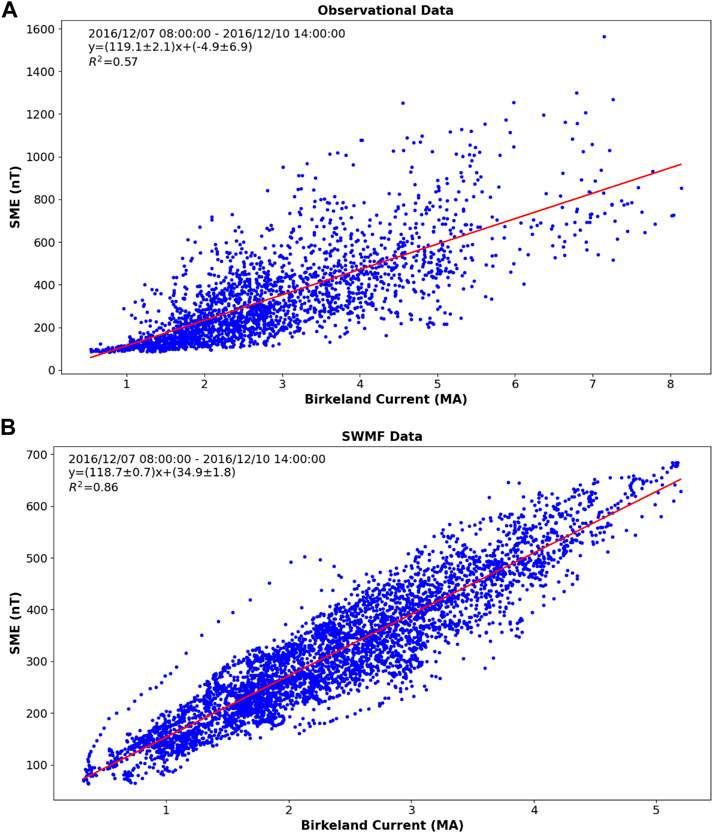
FIGURE 1. The relationship between SME and total Birkeland Current as determined by observations (A) and by SWMF (B) for a Winter event. The data points presented here are for 2 min intervals.

FIGURE 2

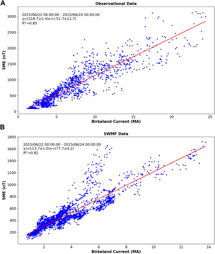
FIGURE 2. The relationship between SME and total Birkeland Current as determined by observations (A) and by SWMF (B) for a summer event.

FIGURE 3

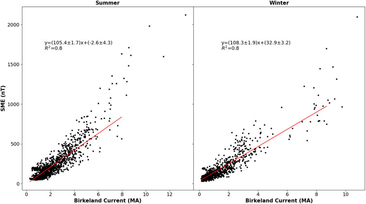
FIGURE 3. Figure from James and Lopez 2022. Observational data displaying the relationship between the auroral electrojet and field-aligned current for summer and Winter.

FIGURE 4

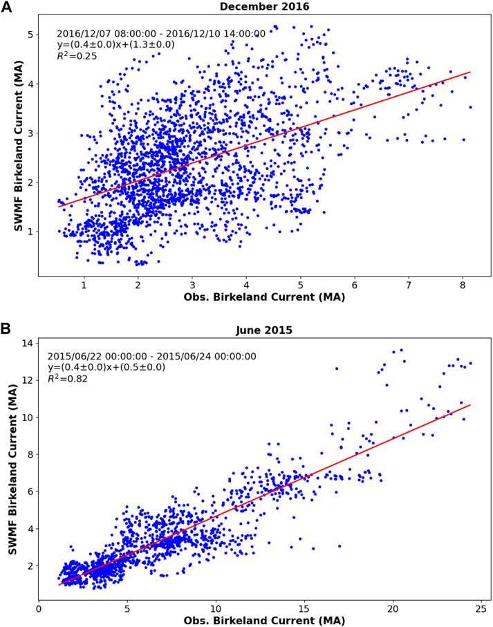
FIGURE 4. Observations and SWMF Birkeland current for Winter (A) and summer (B) Events. The currents for the summer event is more strongly correlated than those during the Winter event.

3.2 Seasonal ratio

To examine the seasonal asymmetry between currents we take a look at simulation results from four periods. These periods are: 2011 December 18–25, 2016 December 7–10, 2011 June 18–25, and 2015 June 22–24, days 18–25 of each month. The June 2015 period was driven with data from ACE, the December 1026 period was driven with data from Wind, and the other two periods were driven using the OMNI dataset. For December 2011, the magnitude of the currents in the Southern Hemisphere are larger than the currents in the Northern hemisphere (Figure 5). For June 2011 and June 2015, the currents are larger in the Northern Hemisphere (Figures 6, 7). These periods reproduce the expected seasonal asymmetry with the sunlit polar region having larger currents. However, for the December 2016 period the simulated currents are larger in the Northern Hemisphere compared to the Southern Hemisphere (Figure 8). We would expect the opposite behavior, if we only consider the conductivity resulting from the seasonal asymmetry in solar irradiation.

FIGURE 5

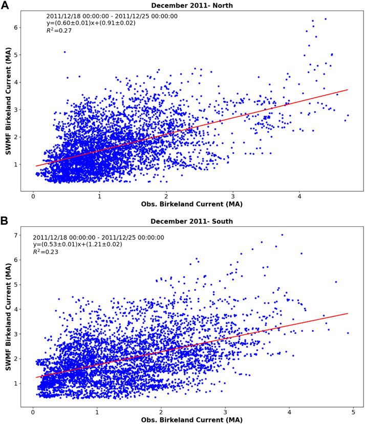
FIGURE 5. Observations and SWMF Birkeland current for December 2011. (A) Northern Hemisphere (B) Southern Hemisphere.

FIGURE 6

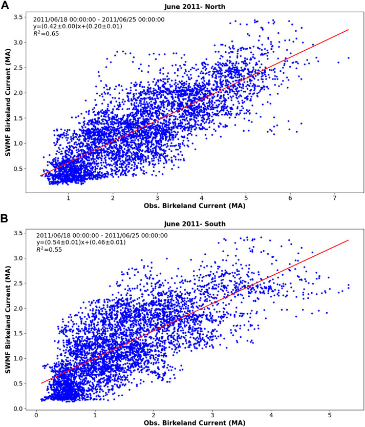
FIGURE 6. Observations and SWMF Birkeland current for June 2011. (A) Northern Hemisphere (B) Southern Hemisphere.

FIGURE 7

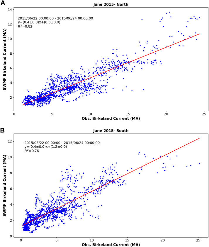
FIGURE 7. Observations and SWMF Birkeland current for June 2015. (A) Northern Hemisphere (B) Southern Hemisphere.

FIGURE 8

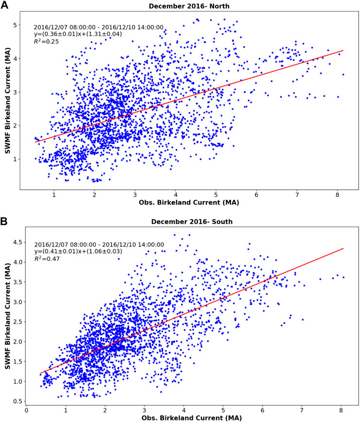
FIGURE 8. Observations and SWMF Birkeland current for December 2016. (A) Northern Hemisphere (B) Southern Hemisphere.

Examining the entire period, the average total simulated Birkeland current was 2.36 MA in the Northern Hemisphere and 2.15 MA in the Southern Hemisphere. The AMPERE data had an average total Birkeland current of 2.93 MA in the Northern Hemisphere and 2.68 MA in the Southern Hemisphere. There are two items to note in this comparison. First the interhemispheric asymmetry is the same in both the observations and the simulation. Second, the pattern of the simulated currents being less than the observed current shows up in the averages. The fact that both the observations and the simulations have an asymmetry opposite to that expected from the asymmetry in the F10.7 flux suggests that this is a real effect. At present, we do not have an explanation for this finding, however, inspecting the AMPERE dataset, we find many examples in winter months of the total Birkeland current in the Northern (dark) Hemisphere being larger than the current in the Southern (sunlit) Hemisphere. On the other hand, we do not find the reverse; it is quite rare is the summer months for the Southern (dark) Hemisphere to have larger total Birkeland current than the current in the Northern (sunlit) Hemisphere. This finding requires significant investigation beyond the scope of this paper to quantify and explain.

For all the events the correlation coefficients between the observed and simulated currents are poor and is indicative of the difficulty of SWMF to replicate reality reliably. However, in the previous subsection, we have shown that SWMF’s inability to replicate the actual values and variations in the observed currents to have no bearing on how well the model is able to replicate the relationship between the simulated Birkeland current magnitude and simulated SME. In other words, the model is always showing the current closure relationship weather or not it gets the actual values of the currents corresponding to reality. Therefore, if you were making observations of FACs and running simulations and the magnitude of the total observed FAC is different from that simulated, you can be assured that the magnitude of the simulated SME will also not correlate to the magnitude of the observed SME. From these results, we can say the correlation coefficients are not necessarily an indicator of how well interhemispheric conductivity is being replicated.

3.3 F10.7 study

F10.7 is a proxy for the measure of solar irradiation. We expect as F10.7 increases there would also be an increase in the amount of current in the ionosphere. Additionally, we expect as F10.7 increases for the potential across the ionosphere to decrease, as a consequence of the change in geoeffective length (Lopez et al. (2010), consistent with observed F10.7 dependence of the position of the nose of the magnetopause (Němeček et al., 2016).

To examine this question, we consider a 1-week period centered on the winter solstice in December of 2010. For two different runs, we fixed the value of F10.7, then simulated the period using the SWMF driven by the original solar wind time series. One run had a fixed F10.7 of 80 and the other has an F10.7 of 180. We consider F10.7 of 80 to be a reference value for low solar EUV flux and F10.7 of 180 to be a reference high value. We find that as F10.7 increases, the ionospheric potential in both hemispheres decreases, as seen in Figures 9, 10. This is what is expected (Lopez et al., 2010), that higher conductivity results in a lower ionospheric potential.

FIGURE 9

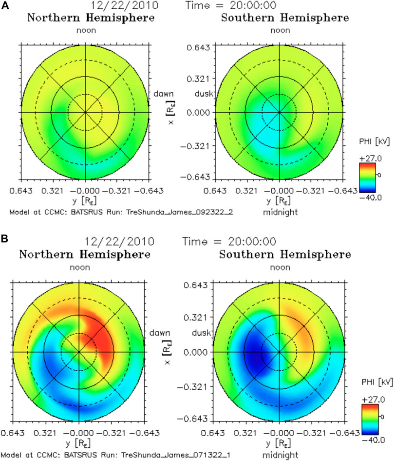
FIGURE 9. (A) Potential map for F10.7 of 180. (B) Potential map for F10.7 of 80.

FIGURE 10

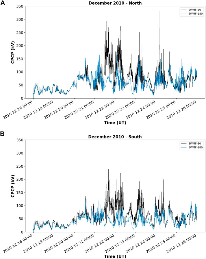
FIGURE 10. The time series for the SWMF calculated cross polar cap potentials (CPCP) for F10.7 of 80 (black) and 180 (blue). (A) Shows the CPCP in the Northern Hemisphere. (B) Displays the CPCP in the Southern Hemisphere.

In contrast to the simulation results for the potential, the average total Birkeland currents for the two runs do not show exactly the same pattern as determined from observations (James and Lopez, 2022). Table 1 presents the average Birkeland current for the two runs in the Northern and Southern Hemispheres. The expected seasonal asymmetry is present in both the low and high F10.7 runs, with the summer (southern) hemisphere having larger average current. However, both hemispheres had lower average Birkeland current values in the higher F10.7 runs (which also had the lower potentials). Observations show that on average the sunlit (summer) hemisphere has a larger Birkeland current for higher values of F10.7, while the dark (winter) hemisphere has smaller Birkeland current. This was interpreted as being due to the variation in conductance with solar radiation and the unequal amounts of solar EUV conductance in the two hemispheres (James and Lopez, 2022).

TABLE 1

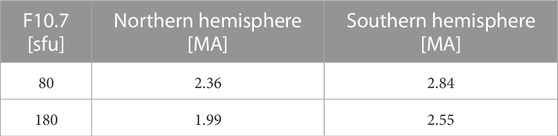
TABLE 1. Average Birkeland current magnitudes with varying F10.7 for SWMF simulation of 2010 December 18–25.

In MHD global models, the Knight Relation is used to get an estimate of electron flux (Knight, 1973) and an empirical relationship is used to calculate the Hall and Pedersen conductances due to precipitating particles (Robinson et al., 1987). This conductance is then added to the solar EUV conductance to determine the overall conductivity (Fedder et al., 1995). However, in Wiltberger et al. (2004), the authors conducted a direct comparison and found this traditional calculation of the conductivity to be insufficient, because the MHD model used consistently underestimated the electron precipitation and over-estimated the cross-polar cap potential (CPCP) as compared to observations. In SWMF, rather than using the Knight Relation for the conductivity, this model uses a different empirical relationship. The runs in this study use an empirical relation between the FAC and conductance based on AIMEE data (i.e., the Ridley Legacy Model). A detailed description of this model can be found in Mukhopadhyay et al., 2020.

It is possible that the EUV conductance model is not fully representative of the contribution to the total conductance and that it also contributes to the underestimation of the conductance, which leads to high potentials. Thus, a possible explanation for the fact that the SWMF reproduced the expected trend of the potential with F10.7, but not the observed trend in the total Birkeland current with F10.7 could be due to a need for a more realistic conductivity model. In fact, inspecting Figure 10, one can see that the values of the potential are high, often exceeding 150 KV in both hemispheres for the low F10.7 run. But such large potentials are only observed during geomagnetic storms and for the period simulated the solar wind was very moderate, with southward IMF barely exceeding 5 nT a handful of times and flow speed generally below 400 km/s. Therefore, it is clear that the simulation was producing unrealistically large ionospheric potentials due to an unrealistically low ionospheric conductivity.

4 Conclusion

We have conducted an investigation of the ability of the SWMF to replicate the observed SME index and the magnitude of the Birkeland currents as observed by AMPERE. We find that for some events, the correlation between the observed quantities and the simulated quantities are good. However, the simulated Birkeland currents and SME index are generally smaller than the observed quantities during these “good” events. On the other hand, the relationships between the simulated Birkeland current and the simulated SME is quite similar to the same relationship obtained from observations. This is consistent with the interpretation that this relationship is an expression of current closure, with the electrojets closing the Birkeland current system. Moreover, this relationship exists in the simulation data irrespective of the correlation between the simulations and observations for a given event, which also supports this interpretation.

The simulation however, does not always reproduce the seasonal asymmetry in the currents. Observations indicate that the currents are larger in the summer hemisphere, and sometimes this is what the SWMF simulations produce, but not always as can be seen in the December 2016 solstice week, the simulation gives the opposite result. The simulation result for December 2016 is mirrored in the AMPERE data; to understand this apparent anomaly in both simulation and observational results requires additional study. The simulation also replicates the expected variation in the ionospheric potential with F10.7, with larger F10.7 yielding lower ionospheric potentials. However, the simulation do not entirely replicate the behavior of the total Birkeland current seen in observations. We conclude that better models for the ionospheric conductance are required.

Data availability statement

The original contributions presented in the study are included in the article/Supplementary Material, further inquiries can be directed to the corresponding author.

Author contributions

TJ and RL contributed to conception and design of the study. TJ analyzed the MHD simulations. All authors contributed to the analysis of the events studied. TJ wrote the first draft of the manuscript. All authors contributed to the article and approved the submitted version.

Funding

We acknowledge the support of the US National Science Foundation (NSF) under Grant No. 1916604. We also acknowledge the support of The National Aeronautics and Space Administration (NASA) under Grant No. 80NSSC20K0606 [The Center for the Unified Study of Interhemispheric Asymmetries (CUSIA)] and Grant No. 80NSSC21K2057.

Acknowledgments

We gratefully acknowledge the SuperMAG website and the data there provided by SuperMAG collaborators (http://supermag.jhuapl.edu). We thank the AMPERE team and the AMPERE Science Center for providing the Iridium derived data products (http://ampere.jhuapl.edu). Simulation results have been provided by the Community Coordinated Modeling Center at Goddard Space Flight Center through their publicly available simulation services (https://ccmc.gsfc.nasa.gov). We acknowledge use of NASA/GSFC’s Space Physics Data Facility’s OMNIWeb (or CDAWeb or ftp) service, and OMNI data.

Conflict of interest

The authors declare that the research was conducted in the absence of any commercial or financial relationships that could be construed as a potential conflict of interest.

Publisher’s note

All claims expressed in this article are solely those of the authors and do not necessarily represent those of their affiliated organizations, or those of the publisher, the editors and the reviewers. Any product that may be evaluated in this article, or claim that may be made by its manufacturer, is not guaranteed or endorsed by the publisher.

References

Anderson, B. J., Takahashi, K., and Toth, B. A. (2000). Sensing global birkeland currents with iridium® engineering magnetometer data. Geophys. Res. Lett. 27, 4045–4048. doi:10.1029/2000GL000094

CrossRef Full Text | Google Scholar

De Zeeuw, D., Sazykin, S., Ridley, A., Toth, G., Gombosi, T., Powell, K., et al. (2001). Inner magnetosphere simulations-coupling the Michigan mhd model with the rice convection model. AGU Fall Meet. Abstr. 2001, SM42A–0830.

Google Scholar

Dungey, J. W. (1961). Interplanetary magnetic field and the auroral zones. Phys. Rev. Lett. 6, 47–48. doi:10.1103/physrevlett.6.47

CrossRef Full Text | Google Scholar

Fedder, J. A., Slinker, S. P., Lyon, J. G., and Elphinstone, R. (1995). Global numerical simulation of the growth phase and the expansion onset for a substorm observed by viking. J. Geophys. Res. Space Phys. 100, 19083–19093. doi:10.1029/95ja01524

CrossRef Full Text | Google Scholar

Fok, M.-C., Buzulukova, N. Y., Chen, S.-H., Glocer, A., Nagai, T., Valek, P., et al. (2014). The comprehensive inner magnetosphere-ionosphere model. J. Geophys. Res. Space Phys. 119, 7522–7540. doi:10.1002/2014JA020239

CrossRef Full Text | Google Scholar

Gjerloev, J. W. (2012). The supermag data processing technique. J. Geophys. Res. Space Phys. 117. doi:10.1029/2012JA017683

CrossRef Full Text | Google Scholar

Glocer, A., Rastätter, L., Kuznetsova, M., Pulkkinen, A., Singer, H., Balch, C., et al. (2016). Community-wide validation of geospace model local k-index predictions to support model transition to operations. Space weather. 14, 469–480. doi:10.1002/2016sw001387

CrossRef Full Text | Google Scholar

Gordeev, E., Sergeev, V., Honkonen, I., Kuznetsova, M., Rastätter, L., Palmroth, M., et al. (2015). Assessing the performance of community-available global mhd models using key system parameters and empirical relationships. Space weather. 13, 868–884. doi:10.1002/2015sw001307

CrossRef Full Text | Google Scholar

Honkonen, I., Rastätter, L., Grocott, A., Pulkkinen, A., Palmroth, M., Raeder, J., et al. (2013). On the performance of global magnetohydrodynamic models in the earth’s magnetosphere. Space weather. 11, 313–326. doi:10.1002/swe.20055

CrossRef Full Text | Google Scholar

James, T., and Lopez, R. E. (2022). The effect of f10. 7 on interhemispheric differences in ionospheric current during solstices. Adv. Space Res. 69, 2951–2956. doi:10.1016/j.asr.2022.02.006

CrossRef Full Text | Google Scholar

Janhunen, P., Palmroth, M., Laitinen, T., Honkonen, I., Juusola, L., Facskó, G., et al. (2012). The gumics-4 global mhd magnetosphere–ionosphere coupling simulation. J. Atmos. Solar-Terrestrial Phys. 80, 48–59. doi:10.1016/j.jastp.2012.03.006

CrossRef Full Text | Google Scholar

Knight, S. (1973). Parallel electric fields. Planet. Space Sci. 21, 741–750. doi:10.1016/0032-0633(73)90093-7

CrossRef Full Text | Google Scholar

Laundal, K. M., Cnossen, I., Milan, S. E., Haaland, S., Coxon, J., Pedatella, N., et al. (2017). North–south asymmetries in earth’s magnetic field. Space Sci. Rev. 206, 225–257. doi:10.1007/s11214-016-0273-0

CrossRef Full Text | Google Scholar

Lopez, R., Bruntz, R., Mitchell, E., Wiltberger, M., Lyon, J., and Merkin, V. (2010). Role of magnetosheath force balance in regulating the dayside reconnection potential. J. Geophys. Res. Space Phys. 115. doi:10.1029/2009ja014597

CrossRef Full Text | Google Scholar

Lyon, J., Fedder, J., and Mobarry, C. (2004). The lyon–fedder–mobarry (lfm) global mhd magnetospheric simulation code. J. Atmos. Solar-Terrestrial Phys. 66, 1333–1350. doi:10.1016/j.jastp.2004.03.020

CrossRef Full Text | Google Scholar

Mukhopadhyay, A. (2022). Statistical comparison of magnetopause distances and cpcp estimation by global mhd models. Authorea. Preprints. doi:10.1002/essoar.10502157.1

CrossRef Full Text | Google Scholar

Mukhopadhyay, A., Welling, D. T., Liemohn, M. W., Ridley, A. J., Chakraborty, S., and Anderson, B. J. (2020). Conductance model for extreme events: impact of auroral conductance on space weather forecasts. Space weather. 18, e2020SW002551. doi:10.1029/2020sw002551

CrossRef Full Text | Google Scholar

Němeček, Z., Šafránková, J., Lopez, R., Dušík, Š., Nouzák, L., Přech, L., et al. (2016). Solar cycle variations of magnetopause locations. Adv. Space Res. 58, 240–248. doi:10.1016/j.asr.2015.10.012

CrossRef Full Text | Google Scholar

Pulkkinen, A., Rastätter, L., Kuznetsova, M., Singer, H., Balch, C., Weimer, D., et al. (2013). Community-wide validation of geospace model ground magnetic field perturbation predictions to support model transition to operations. Space weather. 11, 369–385. doi:10.1002/swe.20056

CrossRef Full Text | Google Scholar

Raeder, J., Larson, D., Li, W., Kepko, E. L., and Fuller-Rowell, T. (2009). Openggcm simulations for the themis mission. THEMIS Mission 141, 535–555. doi:10.1007/s11214-008-9421-5

CrossRef Full Text | Google Scholar

Ridley, A., and Kihn, E. (2004). Polar cap index comparisons with amie cross polar cap potential, electric field, and polar cap area. Geophys. Res. Lett. 31. doi:10.1029/2003gl019113

CrossRef Full Text | Google Scholar

Ridley, A., and Liemohn, M. (2002). A model-derived storm time asymmetric ring current driven electric field description. J. Geophys. Res. Space Phys. 107, SMP 2-1–SMP 2-12. doi:10.1029/2001ja000051

CrossRef Full Text | Google Scholar

Robinson, R., Vondrak, R., Miller, K., Dabbs, T., and Hardy, D. (1987). On calculating ionospheric conductances from the flux and energy of precipitating electrons. J. Geophys. Res. Space Phys. 92, 2565–2569. doi:10.1029/ja092ia03p02565

CrossRef Full Text | Google Scholar

Toffoletto, F., Sazykin, S., Spiro, R., and Wolf, R. (2003). Inner magnetospheric modeling with the rice convection model. Space Sci. Rev. 107, 175–196. doi:10.1023/a:1025532008047

CrossRef Full Text | Google Scholar

Tóth, G., Sokolov, I. V., Gombosi, T. I., Chesney, D. R., Clauer, C. R., De Zeeuw, D. L., et al. (2005). Space weather modeling framework: A new tool for the space science community. J. Geophys. Res. Space Phys. 110, A12226. doi:10.1029/2005ja011126

CrossRef Full Text | Google Scholar

Waters, C. L., Anderson, B. J., and Liou, K. (2001). Estimation of global field aligned currents using the iridium® system magnetometer data. Geophys. Res. Lett. 28, 2165–2168. doi:10.1029/2000GL012725

CrossRef Full Text | Google Scholar

Wiltberger, M., Wang, W., Burns, A., Solomon, S., Lyon, J., and Goodrich, C. (2004). Initial results from the coupled magnetosphere ionosphere thermosphere model: magnetospheric and ionospheric responses. J. Atmos. Solar-Terrestrial Phys. 66, 1411–1423. doi:10.1016/j.jastp.2004.03.026

CrossRef Full Text | Google Scholar