Why can the auroral-type sporadic E layer be detected over the South America Magnetic Anomaly (SAMA) region? An investigation of a case study under the influence of the high-speed solar wind stream

The low-electron flux variability (increase/decrease) in the Earth’s radiation belts could cause low-energy Electron Precipitation (EP) to the atmosphere over auroral and South American Magnetic Anomaly (SAMA) regions. This EP into the atmosphere can cause an extra upper atmosphere’s ionization, forming the auroral-type sporadic E layers (Esa) over these regions. The dynamic mechanisms responsible for developing this Esa layer over the auroral region have been established in the literature since the 1960s. In contrast, there are several open questions over the SAMA region, principally due to the absence (or contamination) of the inner radiation belt and EP parameter measurements over this region. Generally, the Esa layer is detected under the influence of geomagnetic storms during the recovery phase, associated with solar wind structures, in which the time duration over the auroral region is considerably greater than the time duration over the SAMA region. The inner radiation belt’s dynamic is investigated during a High-speed Solar wind Stream (September 24-25, 2017), and the hiss wave-particle interactions are the main dynamic mechanism able to trigger the Esa layer’s generation outside the auroral oval. This result is compared with the dynamic mechanisms that can cause particle precipitation in the auroral region, showing that each region presents different physical mechanisms. Additionally, the difference between the time duration of the hiss wave activities and the Esa layers is discussed, highlighting other ingredients mandatory to generate the Esa layer in the SAMA region.

Highlights

• The low-energy electron injections (≤100 keV) between L* = 2.8 and 3.0 are observed during the conjunction between VAP-B and Santa Maria station.

• The level of low-energy electron precipitation (EP) predominant defines the base height of the Esa layer.

• The maximum peak of the ionization rate integrated defines the maximum critical frequency of the Esa layer.

1 Introduction

The generating mechanism of the auroral-type sporadic E (Esa) layers detected in the auroral oval has been well understood since the 1960s (Rees, 1963). In the auroral oval, low energy electron precipitation (EP) originating from the magnetosphere and Solar Energetic Particles (SEPs) are primarily responsible for producing auroral-type sporadic E. These mechanisms operate exclusively in the auroral regions (Whitehead, 1970). In addition, Esa layers can be generated in the low/middle-latitude, specifically over South America, due to the presence of the South American Magnetic Anomaly (SAMA) (Batista and Abdu, 1977; Moro et al., 2022a; Da Silva et al., 2022). Esa layers over South America have a different generating mechanism from those in the auroral zone, which is thought to be related to the geometric configuration of the geomagnetic field (Pinto and Gonzalez, 1989) that contributes to the inner boundary of the inner radiation belt being deeper compared to the other point of the same latitude around the globe (Roederer, 1967). These pronounced departures in geomagnetic field symmetry promote proton contamination in the electron measurements, as well as the low-energy electron precipitation over the SAMA region, which results in a significant impact on the local ionosphere, such as the generation of the auroral-type sporadic E layer, detected since the 1970s (Batista and Abdu, 1977). The electron energy range able to generate the Esa layers over the auroral oval is ≥1 keV (Rees, 1963; Cai and Ma, 2007), while over the SAMA region, it is between 0.5 keV and tens keV (see Da Silva et al., 2022). The dynamic mechanisms responsible for electron precipitation in both auroral ovals and the SAMA region are completely different (Da Silva et al., 2022). Therefore, they can generate different characteristics in these Esa layers when detected in these distinct regions, such as the time duration, intensity, position in altitude, as well as frequency range (Resende et al., 2022b).

The low-energy EP over the auroral oval can be originated in the outer radiation belt. They can occur through the wave-particle resonances driven by the whistler-mode chorus, plume, and magnetosonic waves. Generally, the low-energy EP over the auroral oval occurs during the geomagnetic storms and substorms under the influence of the different solar wind structures (Horne et al., 2009; Rodger et a., 2010; Meredith et al., 2011). The generator mechanisms of the Esa layer over the auroral oval regions are well known, principally due to the exclusive dependence on low-energy EP of this kind of sporadic E layer in these regions (Resende et al., 2022b).

Conversely, the main dynamic mechanism responsible for causing the low-energy EP over the SAMA region under the influence of an Interplanetary Coronal Mass Ejection (ICME) is the pitch angle scattering driven by hiss waves (Da Silva et al., 2022). Therefore, this low-energy EP can trigger the generator mechanisms of the Esa layer over this peculiar region during the recovery phase of the geomagnetic storm (Batista and Abdu, 1977; Moro et al., 2022a; Da Silva et al., 2022). On the other hand, the dynamic mechanism over the SAMA region able to trigger the generator mechanisms of the Esa layer under the influence of a High-Speed solar wind Stream (HSS) needs to be identified, including the role of the magnetospheric waves in the low-energy EP over this region. Thus, the inner radiation belt dynamic and its impact on the local ionosphere will be discussed to answer the question in the title of this paper, considering the influence of an HSS.

The low-energy EP is not a unique ingredient in developing the sporadic E layer over SAMA. The wind shear mechanism is fundamental to the Es layer development at low and middle latitudes. These Es layer occurrences are classified as blanketing (Esb) layers. In this process, the molecular and the metallic ions are converged in thin layers due to the tidal wind components. In fact, the zonal and meridional winds in opposite directions carry the ions, and due to the magnetic field, the Lorentz force causes a vertical movement of these ions. Thus, there is an accumulation of the ions in the null points of the tidal winds generating a dense thin ionization layer compared to the background (Chimonas and Axford 1968). Therefore, the upper atmospheric wind conditions are also important and must be considered (Rees, 1963; Cai and Ma, 2007; Resende et al., 2022b; Resende et al., 2022c).

2 Data set and methodology

A case study under the influence of an HSS was selected to analyze and to compare the physical processes related to the auroral-type sporadic E (Esa) layers detected over the low/middle-latitude and auroral regions. This comparison between the physical processes in the outer and inner radiation belt will answer the questions about this kind of sporadic E layer detected outside the auroral region. The satellite and ground-based data are employed to develop these analyses. The interplanetary medium conditions, the dynamic mechanisms, such as the wave-particle interaction in the radiation belts, and their impact on the ionosphere over the SAMA region will be discussed to be better understood.

The HSS’s characteristics are discussed from parameters measured by the Magnetic Field Experiment (MAG) and Solar Wind Electron, Proton, and Alpha Monitor (SWEPAM) onboard the Advanced Composition Explorer (ACE) satellite, which provides the solar wind parameters at the L1 Lagrangian point (Stone et al., 1998). The geomagnetic index (Auroral electrojet - AE) available at OMNIWeb (https://omniweb.gsfc.nasa.gov/) is used to describe the different substorm periods. The Esa layers are detected over the SAMA’s center using the ionosonde installed at Santa Maria (29.7°S, 53.8°W, dip (I): ∼-37°, L: 1.16). The ionosonde measurements at Tromso (69.7°N, 18°E, dip (I): ∼78°, L: 6.45) will be used only for the comparison with the SAMA’s results. The dip, or geomagnetic inclination (I), is the angle between the horizontal plane and the total field vector (e.g., Chulliat et al., 2020).

The low-energy EP over the SAMA’s center and auroral oval regions are discussed using the measurements in situ (radiation belts) of the low-energy electron injections from the Magnetic Electron Ion Spectrometer (MagEIS) instrument (Blake et al., 2013), and Helium, Oxygen, Proton, and Electron (HOPE) instrument (Funsten et al., 2013) onboard Van Allen Probe B (Mauk et al., 2013). The MagEIS data has been reprocessed by Claudepierre et al. (2015) to correct for proton contamination close to perigee. The SAMA region is significantly contaminated by protons, and it is impossible to use the available low-orbit satellite data to measure low-energy EP directly. The low-energy electron injections are also analyzed through the time evolution of phase space density (PhSD [c/(cm MeV))³ sr⁻¹]), which PSD data was obtained from MagEIS instrument onboard Van Allen Probe B available at https://rbspgway.jhuapl.edu/psd.

The whistler mode chorus waves outside the plasmapause (hundreds of Hz up to about 10 kHz) (Gurnett and O'Brien, 1964), plume whistler mode waves in plasmaspheric plumes (Su et al., 2018; Li et al., 2019), and whistler mode hiss waves inside the plasmasphere (20 Hz to a few kHz) (Meredith et al., 2004) are analyzed. The whistler waves are plasma waves, right circularly polarized, observed in the magnetosphere (Helliwell, 1965), in which can interact resonantly with the low-energy electron to launch these particles to the loss cone, followed by the precipitation into the atmosphere in the auroral oval and SAMA regions (Horne et al., 2009; Rodger et al., 2010; Li et al., 2019; Da Silva et al., 2022). Therefore, the power spectral densities of the magnetic field and total electron density are used to detect these whistler mode waves and the plasmapause position (Lpp), respectively. The polarization properties, such as the wave Normal Angle (WNA), ellipticity, and planarity, are calculated through the singular value decomposition method (Santolík et al., 2003). These parameters are obtained from the Electric and Magnetic Field Instrument Suite and Integrated Science (EMFISIS) (Kletzing et al., 2013) onboard Van Allen Probes (Mauk et al., 2012).

3 Interplanetary medium parameters during the influence of a HSS

The solar wind parameters, interplanetary magnetic field (IMF), and AE index are presented in Figure 1. The interplanetary medium conditions are here described, emphasizing the substorms duration associated with an HSS that reached L1 Lagrangian point on 24 September 2017. Panel (a) and (b) shows the solar wind velocity (Vp) and proton density (particles/cm-3), respectively, in which solar wind velocity reached the maximum value (420 km s⁻¹) close to 04:00 UT and 08:30 UT, respectively, on September 25. The proton density reached values above 30 particles/cm⁻³, followed by a decrease in a few hours. The maximum proton density value is almost concurrent with the negative Bz component of the IMF (panel d - red line). Bx (panel c - red line) and By (panel c - blue line) components of the IMF are not so strong and remain preferentially positive and negative, respectively, in which the Alfvenic fluctuations are observed in Vx component during some periods as shown in Supplementary Figure S1 (Supporting Information). The concept of Alfvénicity in the context of solar wind refers to the degree to which the solar wind plasma and magnetic field exhibit characteristics associated with Alfvén waves. The Alfvénic fluctuations of the IMF are commonly observed during the long recovery phases of the HSS (Da Silva et al., 2019; Da Silva et al., 2021b). This behavior in IMF, generally is observed simultaneously with moderate substorms activities, followed by intermittent intervals of enhanced magnetospheric convection that contribute to the low-energy electron injections into the radiation belts (e.g., Forsyth et al., 2016).

FIGURE 1

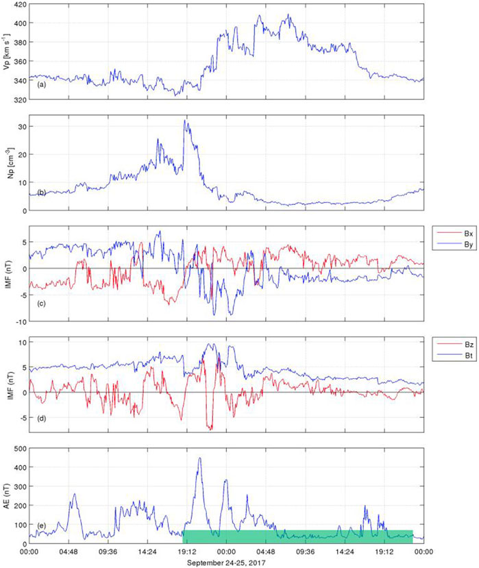
FIGURE 1. (A) Solar wind velocity (Vp); (B) Proton density (Np); (C) Bx component and By component of the Interplanetary Magnetic Field (IMF); (D) B total (Bt) and Bz component of the IMF; and (E) Auroral electrojet (AE) index. The IMF components are in GSM coordinates. The green box is referent to the period of analysis. The HSS reached L1 Lagrangian point on 24 September 2017.

The auroral electrojet (AE) index (panel e) reached the maximum value close to 450 nT almost simultaneously with the strong value of the proton density. The subsequent AE index peaks are not strong, reaching values from 75 nT to 345 nT. It means that the substorms associated with this HSS are considerably weak. It suggests that the low-energy electron injections in the inner magnetosphere under the influence of these substorms may also be weak both in flux intensity and in-depth that the particles reach in the radiation belts, compared to the low-energy electron injections in the inner magnetosphere under the influence of ICMEs (e.g., Da Silva et al., 2022). In subsequent sections, this behavior will be discussed to highlight the different physical processes at the L1 Lagrangian point and their impact on the inner magnetosphere and ionosphere.

4 Auroral-type sporadic E layer detected over the SAMA region

The ionograms from the Digisonde located at Santa Maria station detected the auroral-type sporadic E layer (Esa) over the SAMA region only during two periods (06:00 UT—07:00 UT and 22:05 UT—22:25 UT on 25 September 2017, in which are under the influence of the HSS that reached at L1 Lagrangian point on 24 September 2017. Figures 2A, B shows the Esa layers detected during the first and second periods, which are indicated through the red arrows. Curiously, these Esa Layers detected over the SAMA region are generated under the influence of Alfvenic fluctuations in the Vx component, as shown in Supplementary Figure S1 (Supporting Information), which illustrates the linear correlation coefficients between Solar wind and Alfvén velocities. A high correlation coefficient can be associated to an Alfvenic nature of the solar wind, in which this observation is particularly evident in the top and bottom panels of the first row in Supplementary Figure S1, showing a high correlation between the fluctuations in the x component indicating a high Alfvenic solar wind (e.g., Da Silva et al., 2019; Da Silva et al., 2021b). The Esa Layers detected over the SAMA region under the influence of ICMEs were not previously observed concurrent with Alfvenic fluctuations but simultaneously with the recovery phase of the storm (see Batista and Abdu, 1977; Moro et al., 2022a; Da Silva et al., 2022). As discussed in the following sections, these different behaviors at L1 Lagrangian point trigger different physical processes in the magnetosphere and, consequently, in the ionosphere.

FIGURE 2

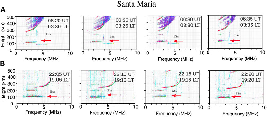
FIGURE 2. Ionograms from Digisonde located at Santa Maria station, which detected Esa layers only during the periods between 06:20 UT - 06:35 UT (03:30-03:35 LT, panel (A), and 22:05 UT - 22:20 UT (19:05 LT - 19:20 LT panel (B) on September, 25. The red arrows indicate the presence of the Esa layers. The color code in these ionograms represents the echo direction of the received signal. The thin “trace” at approximately 80 km is a technical artifact resulting from an error in the Digisonde processor.

Two types of Es layers over Santa Maria are observed, the Esa layer, formed due to particle precipitation, and the blanketing (Esb) layer, formed by wind shear. In fact, as Santa Maria is a transition region between the low and middle latitudes, the winds have high amplitudes, forming the Esb layers (Moro et al., 2022b). Generally, these winds are driven by the diurnal, semidiurnal, and terdiurnal tides present in the E region. Unfortunately, Santa Maria has no wind measurements during this related event. However, Andrioli et al. (2009) studied the mean winds and tides over Santa Maria from 2005 to 2007, and they showed a dominance of the diurnal tide in September with a maximum occurrence around 6:00 UT (zonal) and 12:00 UT (meridional) at around 100 km. Thus, the wind shear significantly influences the Es layer development over Santa Maria.

The competition between the particle precipitation and wind shear is seen mainly in panel (b) of Figure 2. It is noticed that the beginning of the F region trace is higher than 3 MHz. This behavior means that the Es layer blocked the F region in these hours, proving the action of the winds. Additionally, the maximum frequency in the cases of Figure 2B reached high values (more than 5 MHz, shown in red arrows). On the other hand, this fact was not observed in panel (a) of Figure 2, which is indicative that the particle precipitation was the principal mechanism of the Es layer formation at hours around 06:00 UT.

The ionograms from Digisonde located at Tromso station are presented and compared with the ionograms from Santa Maria station. The Tromso station detected Esa layers almost the entire period of the HSS influence, except close 06:00 UT on 25 September 2017. Supplementary Figure S2 (Supporting Information) shows the Esa layer detected between 21:00–23:30 UT on 24 September 2017 (panel a), and 22:00–22:45 UT on 25 September 2017 (panel b). The explanation of the absence of the Esa layer close 06:00 UT is directly related to the lack of plasma waves in the outer radiation belt at this period, which will be observed in Section 6. The Esa layers have a spreading trace over Tromso, as observed in Santa Maria. This behavior was discussed in Resende et al. (2022c), in which the pitch angle scattering driven by whistler mode chorus waves can cause low-energy EP (Da Silva et al., 2021a) over the auroral region. It is important to emphasize that the low-energy EP is a unique ingredient for developing the Esa layer over the auroral region. In contrast, the pitch angle scattering driven by plasmaspheric hiss waves (in the inner radiation belt) contributes to the particle precipitation over the SAMA (Da Silva et al., 2022), and there is a competition between the EP and the winds during the formation of the Esa layer over this region, which is observed in Figure 2B.

5 Conjunction between the Van Allen Probes and the ionosonde station over the SAMA’s center

The mechanisms responsible for the low-energy EP over auroral regions are widely studied, and the literature is well established (Rees, 1963; Whitehead, 1970), which means the generator mechanism of the Esa layer over this region is also well understood. The low-energy EP originated in the outer radiation belt can be analyzed here to discuss one crucial kind of physical process responsible for causing the EP over the auroral region, so it is not necessary to do the conjunction with the auroral region in the study because the behavior observed over Tromso station is similar to the other areas in the auroral oval. Another point is the measurements from the VAP-AB in the outer radiation belt are for a long time (apogee orbit). In contrast, the measurements in the inner radiation belt are brief (perigee orbit), in which the main analyses here will be concentrated in detail to explain the dynamic mechanisms responsible for causing the low-energy EP over the SAMA region.

These dynamic mechanisms within the inner radiation belt can cause electron particle precipitation over the SAMA region. They can trigger the physical processes responsible for generating the auroral-type sporadic E layer in this low-latitude (Da Silva et al., 2022). Thereby, using the Van Allen Probes data during their perigee orbit, it is possible to study the inner radiation belt conditions and their impact in the atmosphere for low L-shells (Da Silva et al., 2022) around the Earth. The interest here is in low L-shells over the SAMA region, which is necessary to find the conjunctions between the Van Allen Probes and Santa Maria station during the Esa layers detected on 25 September 2017.

Figure 3 shows the magnetic equator (red line) at 150 km of altitude, Van Allen probes orbit (blue line), and their footprint (blue dashed line) on 25 September 2017. The conjunctions can be observed when the blue dashed line crosses the Santa Maria station (red triangle), which is installed in the central region of the SAMA (white iso-intensity lines with 23,000 nT). Panel (a) shows the VAP-B orbit (6:00–6:30 UT) and panel (b) presents the VAP-A orbit (21:30–22:30 UT), periods of the Esa layers’ detection over SAMA. The conjunction between VAP-B and Santa Maria station (red triangle) was observed at 06:22 UT on 25 September 2017, in which the Magnetic Local Time (MLT) from VAP-B (MLT = 2.298) and Santa Maria station (MLT = 2.326) were almost coincident. The L values for both VAP-B and Santa Maria station were also almost coincident, presenting L = 1.23 and L = 1.16, respectively. On the other hand, the second period analyzed during this HSS observed a coincidence between VAP-A and Santa Maria station at 22:05 UT only in MLT, in which both show MLT = 18.029 and 18.032, respectively.

FIGURE 3

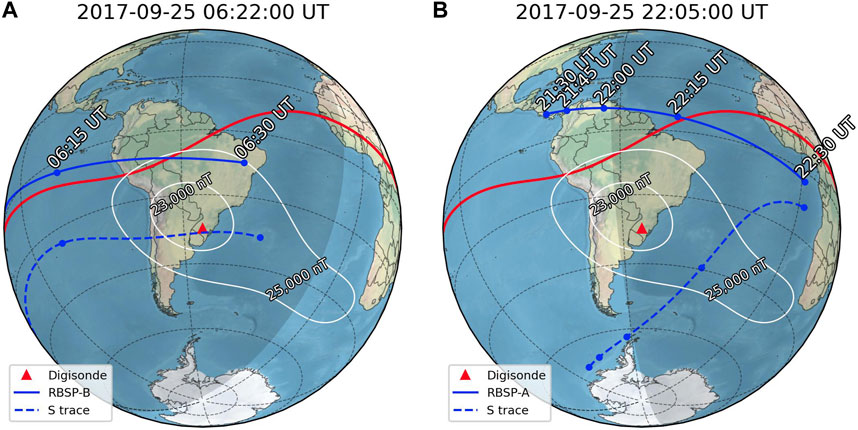
FIGURE 3. Magnetic equator (red line) at 150 km altitude, Van Allen probes orbit (blue line) and their footprint (blue dashed line) on 25 September 2017, for the two periods of the Esa layers detected. Panel (A) 06:22 UT and Panel (B) 22:05 UT. Santa Maria stations (red triangle) and the central region of the SAMA (white iso-intensity lines with 23,000 nT).

The discussions regarding the dynamic mechanisms inside the radiation belts will use only the data from the VAP-B due to the non-perfect conjunction using VAP-A and the proton contamination of the MagEIS instrument onboard VAP-A at the perigee.

6 Low-energy electron injections/precipitations and whistler mode wave activities within the radiation belts

The flux injections in this paper means the flux enhancements in different energy ranges (e.g., Sarris et al., 1976; Gabrielse et al., 2014) into the inner radiation belt (L-shell <2), which has been observed since 1990 decade, e.g., in Vampola and Korth, (1992), Baker et al. (1994), Xiao et al. (2009), and Shi et al. (2016), based on CRESS, SAMPEX, POLAR, and Van Allen Probes data mission, respectively. Cosmic Ray Albedo Neutron Decay (CRAND) is an important process to produce electrons locally in the inner radiation belt region during quiet geomagnetic periods (see Xiang et al., 2019; Li et al., 2023), although the decay rate of neutrons is considered relatively constant, in which could not explain the fast variability of the low-energy electrons flux in the inner radiation belt during the perturbed geomagnetic periods. High-energy electrons injections, i.e., > 100 keV are due to radial transport (see Li et al., 2023 and references therein) and magnetotail dipolarizations under substorms (Kim et al., 2021). The inner belt low energy electrons (<100 keV) dynamics can also follow processes similar to the higher energy populations. The enhancements of low energy electrons are observed more often (Reeves et al., 2015) and it can be related to fast magnetosonic wave interacting (Turner et al., 2015) under geomagnetic storms (Zhang et al., 2021).

Therefore, the main physical processes to explain the electrons flux injections in the inner radiation belt during the perturbed geomagnetic periods are interactions of the electrons with the fast magnetosonic waves, specifically in the Pi2 frequency range inside the plasmasphere (e.g., Zhao et al., 2014; Turner et al., 2015; Zhang et al., 2021; Li et al., 2023). The Pi2 cavity mode waves can explain the sudden enhancements of low-energy electrons at low L shells because this mode presents the electric field as an antinode within the plasmasphere, as discussed by Takahashi et al. (2003), in which the azimuthal electric field oscillation can interact resonantly with drifting energetic electrons, violating the third adiabatic invariant, and resulting in acceleration and radial injections crossing magnetic field lines (conserving the first and second adiabatic invariants) (e.g., Li et al., 1998; Turner et al., 2015).

On the other hand, three types of waves can scatter in low-energy electron resulting in loss of inner radiation belt electrons through resonance interactions (Li et al., 2015; Green et al., 2020; Hua et al., 2020; Li et al., 2023). Green et al. (2020) suggests that the lightning-generated whistlers (2–12 kHz) are important for scattering electrons from several hundred keV to several MeV at L ∼1.5. VLF transmitter waves play an important role in electron loss (e.g., Wang et al., 2018). The plasmaspheric hiss waves (∼50−10 kHz) can be responsible for the electron precipitation at the outer plasmasphere of tens to hundreds keV, as observed by Reeves et al. (2016), and below tens keV, as observed by Khazanov and Ma (2021). Therefore, the hiss waves are analyzed in this work due the interest in the scattering in energy level below 10 keV.

Figure 4 shows the low-energy electron injections for the energy channels of 75 keV and 169 keV (top panel) and the power spectral density (PSD) of the magnetic field (bottom panel) obtained from MagEIS and EMFISIS instruments, respectively, onboard Van Allen Probe B. Red, yellow and black lines represent 0.9 fce, 0.5 fce, 0.1 fce, in which fce is electron cyclotron frequency. The total electron density (medium panel) is used to identify the plasmapause position (Lpp). Plasmapause is a boundary between the low-density and high-density plasma regions, represented by the ratio variation between the maximum and minimum electron density (e.g., Lemaire, 1975; Thomas et al., 2021). Their position is essential to confirm the plasmaspheric wave activities.

FIGURE 4

FIGURE 4. (top panel) the low-energy electron flux (energy channels: 75 and 169 keV) obtained from MagEIS instrument. (medium panel) the total electron density obtained from the EMFISIS instrument. (bottom panel) the power spectral density of the magnetic field obtained from the EMFISIS instrument, in which the red, yellow and black lines represent 0.9 fce, 0.5 fce and 0.1 fce. Blue box is referent to the conjunction period between VAP-B and Santa Maria station. MagEIS and EMFISIS instruments are onboard the Van Allen Probe B.

The whistler mode chorus, plume, and plasmaspheric hiss waves are observed in Figure 4 (bottom panel) for almost the entire substorms period. The hiss waves are detected at all perigees, in which the low power (∼10⁻⁸ nT²/Hz) is observed only during the first perigee. The polarization properties, such as the wave Normal Angle (WNA), ellipticity, and planarity, are presented in Figure 5. They are calculated through the singular value decomposition method (Santolík et al., 2003) to confirm the presence of the hiss waves inside the plasmasphere (e.g., Li et al., 2015; 2019). WNA ≤40° (Figure 5 - top panel), ellipticity ≥0.5 (Figure 5 - medium panel), and planarity close to 0.5 (Figure 5 - bottom panel) are observed between 6:45-8:50 UT on September 2017, which are the same values observed by Li et al. (2015) and Da Silva et al. (2022) during the detection of the hiss waves.

FIGURE 5

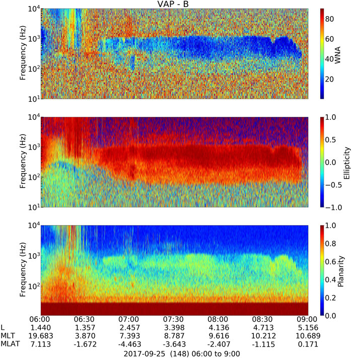
FIGURE 5. (top panel) Wave Normal Angle, (medium panel) ellipticity, and (bottom panel) Planarity are obtained from the EMFISIS instrument onboard Van Allen probe B at 6:00-9:00 UT on September 2017 (blue box period in Figure 4). These parameters are calculated through the singular value decomposition method (Santolík et al., 2003).

The low-energy electron injections (Figures 4 top panel) are observed during all periods of analyzed along all L-shells and are considerably more intense at the first 9 hours, which coincides with the first AE index peaks (Figure 1E). The low-energy electron injection peaks at high L-shells are concurrent with the whistler mode chorus and plume waves (bottom panel), suggesting the possible wave-particle interactions inside the outer radiation belt that may cause the low-energy EP to the atmosphere of the auroral regions.

The low-energy electron injection peaks (Figure 4 top panel) between 06:15 UT and 08:30 UT (blue box) are observed with more detail in Supplementary Figure S9. The concomitance between the power of whistler mode hiss waves of ∼10⁻⁵ nT²/Hz (Figure 4 - bottom panel) and electron injection peaks is observed from 6:57 UT in Supplementary Figure S8. These results are similar to those observed by Moro et al. (2022a) and Da Silva et al. (2022) during the low-energy electron precipitation over the SAMA region that contributed to the generator mechanism of the Esa layers. Although the presence of the hiss waves power of ∼10⁻⁵ nT²/Hz is evident from 6:57 UT (L-shell = 2.47), values of the hiss power below 10⁻⁵ nT²/Hz are observed inside the inner radiation belt (L-shell <2). Over the SAMA region, the power spectral density values of ∼10⁻⁵ nT²/Hz are also observed just above 500 Hz.

The electron injections over the SAMA region are observed close to 6:30 UT for the energy levels 75 keV and 350 keV in Supplementary Figure S9 and energy levels <10 keV in Supplementary Figure S10. It is essential to highlight that 6:30 UT is a time during the passage of the Van Allen Probe B over the SAMA region. The electron injection peaks <0.5 keV are also observed in Supplementary Figure S10, almost simultaneously with the Esa layer detected in Santa Maria station. This behavior observed in the electron flux injections within the inner radiation belt over the SAMA region concomitant with hiss wave activities suggests the possible wave-particle interactions that may cause the low-energy EP to the atmosphere of this region.

Although the whistler-mode hiss waves power of ∼10⁻⁵ nT²/Hz is similar during the influence of this HSS and the ICMEs (Moro et al., 2022a; Da Silva et al., 2022), the generator mechanisms of the hiss waves inside the inner radiation belt are completely different for each solar wind structure. For example, the plasmapause position generally is compressed during the recovery phase of the storms associated with the ICMEs and relaxed under the influence of the HSSs, which directly impacts the time duration and position of this kind of wave activity. Consequently, it can cause different impacts on the behavior of electron precipitation in the atmosphere.

Using the time evolution of the radial Phase Space Density (PhSD) profiles at inbound/outbound regions of the Van Allen Probe B it is possible to identify the electron injections energy levels and local (L*) of the injections. Therefore, the PhSD as a function of L*, calculated using a magnetic field model (TS04) (Tsyganenko & Sitnov, 2005), at fixed first (μ = 10 MeV/G) and second (K = 0.11 G1/2RE) adiabatic invariants (e.g., Hartley and Denton, 2014; Da Silva et al., 2019; Da Silva et al., 2021a) are presented in Figure 6. The PhSD profiles confirm the low-energy electron injections (∼100 keV) between L* = 2.8 and 3.0 (close to the inner radiation belt) during the conjunction between VAP-B and Santa Maria station, which was also observed in the blue box of Figure 4. It suggests the occurrence of the low-energy EP close to the SAMA region.

FIGURE 6

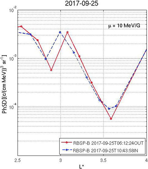
FIGURE 6. The Phase Space Density (PhSD) as a function of L* at μ = 10 MeV/G and K = 0.11 G^1/2R_E during the conjunction between VAP-B and Santa Maria station. PSD data was obtained from MagEIS instrument onboard Van Allen Probe B available in https://rbspgway.jhuapl.edu/psd.

The electron resonant kinetic energy is calculated using the dispersion relation presented in Eq. 1 (see Helliwell, 1965; Bittencourt, 1995; Alves et al., 2023) without the Lorentz factor.

$\omega -\overrightarrow{k}.\overrightarrow{v_e}=n{\mathrm{\Omega }}_{ce}(1)$

Where:

$\overrightarrow{k}$ is the wave number vector

ω is the frequency

$\overrightarrow{v_e}$ is the electron velocity vector

${\mathrm{\Omega }}_{ce}$ is the electron gyrofrequency

The gyrofrequency low-order harmonics $n=\pm 1,2,3\dots$

The range of electron kinetic energy able to resonantly interact with hiss waves is calculated using PSD of hiss waves in the time interval shown in the blue box (Figure 4), specifically at 08:00 UT on September 25. The second harmonic number is considered in the calculation, besides the ambient magnetic field at 379 nT and the electron density of 470 cm⁻³. In the selected time instant, the hiss emission occurred in broadband from 190 to 540 Hz (Supplementary Figure S3 - Supporting Information), leading to a resonant kinetic energy of ∼150 keV–60 keV, as shown in the gray area in Figure 7.

FIGURE 7

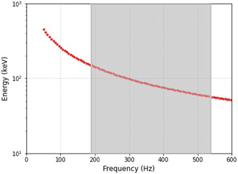
FIGURE 7. Resonant kinetic energy (in keV) for electrons as a function of hiss wave frequency propagating in a high-density plasmasphere. The gray vertical lines corresponds to the hiss wave frequency (in Hz) interval band observed in the plasmasphere at 08:00 UT on September 25 (shown in Figure 4; Supplementary Figure S3).

Although most studies regarding the interaction between hiss and electrons have shown strong efficiency in scattering electrons of 10 keV - 1 MeV energies, recently, studies presented by Khazanov and Ma (2021) have shown that the hiss waves can scatter electrons of energies below 10 keV down to tens of eV, which are coincident with the main energy range of interest in this work.

7 Atmospheric ionization over the SAMA and auroral oval regions (100–200 km)

The ionization rate altitude profiles over the SAMA region are calculated using an empirical model, which considers the isotropically precipitating electrons (100 eV–1 MeV) (Fang et al., 2010). The computed atmospheric ionization assumes that the incident particles (differential number flux, cm⁻² s⁻¹ keV⁻¹) have a Maxwellian distribution (e.g., Da Silva et al., 2022). The atmospheric ionization model (Fang et al., 2010) also can estimate the critical ionospheric frequency (MHz) altitude profile, which may be associated with the peak electron concentration [$N_e$ (electrons/m³)] of the Es layer by the relation $F_c=c\sqrt{N_e}$, where c = 8.98 (e.g., Nikolaeva et al., 2021; Da Silva et al., 2022).

The atmospheric ionization is calculated assuming that the incident particles, given by the differential number flux (cm^-2 s^-1 keV^-1) have a Maxwellian distribution, as defined by the function:

${\mathrm{\Phi }}_{\mathrm{M}}\left(\mathrm{E}\right)=\frac{{\mathrm{Q}}_0}{{2\mathrm{E}}_0^3}\text{Eexp}\left(-\frac{\mathrm{E}}{{\mathrm{E}}_0}\right),(2)$

Where the free parameters are:

${\mathrm{Q}}_0$ is the total energy flux in keV cm^-2 s^-1

${\mathrm{E}}_0$ is the characteristic energy in keV

${\mathrm{\Phi }}_{\mathrm{M}}$ is the differential number flux in cm^-2 s^-1 keV^-1

To estimate the incident energies and the atmospheric conditions is necessary to consider the variation of the days of the year and location, in which the geographic location (latitude and longitude), geomagnetic indices (F10.7 and Ap) and height scale (Supplementary Figure S4) are included in the model.

Initially, the total incident energy of electrons between 100 eV and hundreds of keV and the height scale (km) is estimated for Santa Maria station at 6:20 UT (first conjunction) and 22:05 UT (second conjunction) on 25 September 2017, as presented Figure 8; Supplementary Figure S6 (top panel - Supporting Information), respectively. The total incident energy of electrons during the second conjunction (Figure 8 red line) is slightly higher than the values during the first conjunction (Figures 8 blue line), which can cause influence the formation mechanisms of the Esa layer close to 100 km of altitude.

FIGURE 8

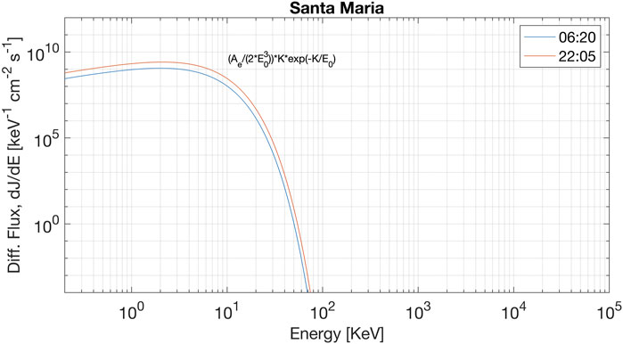
FIGURE 8. Total incident energy of electrons between 100 eV and hundreds of keV for Santa Maria station during the first (6:20 UT—blue line) and second (22:05 UT—red line) conjunction on 25 September 2017.

Figure 9 shows the total ionization rate altitude profiles (panels a and d), ionization rate altitude integrated (panels b and e), and critical ionospheric frequency (MHz) altitude, named here as frequency range altitude (panels c and f) for Santa Maria station during the first (6:20 UT—blue line) and second (22:05 UT—red line) conjunctions. The total ionization rate altitude profiles (panels a and d) presented significant values of the low-energy electrons (0.5 keV–10 keV) between 100 km–200 km of altitude for both analysis times. The previous sections suggested that the hiss waves have caused the precipitation of low-energy electrons to the atmosphere over the SAMA region through the pitch angle scattering mechanism (Li et al., 2019; Khazanov and Ma, 2021; Da Silva et al., 2022). However, the total ionization rate (panels a and d) and integrated (panels b and e) at the second conjunction is slightly more significant than the ionization rate at the first conjunction. This result caused a direct impact on frequency range altitude (panels c and f), in which the values above 3 MHz were reached during the first conjunction (panel c) and above 5 MHz during the second conjunction (panel f), which can trigger different generator mechanisms of the Esa layer in these periods.

FIGURE 9

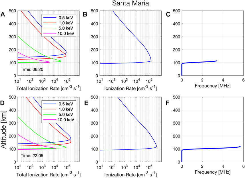
FIGURE 9. Ionization rate altitude profiles panels (A,D); ionization rate altitude integrated panels (B,E); and frequency range altitude for Santa Maria station panels (C,F). The time analyzed refers to the period of the conjunctions between VAP-AB and Santa Maria station.

The different values of the ionization rate during these conjunctions were expected due to the behavior of the total incident energy of the electron presented in Figure 8. On the other hand, the range of the low-energy electrons observed between 100 km–200 km of altitude is far above the results presented in Da Silva et al. (2022) for the same ionosonde station, principally due to the low/absence values of the 5 keV and the absence of the 10 keV, which contributed to the displacement of the Esa layer reaching values close to 150 km of altitude. Therefore, the level of low-energy electron precipitation (EP) predominant defines the base height of the Esa layer.

The critical modeled frequencies at 6:20 UT and 22:05 UT are included in the ionograms (Figure 10), and the relationship between the critical modeled frequencies and the maximum frequency reached by the Esa layer can be observed. The Esa layer at 22:05 UT reached a frequency greater than at 6:20 UT (Figure 11 first panels). It suggests a direct relationship exists between the ionization rate altitude profiles and the characteristics of the Esa layer. The electron energy levels ≥5 keV contributed to defining the Esa layer base height close to 100 km of altitude at 22:05 UT and 6:20 UT (Figures 10A, B - first panels). Conversely, the values of the ionization rate contributed to defining the maximum frequency reached by the Esa layer, > 5 MHz at 22:05 UT (Figure 10B first panel) and >3 MHz at 6:20 UT (Figure 10A first panel). Therefore, knowing the dynamic mechanisms responsible for causing the EP over the SAMA region, principally to estimate the range of electron energy levels that will precipitate is crucial to understanding the generator mechanisms of the Esa layer over this region.

FIGURE 10

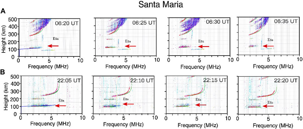
FIGURE 10. Ionograms from Digisonde located at Santa Maria station, which detected Esa layers only between 06:20 UT - 06:35 UT panel (A), and 22:05 UT - 22:20 UT panel (B) on September, 25. The red arrows show the Es_a layer presence, and the blue line (6:20 UT and 22:05 UT) is referent the critical modeled frequency (MHz) altitude.

FIGURE 11

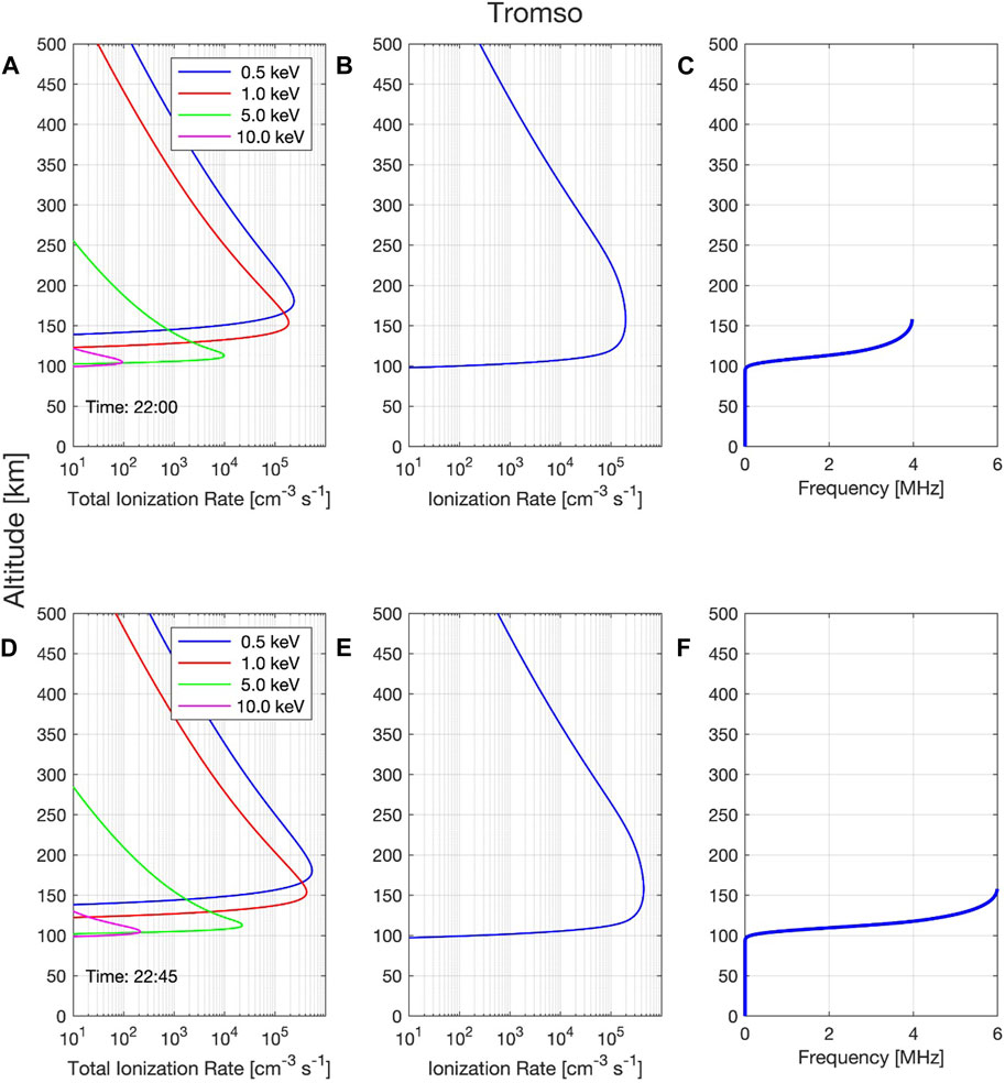
FIGURE 11. Ionization rate altitude profiles panels (A,D); ionization rate altitude integrated panels (B,E); and frequency range altitude for Tromso station panels (C,F) at 22:00 UT and 22:45 UT on 25 September 2017.

The ionization rate altitude profiles, ionization rate altitude integrated, and frequency range altitude to Tromso station are presented in Figure 11. The time of analysis is 22:00 UT (panels a, b and c) on 25 September 2017, to compare with the results observed in Santa Maria station at 22:05 UT (Figures 9D, E, F). Although the dynamic mechanisms that cause the EP over Tromso to be different from the mechanisms over SAMA, at the ionosphere, the formation mechanism of Esa layer in both regions has the EP as a main ingredient. It means that the electron energy levels, and the values of the ionization rate define the characteristics of the Esa layers in both regions, such as the Esa layer base height and the maximum frequency reached by Esa layer. Figure 9B (first panels) and Supplementary Figure S5 (top panel - Supporting Information) show that the Esa layer base height in Santa Maria is close to 100 km of altitude and in Tromso is >130 km of altitude, respectively, while the maximum frequency reached by Esa layer in Santa Maria is > 3 MHz and in Tromso is ∼ 4 MHz.

8 Concluding remarks

The dynamic mechanisms inside the inner radiation belt, generally under the influence of the solar wind structures, can cause the low-energy EP (0.5 keV–10 keV) into the atmosphere (100–200 km) over the SAMA region. The pitch angle scattering driven by plasmaspheric hiss waves is responsible for this range of EP in this altitude over this region, which generally contributes to the generation of the Esa layer during the recovery phase period of the geomagnetic storm, associated with ICMEs (Batista and Abdu, 1977; Moro et al., 2022a; Da Silva et al., 2022).

The environment here is under the influence of an HSS. This solar wind structure triggered the dynamic mechanisms able to cause the low-energy electron injections (seed and source populations) inside the radiation belts, followed by the low-energy EP in the auroral and SAMA region. These dynamic mechanisms also contributed to generating the plasma waves inside the radiation belts under the influence of the Alfvenic fluctuations. Although the substorms driven by this HSS were considered weak, the total ionization rate altitude profiles in Santa Maria station presented significant energy levels between 0.5 and 10 keV, which are greater than the energy levels showed in Tromso station and presented by Da Silva et al. (2022) Santa Maria station. It means that the level of low-energy electron precipitation (EP) predominant defines the base height of the Esa layer, which is close to 100 km at Santa Maria station and 130 km at Tromso station. Additionally, the ionization rate integrated defines the maximum critical frequency of the Esa layer, which reached values > 3 MHz in Santa Maria and ∼ 4 MHz in Tromso. This behavior suggests that the storm’s intensity is not crucial to define the EP levels over the SAMA region once the Esa layers were generated without high values of the AE index.

Therefore, the main ingredients responsible for generating the Esa layer over the SAMA region are related directly to the total and integrated ionization rate at the interest’s altitude. They are essential to define the base height and the maximum critical frequency of the Esa layer. Thereby, it is important to highlight that they are dependent on several factors, such as the amount, period, and levels of the electron flux injections in the inner radiation belt, the power spectral density of the hiss waves, the period of the hiss wave activities, and the resonance condition, which can have different behaviors under the influence of the different solar wind structures.

Data availability statement

The datasets presented in this study can be found in online repositories. The names of the repository/repositories and accession number(s) can be found in the article/Supplementary Material. All the data used are available at: ECT: https://cdaweb.gsfc.nasa.gov/pub/data/rbsp/ EMFISIS: https://emfisis.physics.uiowa.edu/Flight ACE: http://www.srl.caltech.edu/ACE/ASC/DATA/browse-data Digisonde (Santa Maria): http://www2.inpe.br/climaespacial/portal/ionossondas-inicio/ Digisonde (Tromso): https://lgdc.uml.edu/common/DIDBYearListForStation?ursiCode=TR169 IGRF-13: https://www.ngdc.noaa.gov/geomag/calculators/igrfgridForm.shtml VAP-AB orbit and foot print: https://sscweb.gsfc.nasa.gov/cgi-bin/Locator.cgi.

Author contributions

LS: Develop the idea of the article; make Figures 1, 4, 5; Supplementary Figure S1 and write all sections. JS: Revision of the manuscript and discussions about the results. LV. Runs the ionization rate model (make Figures 8, 9, 11; Supplementary Figures S4, S5, S6). OA: Calculate the electron lifetime based on the hiss model (make Figure 7). LR: Make Figure 2; Supplementary Figure S2, revision of the manuscript, and discussions about the Esa layers over SAMA. LA: Calculate the resonance kinetic energy (Make Figure 6; Supplementary Figure S3). DS: Revision of the manuscript and discussions about the results. VD: Revision of the manuscript and discussions about the results. JPM: Revision of the manuscript and discussions about the results. SC: Make Figure 3. JM: Download the data for making Figure 2; Supplementary Figure S2, revision of the manuscript, and discussions about the Esa layer over the SAMA region. CA: Revision of the manuscript and discussions about the results. CW: Revision of the manuscript and discussions about the results. VA: Discuss the atmospheric Wind conditions and their influences on Es layers over SAMA. HL: Revision of the manuscript and discussions about the results. ZL: Revision of the manuscript and discussions about the results. All authors contributed to the article and approved the submitted version.

Funding

This research was supported by the International Partnership Program of Chinese Academy of Sciences (grants 183311KYSB20200003 and 183311KYSB20200017). OA was supported by NASA grants 80NNSC19K0264, 80NNSC19K0848, 80NSSC20K0218, 80NSSC22K0522, and NSF grant 1914670. LV was supported by CNPq/MCTIC (Grant 307404/2016-1), TED-004/2020-AEB and PO-20VB.0009. LA was supported by CNPq/MCTIC (Grant 301476/2018-7).

Acknowledgments

LS, JM, LR, and VA are grateful for financial support from China-Brazil Joint Laboratory for Space Weather (CBJLSW), National Space Science Center (NSSC), and the Chinese Academy of Science (CAS). LS also thanks the autoplot platform. We acknowledge the NASA Van Allen Probes, Harlan E. Spence [PI ECT; University of New Hampshire] and Craig Kletzing [PI EMFISIS; University of Iowa] for use of data. We acknowledge the NASA ACE satellite, Edward Stone [PI ACE; Caltech]. LV thanks CNPq/MCTIC (Grant 307404/2016-1), TED-004/2020-AEB and PO-20VB.0009. LA thanks to CNPq/MCTIC (Grant 301476/2018-7).

Conflict of interest

The authors declare that the research was conducted in the absence of any commercial or financial relationships that could be construed as a potential conflict of interest.

Publisher’s note

All claims expressed in this article are solely those of the authors and do not necessarily represent those of their affiliated organizations, or those of the publisher, the editors and the reviewers. Any product that may be evaluated in this article, or claim that may be made by its manufacturer, is not guaranteed or endorsed by the publisher.

Supplementary material

The Supplementary Material for this article can be found online at: https://www.frontiersin.org/articles/10.3389/fspas.2023.1197430/full#supplementary-material

References

Alves, L. R., Alves, M. E. S., da Silva, L. A., Deggeroni, V., Jauer, P. R., and Sibeck, D. G. (2023). Relativistic kinematic effects in the interaction time of whistler-mode chorus waves and electrons in the outer radiation belt. Ann. Geophys. Discuss. doi:10.5194/angeo-2023-6

CrossRef Full Text | Google Scholar

Andrioli, V., Clemesha, B., Batista, P., and Schuch, N. (2009). Atmospheric tides and mean winds in the meteor region over Santa Maria (29.7°S; 53.8°W). J. Atmos. Solar-Terrestrial Phys. 71 (17-18), 1864–1876. doi:10.1016/j.jastp.2009.07.005

CrossRef Full Text | Google Scholar

Baker, D. N., Blake, J. B., Callis, L. B., Cummings, J. R., Hovestadt, D., Klecker, B. S., et al. (1994). Relativistic electron acceleration and decay time scales in the inner and outer radiation belts: SAMPEX. Geophys. Res. Lett. 21, 409–412. doi:10.1029/93GL03532

CrossRef Full Text | Google Scholar

Batista, I. S., and Abdu, M. A. (1977). Magnetic storm associated delayed sporadic E enhancements in the Brazilian Geomagnetic Anomaly. J. Geophys. Res. 82 (29), 4777–4783. doi:10.1029/JA082i029p04777

CrossRef Full Text | Google Scholar

Bittencourt, J. A. (1995). Fundamentals of plasma Physics. Edition 3. New York, NY: Springer. doi:10.1007/978-1-4757-4030-1

CrossRef Full Text | Google Scholar

Blake, J. B., Carranza, P. A., Claudepierre, S. G., Clemmons, J. H., Crain, W. R., Dotan, Y., et al. (2013). The magnetic electron ion spectrometer (MagEIS) instruments aboard the radiation belt storm probes (RBSP) spacecraft. Space Sci. Rev. 179, 383–421. doi:10.1007/s11214-013-9991-8

CrossRef Full Text | Google Scholar

Cai, H.-T., and Ma, S.-Y. (2007). Initial study of inversion method for estimating energy spectra of auroral precipitating particles from ground-based is radar observations. Chin. J. Geophys. 50 (1), 12–21. doi:10.1002/cjg2.1005

CrossRef Full Text | Google Scholar

Chulliat, A., Brown, W., Alken, P., Beggan, C., Nair, M., Cox, G., et al. (2020). The US/UK world magnetic model for 2020-2025: technical report. Great Britain, United States: NOAA. doi:10.25923/ytk1-yx35

CrossRef Full Text | Google Scholar

Claudepierre, S. G., O'Brien, T. P., Blake, J. B., Fennell, J. F., Roeder, J. L., Clemmons, J. H., et al. (2015). A background correction algorithm for Van Allen Probes MagEIS electron flux measurements. J. Geophys. Res. Space Phys. 120, 5703–5727. doi:10.1002/2015JA021171

CrossRef Full Text | Google Scholar

Da Silva, L. A., Shi, J., Alves, L. R., Sibeck, D., Marchezi, J. P., Medeiros, C., et al. (2021b). High-energy electron flux enhancement pattern in the outer radiation belt in response to the Alfvenic fluctuations within high-speed solar wind stream: a statistical analysis. J. Geophys. Res. Space Phys. 126. doi:10.1029/2021JA029363

CrossRef Full Text | Google Scholar

Da Silva, L. A., Shi, J., Alves, L. R., Sibeck, D., Souza, V. M., Marchezi, J. P., et al. (2021a). Dynamic mechanisms associated with high-energy electron flux dropout in the Earth's outer radiation belt under the influence of a coronal mass ejection sheath region. J. Geophys. Res. Space Phys. 126, e2020JA028492. doi:10.1029/2020JA028492

CrossRef Full Text | Google Scholar

Da Silva, L. A., Shi, J., Resende, L. C. A., Agapitov, O. V., Alves, L. R., Batista, I. S., et al. (2022). The role of the inner radiation belt dynamic in the generation of auroral-type sporadic E-layers over south American magnetic anomaly. Front. Astronomy Space Sci. 9, 1–23. doi:10.3389/fspas.2022.970308

CrossRef Full Text | Google Scholar

Da Silva, L. A., Sibeck, D., Alves, L. R., Souza, V. M., Jauer, P. R., Claudepierre, S. G., et al. (2019). Contribution of ULF wave activity to the global recovery of the outer radiation belt during the passage of a high-speed solar wind stream observed in September 2014. J. of Geophys. Research-Space Phys. 124, 1660–1678. doi:10.1029/2018ja026184

CrossRef Full Text | Google Scholar

Fang, X., Randall, C. E., Lummerzheim, D., Wang, W., Lu, G., Solomon, S. C., et al. (2010). Parameterization of monoenergetic electron impact ionization. Geophys. Res. Lett. 37, L22106. doi:10.1029/2010GL045406

CrossRef Full Text | Google Scholar

Funsten, H. O., Skoug, R. M., Guthrie, A. A., MacDonald, E. A., Baldonado, J. R., Harper, R. W., et al. (2013). Helium, oxygen, proton, and electron (HOPE) mass spectrometer for the radiation belt storm probes mission. Space Sci. Rev. 179, 423–484. doi:10.1007/s11214-013-9968-7

CrossRef Full Text | Google Scholar

Gabrielse, C., Angelopoulos, V., Runov, A., and Turner, D. L. (2014). Statistical characteristics of particle injections throughout the equatorial magnetotail. J. Geophys. Res. Space Phys. 119, 2512–2535. doi:10.1002/2013JA019638

CrossRef Full Text | Google Scholar

Green, A., Li, W., Ma, Q., Shen, X. C., Bortnik, J., and Hospodarsky, G. B. (2020). Properties of lightning generated whistlers based on Van Allen Probes observations and their global effects on radiation belt electron loss. Geophys. Res. Lett. 47 (17), e2020GL089584. doi:10.1029/2020GL089584

CrossRef Full Text | Google Scholar

Gurnett, D. A., and O'Brien, B. J. (1964). High-latitude geophysical studies with satellite Injun 3: 5. Very-low-frequency electromagnetic radiation. J. Geophys. Res. 69 (1), 65–89. doi:10.1029/JZ069i001p00065

CrossRef Full Text | Google Scholar

Hartley, D. P., and Denton, M. H. (2014). Solving the radiation belt riddle. Astronomy Geophys. 55 (6), 17–20. doi:10.1093/astrogeo/atu247

CrossRef Full Text | Google Scholar

Helliwell, R. A. (1965). Whistlers and related ionospheric phenomena. Stanford University Press.

Google Scholar

Horne, R. B., Lam, M. M., and Green, J. C. (2009). Energetic electron precipitation from the outer radiation belt duringgeomagnetic storms. Geophys. Res. Lett. 36, L19104. doi:10.1029/2009GL040236

CrossRef Full Text | Google Scholar

Hua, M., Li, W., Ni, B. B., Ma, Q. L., Green, A., Shen, X. C., et al. (2020). Very-low-frequency transmitters bifurcate energetic electron belt in near-Earth space. Nat. Commun. 11, 4847. doi:10.1038/s41467-020-18545-y

PubMed Abstract | CrossRef Full Text | Google Scholar

Khazanov, G. V., and Ma, Q. (2021). Dayside low energy electron precipitation driven by hiss waves in the presence of ionospheric photoelectrons. J. Geophys. Res. Space Phys. 126, e2021JA030048. doi:10.1029/2021JA030048

CrossRef Full Text | Google Scholar

Kletzing, C. A., Kurth, W. S., Acuna, M., MacDowall, R. J., Torbert, R. B., Averkamp, T., et al. (2013). The electric and magnetic field instrument suite and integrated science (EMFISIS) on RBSP. Space Sci. Rev. 179 (1–4), 127–181. doi:10.1007/s11214-013-9993-6

CrossRef Full Text | Google Scholar

Lemaire, J. (1975). The mechanics of formation of the plasmapause. Ann. Geophys. 31 (1), 175–189.

Google Scholar

Li, W., Ma, Q., Thorne, R. M., Bortnik, J., Kletzing, C. A., Kurth, W. S., et al. (2015). Statistical properties of plasmaspheric hiss derived from Van Allen Probes data and their effects on radiation belt electron dynamics. J. Geophys. Res. Space Phys. 120 (5), 3393–3405. doi:10.1002/2015JA021048

CrossRef Full Text | Google Scholar

Li, W., Shen, X.-C., Ma, Q., Capannolo, L., Shi, R., Redmon, R. J., et al. (2019). Quantification of energetic Electron precipitation driven by plume whistler mode waves, Plasmaspheric hiss, and exohiss. Geophys. Res. Lett. 46, 3615–3624. doi:10.1029/2019GL082095

CrossRef Full Text | Google Scholar

Li, Y. X., Yue, C., Liu, Y., Zong, Q.-G., Zou, H., and Ye, Y. G. (2023). Dynamics of the inner electron radiation belt: a review. Earth Planet. Phys. 7 (1), 109–118. doi:10.26464/epp2023009

CrossRef Full Text | Google Scholar

Mauk, B. H., Fox, N. J., Kanekal, S. G., Kessel, R. L., Sibeck, D. G., and Ukhorskiy, A. (2013). Science objectives and rationale for the radiation belt storm probes mission. Space Sci. Rev. 179 (1–4), 3–27. doi:10.1007/s11214-012-9908-y

CrossRef Full Text | Google Scholar

Meredith, N. P., Horne, R. B., Thorne, R. M., Summers, D., and Anderson, R. R. (2004). Substorm dependence of plasmaspheric hiss. J. Geophys. Res. Space Phys. 109 (A6), 6209. doi:10.1029/2004JA010387

CrossRef Full Text | Google Scholar

Meredith, N. P., Horne, R. B., Lam, M. M., Denton, M. H., Borovsky, J. E., and Green, J. C. (2011). Energetic electron precipitation during high-speed solar wind stream driven storms. J. Geophys. Res. 116 (A5), A05223. doi:10.1029/2010JA016293

CrossRef Full Text | Google Scholar

Moro, J., Xu, J., Denardini, C. M., Resende, L. C. A., Silva, L. A., Chen, S. S., et al. (2022a). Different sporadic-E (Es) layer types development during the August 2018 geomagnetic storm: evidence of auroral type (Es) over the SAMA region. J. of Geophys. Research-Space Phys. V., 1. doi:10.1029/2021JA029701

CrossRef Full Text | Google Scholar

Moro, J., Xu, J., Denardini, C. M., Stefani, G., Resende, L. C. A., Santos, A. M., et al. (2022b). Blanketing sporadic-E layer occurrences over Santa Maria, A transition station from low to middle latitude in the South American magnetic anomaly (sama). J. Geophys. Research-Space Phys. 127, E2022ja030900. doi:10.1029/2022ja030900

CrossRef Full Text | Google Scholar

Nikolaeva, V., Gordeev, E., Sergienko, T., Makarova, L., and Kotikov, A. (2021). AIM-E: E-region auroral ionosphere model. Atmosphere 12, 748. doi:10.3390/atmos12060748

CrossRef Full Text | Google Scholar

Pinto, O., and Gonzalez, W. D. (1989). Energetic electron precipitation at the South atlantic magnetic anomaly: a review. J. Atmos. Terr. Phys. 51 (5), 351–365. doi:10.1016/0021-9169(89)90117-7

CrossRef Full Text | Google Scholar

Rees, M. H. (1963). Auroral ionization and excitation by incident energetic electrons. Planet. Space Sci. 11 (10), 1209–1218. doi:10.1016/0032-0633(63)90252-6

CrossRef Full Text | Google Scholar

Reeves, G. D., Friedel, R. H. W., Larsen, B. A., Skoug, R. M., Funsten, H. O., laudepierre, S. G., et al. (2016). Energy-dependent dynamics of keV to MeV electrons in the inner zone, outer zone, and slot regions. J. Geophys. Res. Space Phys. 121 (1), 397–412. doi:10.1002/2015JA021569

PubMed Abstract | CrossRef Full Text | Google Scholar

Resende, L. C. A., Zhu, Y., Arras, C., Denardini, C. M., Chen, S. S., Moro, J., et al. (2022b). Analysis of the sporadic-E layer behavior in different American stations during the days around the september 2017 geomagnetic storm. Atmosphere 13, 1714. doi:10.3390/atmos13101714

CrossRef Full Text | Google Scholar

Resende, L. C. A., Zhu, Y., Denardini, C. M., Moro, J., Arras, C., Chagas, R. A. J., et al. (2022c). Worldwide study of the Sporadic E (Es) layer development during a space weather event. J. Atmos. Solar-Terrestrial Phys. 241, 105966. doi:10.1016/j.jastp.2022.105966

CrossRef Full Text | Google Scholar

Rodger, C. J., Clilverd, M. A., Seppälä, A., Thomson, N. R., Gamble, R. J., Parrot, M., et al. (2010). Radiation belt electron precipitation due to geomagnetic storms: significance to middle atmosphere ozone chemistry. J. Geophys. Res. 115, A11320. doi:10.1029/2010JA015599

CrossRef Full Text | Google Scholar

Roederer, J. G. (1967). On the adiabatic motion of energetic particles in a model magnetosphere. J. Geophys. Res. 72 (3), 981–992. doi:10.1029/jz072i003p00981

CrossRef Full Text | Google Scholar

Santolík, O., Parrot, M., and Lefeuvre, F. (2003). Singular value decomposition methods for wave propagation analysis. Radio Sci. 38 (1), 1010. doi:10.1029/2000RS002523

CrossRef Full Text | Google Scholar

Sarris, E. T., Krimigis, S. M., and Armstrong, T. P. (1976). Observations of magnetospheric bursts of high-energy protons and electrons at ∼35R_Ewith Imp 7. J. Geophys. Res. 81 (13), 2341–2355. doi:10.1029/JA081i013p02341

CrossRef Full Text | Google Scholar

Shi, R., Summers, D., Ni, B., Fennell, J. F., Blake, J. B., Spence, H. E., et al. (2016). Survey of radiation belt energetic electron pitch angle distributions based on the Van Allen Probes MagEIS measurements. J. Geophys. Res. Space Phys. 121, 1078–1090. doi:10.1002/2015JA021724

CrossRef Full Text | Google Scholar

Stone, E. C., Frandsen, A. M., Mewaldt, R. A., Christian, E. R., Margolies, D., Ormes, J. F., et al. (1998). The advanced composition explorer. Space Sci. Rev. 86 (1/4), 1–22. doi:10.1023/A:1005082526237

CrossRef Full Text | Google Scholar

Su, Z., Liu, N., Zheng, H., Wang, Y., and Wang, S. (2018). Large-amplitude extremely low frequency hiss waves in plasmaspheric plumes. Geophys. Res. Lett. 45 (2), 565–577. doi:10.1002/2017GL076754

CrossRef Full Text | Google Scholar

Takahashi, K., Lee, D.-H., Nosé, M., Anderson, R. R., and Hughes, W. J. (2003). CRRES electric field study of the radial mode structure of Pi2 pulsations. J. Geophys. Res. 108 (A5), 1210. doi:10.1029/2002JA009761

CrossRef Full Text | Google Scholar

Thomas, N., Shiokawa, K., Miyoshi, Y., Kasahara, Y., Shinohara, I., Kumamoto, A., et al. (2021). Investigation of small scale electron density irregularities observed by the Arase and Van Allen Probes satellites inside and outside the plasmasphere. J. Geophys. Res. Space Phys. 126, e2020JA027917. doi:10.1029/2020JA027917

CrossRef Full Text | Google Scholar

Tsyganenko, N. A., and Sitnov, M. I. (2005). Modeling the dynamics of the inner magnetosphere during strong geomagnetic storms. J. Geophys. Res. 110, A03208. doi:10.1029/2004JA010798

CrossRef Full Text | Google Scholar

Turner, D. L., Claudepierre, S. G., Fennell, J. F., O'Brien, T. P., Blake, J. B., Lemon, C., et al. (2015). Energetic electron injections deep into the inner magnetosphere associated with substorm activity. Geophys. Res. Lett. 42 (7), 2079–2087. doi:10.1002/2015GL063225

CrossRef Full Text | Google Scholar

Vampola, A. L., and Korth, A. (1992). Electron drift echoes in the inner magnetosphere. Geophys. Res. Lett. 19, 625–628. doi:10.1029/92GL00121

CrossRef Full Text | Google Scholar

Whitehead, J. D. (1970). Production and prediction of sporadic E. Rev. Geophys. 8 (1), 65–144. doi:10.1029/RG008i001p00065

CrossRef Full Text | Google Scholar

Xiang, Z., Li, X. L., Selesnick, R., Temerin, M. A., Ni, B. B., Zhao, H., et al. (2019). Modeling the quasi-trapped electron fluxes from cosmic ray albedo neutron decay (CRAND). Geophys. Res. Lett. 46 (4), 1919–1928. doi:10.1029/2018GL081730

CrossRef Full Text | Google Scholar

Xiao, F., Zong, Q.-G., and Chen, L. (2009). Pitch-angle distribution evolution of energetic electrons in the inner radiation belt and slot region during the 2003 Halloween storm. J. Geophys. Res. 114, A01215. doi:10.1029/2008JA013068

CrossRef Full Text | Google Scholar

Zhang, Z. X., Xiang, Z., Wang, Y. F., Ni, B. B., and Li, X. Q. (2021). Electron acceleration by magnetosonic waves in the deep inner belt (L = 1.5-2) region during geomagnetic storm of August 2018. J. Geophys. Res. Space Phys. 126 (12), e2021JA029797. doi:10.1029/2021JA029797

CrossRef Full Text | Google Scholar

Zhao, H., Li, X., Blake, J. B., Fennell, J. F., Claudepierre, S. G., Baker, D. N., et al. (2014). Peculiar pitch angle distribution of relativistic electrons in the inner radiation belt and slot region. Geophys. Res. Lett. 41 (7), 2250–2257. doi:10.1002/2014GL059725

CrossRef Full Text | Google Scholar