 Jesse Schneider
 David C. Stenning
 Lloyd T. Elliott
- Department of Statistics and Actuarial Science, Simon Fraser University, Burnaby, BC, Canada
Deep learning has increasingly been applied to supervised learning tasks in astronomy, such as classifying images of galaxies based on their apparent shape (i.e., galaxy morphology classification) to gain insight regarding the evolution of galaxies. In this work, we examine the effect of pretraining on the performance of the classical AlexNet convolutional neural network (CNN) in classifying images of 14,034 galaxies from the Sloan Digital Sky Survey Data Release 4. Pretraining involves designing and training CNNs on large labeled image datasets unrelated to astronomy, which takes advantage of the vast amounts of such data available compared to the relatively small amount of labeled galaxy images. We show a statistically significant benefit of using pretraining, both in terms of improved overall classification success and reduced computational cost to achieve such performance.
1 Introduction
Convolutional neural networks (CNNs) are a type of deep learning that is particularly well suited to computer vision tasks (Aggarwal, 2018). Originally inspired by research on the visual cortex by neurophysiologists Hubel and Wiesel in the mid-20th century (Hubel and Wiesel, 1959; Aggarwal, 2018), CNNs have been successfully applied to a variety of computer vision tasks, such as image classification (Krizhevsky et al., 2012), facial recognition (Taigman et al., 2014), and classification of various forms of interstitial lung disease (Li et al., 2014). CNNs have also been applied to tasks outside of computer vision, such as forecasting prices in financial stock markets (Tsantekidis et al., 2017).
As astronomy and astrophysics increasingly rely on large sets of image data, CNNs have increasingly been used to tackle a variety of interesting astronomical and astrophysical problems. These include identifying gravitational lenses (Davies et al., 2019), identifying contamination in astronomical images, e.g., by cosmic rays and diffraction spikes (Paillassa et al., 2020), and for supernovae detection (Cabrera-Vives et al., 2016). One particular task for which CNNs have proved successful, which will be discussed in more depth below, is galaxy morphology classification as in Cavanagh et al. (2021). We will therefore use galaxy morphology classification to explore how pretraining [a type of transfer learning (Tan et al., 2018; Ribani and Marengoni, 2019)] can potentially benefit many tasks in astronomy and astrophysics that use CNNs.
When applied to a particular task, CNNs (and neural networks in general) can be trained from scratch for the given task, or instead we can use a pretrained network. A pretrained CNN is one which has already been trained on a separate data set prior to its application to the given task (Aggarwal, 2018). The training of neural networks is, in general, an energy-intensive activity (Strubell et al., 2020; Borowiec et al., 2022), and research is ongoing to quantify and reduce energy use [e.g., (Yang et al., 2017; García-Martín et al., 2019)]. Training neural networks from scratch can require more training and therefore greater expense and resource usage compared to using a pretrained network. Furthermore, this requirement for a large amount of training presupposes the availability of a sufficient amount of data within the intended domain for the desired amount of training. Thus, data availability itself can be a limitation which may preclude the possibility of a large amount of training being performed from scratch.
In astronomy, obtaining large, labelled training data sets is expensive, impractical, or both. As a result of the demands required to train deep learning models from scratch, pretraining may be an attractive alternative for astronomy. In recent years, transfer learning has been adopted for classification tasks in astronomy and astrophysics involving galaxy morphologies (Domínguez Sánchez et al., 2018), variable stars (Kim et al., 2021), and star clusters (Wei et al., 2020). However, the learning that is “transferred” in these cases is between different astronomical surveys. That is, a classifier is trained using data from one survey, and deployed, perhaps with modification, on test data arising from a different survey. For example, a model may be trained on Sloan Digital Sky Survey images and deployed on Dark Energy Survey images (Domínguez Sánchez et al., 2018).
An alternative type of transfer learning, which we refer to specifically as pretraining hereafter, involves the practice of training a neural network on another unrelated data set before applying the neural network to the particular data set of interest. This means that pretraining, using our definition, can exploit the vast effort undertaken to design CNNs for classifying large volumes of natural (everyday) images. Specifically, we will use a CNN trained on millions of non-astronomical images that comprise the ImageNet database (Deng et al., 2009); this CNN is known as AlexNet (Krizhevsky et al., 2012). We will demonstrate, through a series of numerical experiments, that for the task of galaxy morphology classification, a pretrained AlexNet outperforms an architecturally identical CNN that is trained from scratch using only galaxy morphology images. Transfer learning using training on a large data set of natural images has been explored in the context of analysis of data from the Laser Interferometer Gravitational-Wave Observatory (George et al., 2018) and in galaxy merger detection (Ackermann et al., 2018). However, as far as we are aware, such transfer learning has not been explored in the context of galaxy morphology classification, which is the focus of the present paper.
The rest of this paper explores the utility of pretraining in the application of a CNN to galaxy morphology image classification. This domain represents a potential use case for a pretrained network due to the expense and difficulty of gathering and labeling images of galaxies (Cavanagh et al., 2021). We begin in Section 2 with an overview of galaxy morphology classification and the data we will use for our experiments. In Section 3 we describe CNNs, including the particular CNN used in this paper, as well as data preparation procedures and tooling. Our numerical experiments and results are detailed in Section 4. We discuss and summarize our contributions in Section 5, and also discuss directions for future research.
All code and materials necessary to reproduce our work can be found at: https://github.com/jsa378/01_masters.
2 Galaxy morphology classification and data
Images of galaxies are captured using either earthbound equipment or spacecraft. Traditionally, the images are classified by groups of experts who examine each image and come to a consensus regarding its classification (Cavanagh et al., 2021). In order to speed up the classification of images, other strategies have been used, such as the recruitment of enthusiastic amateurs (Lintott et al., 2010), and various automated classification techniques (Cheng et al., 2020).
CNNs in particular and deep learning more generally are well suited to tackle challenges in galaxy morphology classification, and as such there is a large body of literature devoted to such aims. We describe a few of these below, but note that the list is non-exhaustive.
• Cheng et al. (2020) use CNNs and other machine/deep learning techniques to classify galaxy images from the Sloan Digital Sky Survey Data Release 7 into two categories (i.e., they perform two-way classification)—elliptical and spiral—reporting a best overall accuracy of over 99%, achieved with a CNN.
• Barchi et al. (2020) combine data from Galaxy Zoo 1 (Lintott et al., 2010) and the Dark Energy Survey (Abbott et al., 2018) when performing galaxy morphology classification. Using deep learning, they also achieve an overall accuracy of over 99% for two-way classification. However, when a third class (barred galaxies) is added, overall accuracy drops to 82%.
• Gharat and Dandawate (2022) also use Galaxy Zoo data, but adopt an extended Hubble tuning fork classification scheme, which places galaxies into 10 categories. Using a CNN, they achieve a best overall accuracy of about 85%.
• Cavanagh et al. (2021) use galaxy images from Sloan Digital Sky Survey Data Release 4 (SDSS DR4) (York et al., 2000; Stoughton et al., 2002; Adelman-McCarthy et al., 2006), and compare the performance of different CNNs on three-way and four-way classification, reporting best overall accuracy results of 83% and 81%, respectively. The four-way classification task is especially interesting and important because the fourth class is for “irregular and miscellaneous” galaxies that do not belong to one of the other three classes.
In the near future, an expected deluge of data obtained by new spacecraft such as the European Space Agency’s Euclid will overwhelm available resources for classification by humans (Silva et al., 2018). This adds urgency to the search for accurate, rapid, automated classification techniques, such as those cited above, among others. However, the galaxy image data currently available for training deep learning models remains relatively small. Following Cavanagh et al. (2021), for this work we used 14,034 (labeled) galaxy images from the SDSS DR4 (York et al., 2000; Stoughton et al., 2002; Adelman-McCarthy et al., 2006); the data are described in detail in Nair and Abraham (2010). Each galaxy is labeled according to its morphology, or shape, as belonging to the class of:
1) elliptical galaxies, having a smooth, diffuse, and elliptical shape;
2) spiral galaxies, disk-like in appearance and with spiral arms;
3) lenticular galaxies, an intermediate class of galaxies between the elliptical and spiral categories; or
4) irregular + miscellaneous (Irr + Misc) galaxies, not meeting the membership criteria for any of the above three categories.
An example of each type of galaxy, taken from the set of 14,034, is presented in Figure 1. The 14,034 galaxy morphology images varied in size, but were often quite small—around 100 × 100 pixels, or 0.01 megapixel. The class breakdown of the images is as follows:
1) 2,738 images of elliptical galaxies (19.4% of the total),
2) 7,708 images of spiral galaxies (54.9% of the total),
3) 3,215 images of lenticular galaxies (22.9% of the total), and
4) 373 images of Irr + Misc galaxies (2.7% of the total).
While this is clearly a highly imbalanced data set as governed by the distribution of galaxies in the regions imaged, we did not attempt to correct for these imbalances because for this work we are only concerned with demonstrating the benefit of pretraining. Further discussion of class differences is in Subsection 4.1.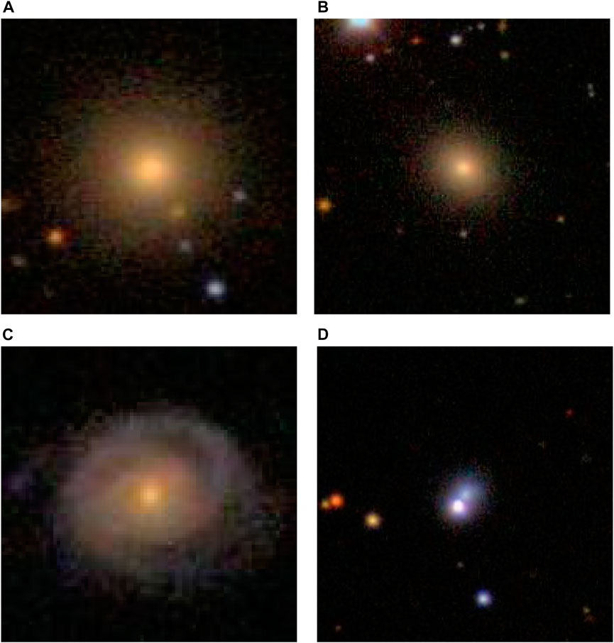
FIGURE 1. Examples of the four categories of galaxy from the Sloan Digital Sky Survey Data Release 4 (Nair and Abraham, 2010). (A) Elliptical galaxy. (B) Lenticular galaxy. (C) Spiral galaxy. (D) Irr + Misc galaxy.
Although Cavanagh et al. (2021) initially performed three-way classification, excluding Irr + Misc galaxies, we will limit the current work to considering the (more challenging) four-way classification task. The reason for this is two-fold: (1): we do not want to pre-filter Irr + Misc galaxies as they will undoubtedly be present in the future survey data, and (2) it is precisely for Irr + Misc galaxies that we notice the greatest benefit of pretraining, perhaps due to the relative lack of training examples; we will demonstrate and discuss this in more detail in Sections 4, 5.1
3 Methods and data preparation
3.1 Convolutional neural networks
3.1.1 Introduction to CNNs
CNNs are a type of neural network that are well suited to image data (Goodfellow et al., 2016). They are so named because of the “convolution” operations applied within the network, although strictly speaking these operations are cross-correlations (Goodfellow et al., 2016). CNNs are perhaps the archetypal example of biologically-inspired artificial intelligence, because their conception was influenced by exploration of the visual cortex in the mid-20th century (Aggarwal, 2018).
Although formal mathematical justification for CNNs is lacking, the common explanation is that CNNs function by detecting relatively crude features of an input image, such as lines, in the early layers of the network, and superimpose these features into progressively more complex features in later layers (Aggarwal, 2018).
3.1.2 CNN operations
Like feedforward neural networks, CNNs consist of an input layer, one or more hidden layers and an output layer. The primary differences are the types of operations that the layers perform. The fundamental principles of neural networks—the forwards and backwards phases, and gradient-based optimization—also apply to CNNs. Furthermore, training methods consisting of feeding the entire training data set to the network multiple times, each time referred to as an epoch, are similar for both types of networks. For brevity, therefore, we will focus on the unique mathematical operations employed in CNNs; these unique operations are convolution and pooling operations. We will also briefly discuss the regularization technique known as dropout, which is commonly used to avoid overfitting deep neural networks.
3.1.2.1 The convolution (cross-correlation)
Consider a color image I of size h × w pixels, represented numerically as an array with dimensions h × w × 3. (The depth of 3 is for storage of the red, green and blue color values.) The convolution operation involves placing a smaller h′ × w′ × 3 (h′ ≤ h, w′ ≤ w) array K, called the kernel or filter, at all possible positions overlaid on I and computing the component-wise dot product between I and K.2
More formally, the convolution of h × w × 3 image I (having i, j, l entry Ii,j,l) with h′ × w′ × 3 kernel K (having i, j, l entry Ki,j,l) is a function
defined by
3.1.2.2 The max pool
The max pool operation involves a smaller array P similar to the kernel K, except that P has a depth of 1. If P has dimensions p × q × 1 and acts on a layer L having dimensions h × w × d, then the pooling operation produces a layer P(L) having dimensions (h − p + 1) × (w − q + 1) × d. In particular,
3.1.2.3 Dropout
Dropout is a regularization technique applied layer-wise during CNN training, which involves training random subsets of the overall network (Hinton et al., 2012; Srivastava et al., 2014). If dropout is applied to layer l in the network, then each time the network is fed a training image, independent draws from a Bernoulli(p) distribution are made to determine which nodes in layer l are kept or discarded. The training prediction and backpropagation are then carried out only over the sub-network containing the remaining nodes. During training, repeated samples from the Bernoulli(p) distribution are drawn, which means that different subsets of the original network are trained. During testing, dropout is not applied, so the entire network is used. Using dropout significantly reduces network overfitting, and thus improves the network’s ability to generalize to the test data (Srivastava et al., 2014).
3.2 AlexNet
The CNN that underpins our work is called AlexNet (Krizhevsky et al., 2012). Although CNNs date back to the 1980s, in 2012 the AlexNet CNN ushered in what is arguably the modern era in computer vision by winning the ImageNet Large Scale Visual Recognition Challenge, thoroughly surpassing past performers and challengers (Aggarwal, 2018). Since then, CNNs have served as the standard for image classification, as can be seen by the fact that subsequent winners of the ImageNet competition have also been CNNs (Aggarwal, 2018). Below, a brief summary of the AlexNet architecture is provided. Further details can be found in Krizhevsky et al. (2012).
The AlexNet network can be broken into two broad parts: an early convolutional part and a later, more conventional feed-forward part. In the convolutional part, AlexNet takes as input a 224 × 224 × 3 image and, over a number of layers, applies an increasing number of convolution filters which decrease in height and width. The first convolutional layer applies 64 filters of size 11 × 11 × 3; a later convolutional layer applies 384 filters of size 3 × 3 × 256. (As previously mentioned, formal mathematical justification for CNN operation is lacking, but the intuition is that larger numbers of smaller filters in later layers capture more complex features of the input image.) AlexNet uses five convolutional layers in total. After every convolutional layer the ReLU operation is used, and a handful of max-pooling operations are layered in as well. In the feed-forward part, AlexNet contains 3 linear layers with ReLU activation functions before delivering its class probability calculations.3 To reduce overfitting, dropout is used.
Because the ImageNet Challenge requires classifying images belonging to one of 1,000 categories, AlexNet by default has 1,000 nodes in its final layer. However, this can be modified when applying AlexNet for other purposes, such as classifying galaxy morphology into four categories.
The architecture of AlexNet is shown in a standard visual representation in Figure 2. Note that the original AlexNet architecture (shown in Figure 2) has 1,000 nodes in its output layer, corresponding to the 1,000 object categories in the ImageNet dataset. For this paper, the number of output nodes was reduced to 4, in accordance with the number of categories of galaxy morphology.
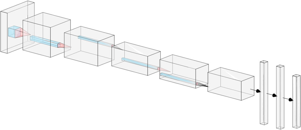
FIGURE 2. The AlexNet architecture. After receiving a 224 × 224 × 3 input image, AlexNet applies a sequence of convolutions, ReLU operations, and pooling operations (in the portions represented by the deep rectangular prisms) before applying a set of linear layers with dropout (in the portions represented by the tall rectangular prisms). Figure created using NN-SVG.
3.3 Data preparation, procedures and tooling
For our work, all galaxy images were scaled to 256 × 256 in height and width to allow room for cropping to 224 × 224, which is the input size required by AlexNet. Regarding data augmentation, PyTorch is naturally set up to use random data augmentation, which involves the probabilistic application of standard data augmentation techniques. For example, the PyTorch function transforms.RandomHorizontalFlip() will, each epoch, horizontally flip a given image with probability 0.5.
The data set was split into 12,000 training images and 2,034 testing images uniformly at random. We constructed 100 such test/train splits. No hyperparameter tuning was done. (The decision to forgo hyperparameter tuning was made in order to make an even comparison between the pretrained and non-pretrained networks.) For each random split of the data set, which we refer to as a run, the pretrained AlexNet was trained for 200 epochs, while the non-pretrained AlexNet was trained for 400 epochs. This additional training time was given to the non-pretrained AlexNet so that it had a better opportunity to achieve optimal performance. The training used the standard cross-entropy loss via the PyTorch function torch.nn.CrossEntropyLoss(), which is described in the PyTorch documentation.
Standard Python-language tools including Matplotlib (Hunter, 2007), NumPy (Harris et al., 2020), pandas (McKinney, 2010; Pandas development team, 2020), and seaborn (Waskom, 2021) were used for performing our numerical experiments and compiling the results to be presented. In particular, PyTorch (Paszke et al., 2019) was used to obtain the pretrained and non-pretrained AlexNet networks, and to train and test them. The networks used are available off the shelf in PyTorch, via the torchvision.models subpackage. Further, the Cedar computing system at Simon Fraser University, provisioned by the Digital Research Alliance of Canada and the BC DRI Group, was used to carry out the neural network training and testing. Specifically, we used an Intel Xeon Silver 4216 processor with 12 GB RAM, and a NVIDIA Tesla V100 32 GB GPU. The total computing time used to carry out the numerical experiments described in this work was 5.64 CPU months and 0.96 GPU months.
4 Results
In this section, we present and discuss the results obtained over the 100 runs, and compare the pretrained and non-pretrained networks on a variety of metrics. We begin with Figure 3, in which we present histograms of the peak test accuracy for all runs for both the pretrained and non-pretrained networks; this figure also provides the epoch in which peak test accuracy is achieved. We also compute the difference in peak test accuracy between the pretrained and non-pretrained networks, as well as the difference in the epoch number for which peak test accuracy was achieved for the two networks, and display the results in Figure 4. (For the latter calculation, only the first 200 epochs of training were considered for the non-pretrained network.) (Note that here and elsewhere in the paper, accuracy refers to the overall accuracy—the percentage of correct classifications out of the total.)
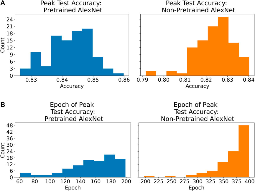
FIGURE 3. (A) Histograms of peak test accuracies for all runs for both the pretrained and non-pretrained networks. The pretrained networks are both more accurate on average and less varied in the peak accuracy that they achieve. (B) Histograms of the epoch in which peak test accuracy is achieved for each run, for both pretrained and non-pretrained networks. These histograms appear to suggest that 200 epochs of training are probably sufficient for the pretrained networks, while the non-pretrained networks might have benefited from even more than 400 epochs of training.
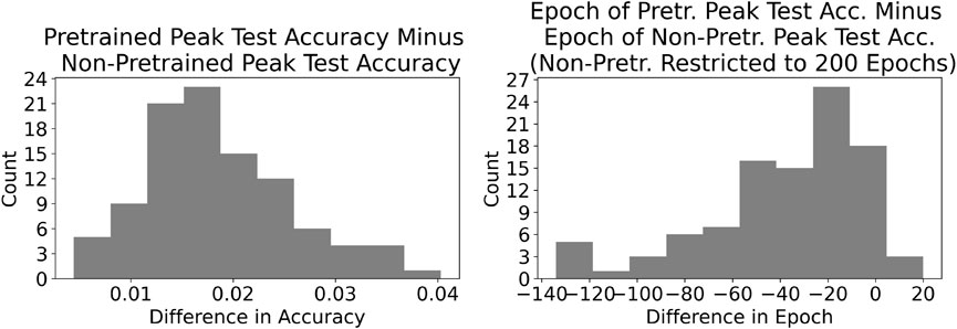
FIGURE 4. Histograms of the gains that result from using the pretrained network as opposed to the non-pretrained network. On the left is the peak test accuracy for the pretrained network minus the respective figure for the non-pretrained network. On the right is the epoch in which peak test accuracy was achieved for the pretrained network, minus the respective figure for the non-pretrained network, if the non-pretrained network had been restricted to train for only 200 epochs. It is clear that in terms of accuracy, the non-pretrained network never outperforms the pretrained network. In terms of speed in reaching peak accuracy, the pretrained network is almost always faster than the non-pretrained network, even when restricting the latter to 200 epochs of training.
To compare the pretrained and non-pretrained networks given a fixed training budget of 200 epochs, for each run we compute the difference between the peak accuracy of the pretrained network and the highest accuracy achieved by the non-pretrained network within its first 200 epochs of training. These results are presented in Figure 5. Examination of the histograms displayed in Figures 3–5 indicates that the pretrained AlexNet is preferred over the non-pretrained version. Pretraining leads to a higher overall accuracy, with an average peak accuracy (over the 100 runs) of 84.2% versus 82.4% for pretrained and non-pretrained, respectively. Furthermore, the pretrained network required significantly fewer epochs to reach its peak accuracy.
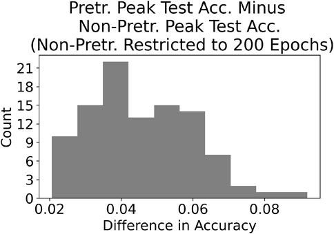
FIGURE 5. This figure is similar to the left histogram in Figure 4, except that we only consider the first 200 epochs for the non-pretrained networks. The advantage for the pretrained networks roughly doubles in this case.
To further explore the efficiency gain of pretraining, we evaluate the performance of the pretrained network over a restricted portion of training, such as the first 20 or 50 epochs. Selected results are presented in Figure 6. Figure 6A is a histogram of the difference in peak test accuracy for the 200-epoch pretrained network and the 50-epoch pretrained network, showing that the average gain in accuracy from the additional 150 epochs of training is only about 1%, and the maximum gain over all 100 runs is less than 3%. If the pretrained network is limited to only 20 epochs, then Figure 6B shows that the average gain in accuracy from the additional 180 epochs of training increases to approximately 2%–2.5%, with a maximum gain over the 100 runs of approximately 4%. This suggests that good performance can be achieved with relatively few epochs, such as 20. Depending on the specific application and resource constraints, it may therefore be sufficient to train a pretrained network for a relatively small number of epochs.
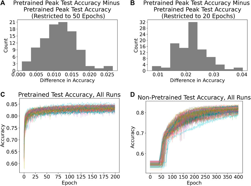
FIGURE 6. (A) Gain from letting the pretrained networks train for 200 epochs, as opposed to only 50 epochs. The gain is roughly 1%. (B) Gain from letting the pretrained networks train for 200 epochs, as opposed to only 20 epochs. The gain is roughly 2%–2.5%. (C) Each line in this panel contains the progression in test accuracy for the pretrained AlexNet for 1 of the 100 runs performed. It is clear that most of the improvement occurs within the first 20–30 epochs of training. (D) Each line in this panel contains the progression in test accuracy for the non-pretrained AlexNet for 1 of the 100 runs performed. The width of the band of lines suggests that performance of the non-pretrained AlexNet is more variable than the pretrained AlexNet. Furthermore, it usually takes around 50 epochs of training for the non-pretrained AlexNet’s parameters to adjust enough in order for the network’s predictions to begin shifting.
The bottom row of Figure 6 displays the test classification accuracy curves for pretrained (Figure 6C) and non-pretrained (Figure 6D) models over all 100 runs. The classification accuracy curves for the pretrained network reinforce the finding that the vast majority of improvement is acquired within the first 10–20 epochs of training. The widths of the bands of lines (an informal measure of variability) indicate that there is much less variability when using a pretrained model than when using a non-pretrained model. Figure 6D shows that the non-pretrained models require roughly 50 epochs of training in order to make any improvement at all; presumably this is the typical amount of training necessary to adjust a model’s parameters sufficiently in order to begin changing its classification behavior.
Table 1 provides a summary of the results presented in Figures 3–6. The information presented in the Table is consistent with that conveyed in the Figures, namely, that the pretrained network is more accurate and less variable in its performance than the non-pretrained network. Table 1 also provides more precise insight into the diminishing returns from training the pretrained network. Within the first 10% of training (20 epochs as opposed to 200), the pretrained network achieves an average peak test accuracy of 82.0%; within the first 25% of training (50 epochs), the pretrained network achieves a peak test accuracy of 83.1%. These means are within approximately 2% and 1%, respectively, of the peak test accuracy of 84.2%, and it is worth noting that despite the reduced training time, the standard deviations are essentially indistinguishable from those for the full 200 epochs’ worth of training. This implies that there is no (or very little) variance penalty when doing a comparatively small amount of training of the pretrained network.
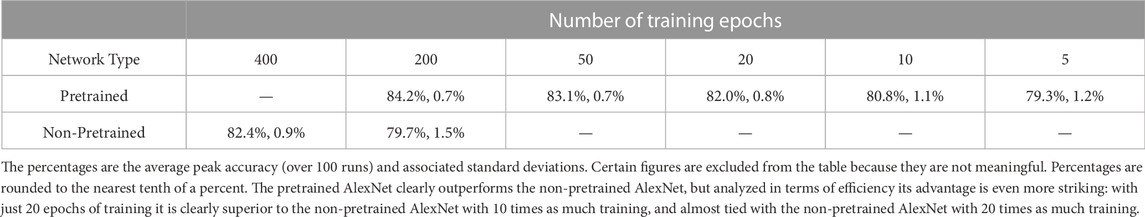
TABLE 1. Selected figures summarizing the results from the present paper.
Figure 7 is presented as typical output for one of the 100 runs for both networks. (Run 49 was selected arbitrarily.) The upper panels present the train and test accuracy progression over all epochs of training, while the lower panels present train and test performance for both networks over all epochs from the perspective of the loss function. In general, the values of the loss function did not appear to provide any information not already apparent from the accuracy information, but the loss information is nevertheless presented in Figure 7 for additional illustration.
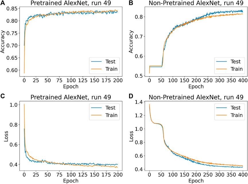
FIGURE 7. (A) Train and test accuracies of run 49 over all epochs for the pretrained AlexNet. The blue line in this panel is one of the lines in Figure 6C. (B) Equivalent information is presented for the non-pretrained AlexNet. The blue line in this panel is one of the lines in Figure 6D. (C) Train and test loss values of run 49 over all epochs for the pretrained AlexNet. (D) Equivalent information is presented for the non-pretrained AlexNet. Run 49 was chosen as an arbitrary representative of the 100 runs performed, although naturally there is some variation. Across most runs, performance of the pretrained network in training eventually surpasses performance in testing, although the point at which this occurs, and the eventual gap between the two, vary from run to run. This phenomenon is much weaker, perhaps nonexistent, for the non-pretrained networks, which may suggest that they would have benefited from more than 400 epochs of training. The non-pretrained networks also often take at least 50 epochs before the weights have adjusted enough for predictions to begin improving (Initially the non-pretrained networks appear to classify all test images as being of spiral galaxies).
4.1 Classification accuracies by class, and analysis of models
In order to develop a deeper understanding of model performance, the top-performing pretrained and non-pretrained models (by test accuracy) from each run were fed the test data set once again, and per-class accuracy figures were recorded. Figures 8, 9 display histograms of this result.
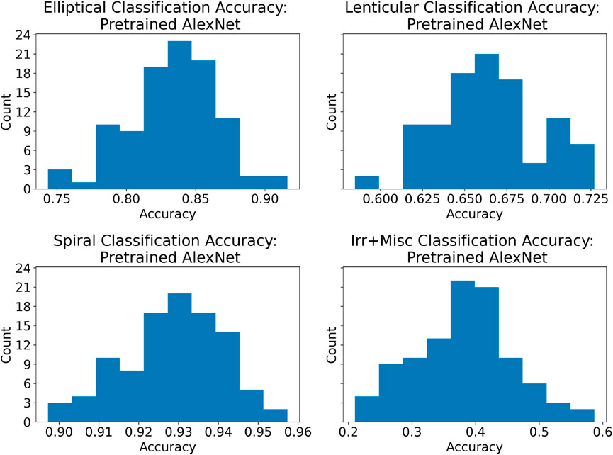
FIGURE 8. Histograms of class accuracies for the most accurate pretrained model of each run. There is a clear hierarchy in performance that is somewhat consistent with the distribution of the test data set (i.e., highest performance in the most frequently occurring images), although the fact that the lenticular galaxies are in some sense “between” the elliptical and spiral galaxies seems to reduce lenticular accuracy.
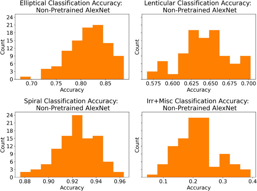
FIGURE 9. Histograms of class accuracies for the most accurate non-pretrained model of each run. These histograms are broadly similar to those in Figure 8, with the main exception being much poorer Irr + Misc performance.
The models were all roughly the same in that they were quite accurate when presented with images of spiral galaxies, less accurate when presented with images of elliptical galaxies, and less accurate still when presented with images of lenticular galaxies. Furthermore, they perform quite poorly when presented with images of irregular or miscellaneous galaxies, presumably due to the fact that there are few such images in the data set, and moreover the category itself is ill defined in the sense that it mostly serves as a grab-bag of images that fit in none of the preceding three categories.
However, besides the fact that pretrained networks classify images of elliptical, lenticular and spiral galaxies slightly more accurately than do the non-pretrained networks, there is one striking difference, namely, that the pretrained networks classify images of Irr + Misc galaxies almost twice as accurately as the non-pretrained networks. Even though the accuracy is still below 50%, this result might suggest that pretraining is potentially valuable for acquiring knowledge of uncommon or irregular examples in the application at hand. The fact that the pretrained networks offer a negligible improvement over the non-pretrained on spiral galaxies, by far the most common in the data set, might bolster this hypothesis.
Table 2 summarizes the results presented in Figures 8, 9. This Table makes clear that not only is the pretrained network superior across all classes to the non-pretrained network in average class accuracy, but the pretrained network is also less variable in its classification performance. The only exception to this is the Irr + Misc class, for which the pretrained network is more variable than the non-pretrained network, but the pretrained network’s almost twofold superiority in average accuracy for this class offsets its slightly higher variability.
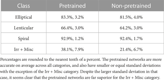
TABLE 2. Class accuracy averages and standard deviations across all 100 runs for both pretrained and non-pretrained networks.
Figure 10 presents confusion matrices for the top-performing pretrained and non-pretrained models from run 49. (This is the same run as that presented in Figure 7). The information in this figure is consistent with that presented in Figures 8, 9, namely, the hierarchy in classification performance across the four categories of galaxy morphology, and the general superiority of the pretrained network. However, the confusion matrices also provide some insight into the nature of the misclassifications made by the networks. In particular, both pretrained and non-pretrained models tend to misclassify galaxies into adjacent morphological categories. For example, the majority of the misclassified spiral galaxies are classified as lenticular, as opposed to being classified as elliptical galaxies.
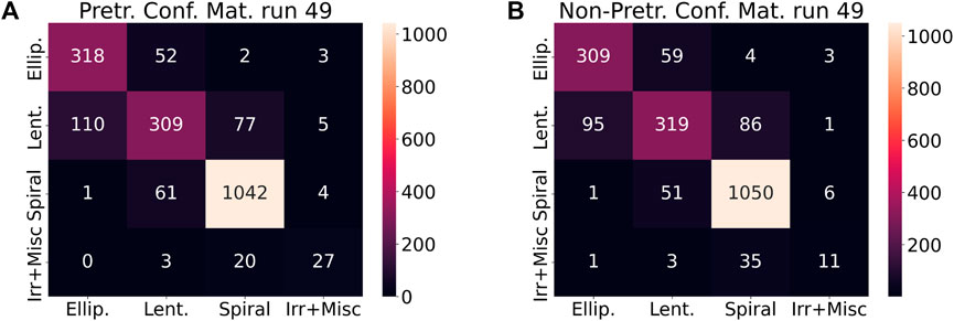
FIGURE 10. (A) Confusion matrix for the top-performing model from run 49 of the pretrained AlexNet. The sum of the numbers within a row is the number of images of that type within the test set for that run. For example, looking at the second row, in run 49 there were 110 + 309 + 77 + 5 = 501 images of lenticular galaxies in the test set, and 309/501 ≈ 61.7% of those images were classified correctly. Furthermore, 110/501 ≈ 22.0% of images of lenticular galaxies were mis-classified as elliptical galaxies. The confusion matrices for all runs are roughly similar in that the models tend to mis-classify images of galaxies into adjacent categories, which is relatively sensible. (B) Confusion matrix for the top-performing model from run 49 of the non-pretrained AlexNet. Again, the sum of the numbers within a row is the number of images of that type within the test set for that run. For example, looking at the second row, in run 49 there were 95 + 319 + 86 + 1 = 501 images of lenticular galaxies in the test set, and 319/501 ≈ 63.7% of those images were classified correctly. Furthermore, 95/501 ≈ 19.0% of images of lenticular galaxies were mis-classified as elliptical galaxies. As with the pretrained network, the confusion matrices for all runs are roughly similar in that the models tend to mis-classify images of galaxies into adjacent categories.
Figure 11 presents confusion matrix data over all 100 runs for the pretrained and non-pretrained AlexNets. (Note that as opposed to Figure 10, the totals have been converted to proportions). Similar to Figure 10, Figure 11 provides information not only concerning how the models classify images of galaxies, but also how they misclassify images of galaxies. In Figure 11A, the value in each cell of the matrix is the average value for that cell from the 100 individual confusion matrices for the pretrained network. Figure 11C contains an equivalent matrix for the non-pretrained network. Figures 11B, D contain the associated cell-wise standard deviations for the pretrained and non-pretrained networks, respectively. As with Figure 10, the most salient feature of Figure 11 is the demonstration that both pretrained and non-pretrained networks tend to misclassify images of galaxies into adjacent categories. This is sensible given that the morphological characteristics of these galaxies are thought to occur on a continuum, at least to some extent.
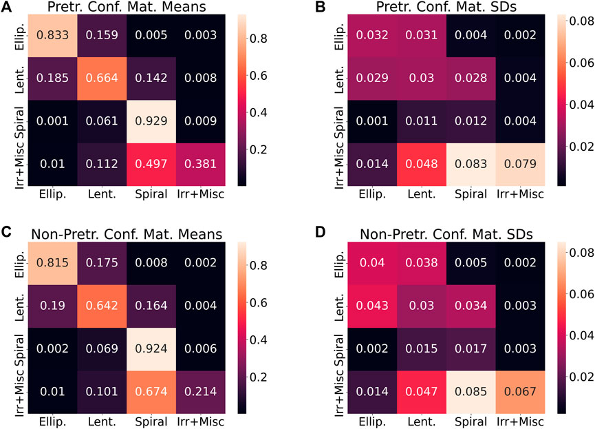
FIGURE 11. (A) The average confusion matrix for the pretrained AlexNet is shown. The entries in this confusion matrix are the means across all 100 confusion matrices for the pretrained network, one pertaining to each run. This figure shows that the network tends to misclassify images of galaxies into adjacent categories. (B) A matrix showing the standard deviations of the individual confusion matrices for the pretrained network over all 100 runs. (C) The average confusion matrix for the non-pretrained AlexNet. The entries in this confusion matrix are the means across all 100 confusion matrices for the non-pretrained network, one pertaining to each run. Like the top-left figure, the bottom-left figure shows that the non-pretrained network tends to misclassify images of galaxies into adjacent categories. (D) A matrix showing the standard deviations of the individual confusion matrices for the non-pretrained network over all 100 runs.
4.2 Statistical significance tests
In order to provide a quantitative measure of the differences in performance between the pretrained and non-pretrained AlexNets, sign tests are conducted below. [The sign test makes no assumptions about the distribution of the quantities being compared (Roussas, 1997)].
Let X0, X1, …, X99 be independent and identically distributed random variables with distribution function F, representing the distribution of peak test accuracy for the 100 runs of the pretrained AlexNet (over 200 epochs of training). Similarly, let Y0, Y1, …, Y99 be independent and identically distributed random variables with distribution function G, representing the distribution of peak test accuracy for the 100 runs of the non-pretrained AlexNet (over 400 epochs of training). We wish to test the hypothesis
The result of the two-sided sign test is a p-value of approximately 1.58 × 10⁻³⁰, which provides strong evidence against the null hypothesis. We therefore have statistically significant evidence that the pretrained model is more accurate, even though the differences in accuracy may appear slight.
We can perform a similar test on differences in training time and energy used, using the number of epochs of training required to reach peak test accuracy as a proxy. Using similar definitions as above, the result of a two-sided sign test is the same p-value of approximately 1.58 × 10⁻³⁰, which again provides strong evidence against the null hypothesis. We therefore have statistically significant evidence that the pretrained model is not only more accurate but also more efficient.
4.3 Persistence of improvement to increased number of training epochs
To test how well the non-pretrained network might perform if it were given more than 400 epochs of training, runs 45–49 were repeated (i.e., the same train and test data splits were used), and both the pretrained and non-pretrained networks were trained for 1,000 epochs, instead of 200 and 400 epochs, respectively. (Runs 45–49 were arbitrarily chosen; time and computational resource limitations prevent using 1,000 epochs for all 100 runs). Table 3 contains peak test accuracies (rounded to the nearest tenth of a percent) and the epoch in which the peak test accuracy occurred.
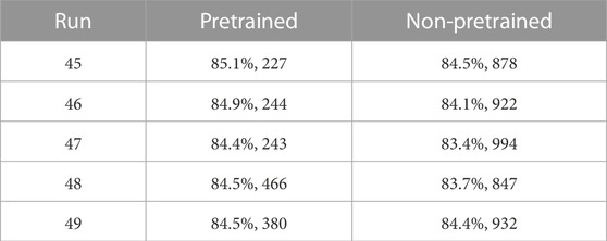
TABLE 3. Peak test accuracies (rounded to the nearest tenth of a percent) and the epoch in which the peak test accuracy occurred, using 1,000 epochs of training for runs 45–49.
Examining Table 3 we observe that, for each run, the pretrained network achieves a higher peak test accuracy than the non-pretrained network, and the difference is usually in the 0.5%–1.0% range. This evidence suggests that it is not simply a matter of increasing the training time for the non-pretrained network in order to close the gap to the pretrained network, at least not up to 1,000 epochs of training. In other words, Table 3 suggests that, at least up to 1,000 epochs of training, the advantage of pretraining on unrelated image data is not only greater efficiency but also greater ultimate performance in terms of overall accuracy.
5 Summary and outlook
The main objective of this work is to compare pretrained (on ImageNet) and non-pretrained versions of AlexNet by training them on galaxy images from the Sloan Digital Sky Survey Data Release 4 [as described in Nair and Abraham (2010)] and comparing their performance and efficiency. We note that while the overall classification accuracies achieved are comparable to or slightly surpass similar attempts [e.g., those described in Cavanagh et al. (2021)], chasing the highest possible classification accuracy would lead us to consider other network architectures, hyperparameter tuning, etc. Rather, we have demonstrated the benefit to considering pretrained deep learning models for certain tasks. Our results are as follows:
1. The pretrained AlexNet had a consistent edge (compared to the non-pretrained AlexNet) in peak classification accuracy. It had an 84.2% average peak test accuracy, compared to an average peak test accuracy of 82.4% for the non-pretrained AlexNet.
2. The pretrained AlexNet was much more efficient (compared to the non-pretrained AlexNet) in that it attained peak test accuracy much more quickly. On average, the pretrained AlexNet achieved peak test accuracy in epoch 155 (standard deviation of 34 epochs), compared to epoch 367 (standard deviation of 33 epochs) for the non-pretrained AlexNet.
3. When considering only the first 200 epochs of training for the non-pretrained AlexNet, in order to provide a comparison with the pretrained AlexNet given an equal amount of training, the peak classification accuracy advantage for the pretrained AlexNet more than doubles, to about 4.6%.
4. The pretrained AlexNet achieves comparable performance to state-of-the-art methods, such as Cavanagh et al. (2021), rather quickly. The pretrained AlexNet’s average peak test accuracy after just 20 epochs of training is 82.0%, comparable with the headline 81%–83% figures from Cavanagh et al. (2021). After 50 epochs of training, the pretrained AlexNet’s figure is 83.1%. This suggests that, taking advantage of pretraining, peak performance comparable to that from Cavanagh et al. (2021) can be achieved in as little as 10–60 min, depending on the computational resources at hand.
5. Regarding per-class accuracies, the most striking advantage for the pretrained AlexNet is that it often classifies the Irr + Misc images more than twice as accurately as the non-pretrained AlexNet. (Gains in classification accuracy for the other three categories are much smaller).
Regarding the last point, as a neural network is somewhat of a black box, it is hard to know precisely how the pretrained AlexNet becomes so much more adept at identifying images of Irr + Misc galaxies. It seems reasonable to speculate that there is some sort of generalizable information within the unrelated ImageNet (pre)training set that is nevertheless applicable to classifying images of galaxies. Further speculating, it may be that pretraining on large, general, but unrelated data sets is of particular value in maximizing the ability to identify or classify rare cases in the particular application of interest, particularly when those rare cases are considered significant.
To further explore the benefit of pretraining for classifying Irr + Misc galaxies, we compute precision, recall, and F1-score for all galaxy types for both the pretrained and non-pretrained networks (evaluated on the unseen test data for each of the 100 runs); the results are presented in Table 4. The F1 score, as the harmonic mean of precision and recall, is a more holistic measure of model performance than either of its constituent components individually. The F1 score's sensitivity to class imbalances makes it a useful measure of model performance given an imbalanced dataset, as in the present case (Murphy, 2022). While there is only marginal improvement in precision, recall and F1 for elliptical, lenticular, and spiral galaxies, there is a significant improvement in recall and F1 for Irr + Misc galaxies (but only a slight improvement in precision).

TABLE 4. Precision, recall and F1 for each class for both pretrained and non-pretrained networks.
A challenge for galaxy morphology classification and many areas of astrophysical image classification more generally is the relative lack of training data. The number of galaxy images available for the present work, 14,034, is much smaller than the amount of data typically available for training deep learning models; ImageNet alone contains more than 14,000,000 images, the labeling of which is trivial compared to classifying galaxy morphologies by hand. While upcoming surveys such as those by Euclid will generate more data, proper labelling remains a challenge. However, the use of pretrained models, as we described in this paper, offers the community a way of leveraging the significant effort already spent on developing and training deep learning models without sacrificing accuracy. Indeed, we suggest that the accuracy of a pretrained model may be slightly superior on common examples and vastly superior on rare examples, with much greater efficiency to boot.
Looking ahead we note that, in the deep learning community, AlexNet in particular and perhaps CNNs in general are no longer considered state of the art. This can be seen, for instance, in the progression of performance on the ImageNet data set over time. AlexNet is no longer close to the top-performing models on ImageNet, most of which are no longer CNNs. Transformer models (Vaswani et al., 2017) are often the highest-performing architectures currently and are much closer to the current state of the art. Exploration of their properties and performance is the subject of future work, especially the potential benefit of pretraining with them.
Data availability statement
The original contributions presented in the study are included in the article/supplementary material, further inquiries can be directed to the corresponding author.
Author contributions
JS performed the numerical experiments described in this article and drafted the manuscript. DCS co-supervised this work, and assisted with drafting and editing the manuscript. LTE co-supervised this work, and contributed to manuscript preparation. All authors contributed to the article and approved the submitted version.
Funding
DCS is supported by NSERC grant number RGPIN/03985-2021. LTE is supported by a Michael Smith Health Research BC Scholar Award, and NSERC grant numbers RGPIN/05484-2019 and DGECR/00118-2019.
Acknowledgments
Thank you to the Digital Research Alliance of Canada and the BC DRI Group for their provision of the Cedar system at Simon Fraser University, which was used in the preparation of this paper.
Conflict of interest
The authors declare that the research was conducted in the absence of any commercial or financial relationships that could be construed as a potential conflict of interest.
Publisher’s note
All claims expressed in this article are solely those of the authors and do not necessarily represent those of their affiliated organizations, or those of the publisher, the editors and the reviewers. Any product that may be evaluated in this article, or claim that may be made by its manufacturer, is not guaranteed or endorsed by the publisher.
Footnotes
1Methods and tools used in the present work are similar although not identical to those used in (Cavanagh et al., 2021), so while the peak accuracy results obtained in the present paper are slightly superior to those obtained in (Cavanagh et al., 2021), the results are not directly comparable and we therefore do not make such a comparison.
2The convolution operation, for which CNNs are named, is actually a cross-correlation since neither of the functions in the operation’s arguments are reflected. Despite this, this paper will adhere to the convention of referring to this operation as a convolution.
3Krizhevsky et al. (2012), which introduced the AlexNet architecture, makes clear that the size of AlexNet was limited by computational power and memory, and patience to endure long training times.
References
Abbott, T., Abdalla, F., Alarcon, A., Aleksic, J., Allam, S., Allen, S., et al. (2018). Dark energy survey year 1 results: cosmological constraints from galaxy clustering and weak lensing. Phys. Rev. D. 98, 043526. doi:10.1103/physrevd.98.043526
Ackermann, S., Schawinski, K., Zhang, C., Weigel, A. K., and Turp, M. D. (2018). Using transfer learning to detect galaxy mergers. Mon. Notices R. Astronomical Soc. 479, 415–425. doi:10.1093/mnras/sty1398
Adelman-McCarthy, J. K., Agüeros, M. A., Allam, S. S., Anderson, K. S. J., Anderson, S. F., Annis, J., et al. (2006). The fourth data release of the sloan digital sky survey. Astrophysical J. Suppl. Ser. 162, 38–48. doi:10.1086/497917
Aggarwal, C. C. (2018). Neural Networks and deep learning: A textbook (gewerbestrasse 11. Cham, Switzerland: Springer, 6330.
Barchi, P., de Carvalho, R., Rosa, R., Sautter, R., Soares-Santos, M., Marques, B., et al. (2020). Machine and deep learning applied to galaxy morphology - a comparative study. Astronomy Comput. 30, 100334. doi:10.1016/j.ascom.2019.100334
Borowiec, D., Harper, R. R., and Garraghan, P. (2022). The environmental consequence of deep learning. ITNOW 63, 10–11. doi:10.1093/itnow/bwab099
Cabrera-Vives, G., Reyes, I., Förster, F., Estévez, P. A., and Maureira, J.-C. (2016). “Supernovae detection by using convolutional neural networks,” in 2016 International Joint Conference on Neural Networks (IJCNN), Vancouver, BC, Canada, July 24-29, 2016, 251–258. doi:10.1109/IJCNN.2016.7727206
Cavanagh, M. K., Bekki, K., and Groves, B. A. (2021). Morphological classification of galaxies with deep learning: comparing 3-way and 4-way CNNs. Mon. Notices R. Astronomical Soc. 506, 659–676. doi:10.1093/mnras/stab1552
Cheng, T.-Y., Conselice, C. J., Aragón-Salamanca, A., Li, N., Bluck, A. F. L., Hartley, W. G., et al. (2020). Optimizing automatic morphological classification of galaxies with machine learning and deep learning using Dark Energy Survey imaging. Mon. Notices R. Astronomical Soc. 493, 4209–4228. doi:10.1093/mnras/staa501
Davies, A., Serjeant, S., and Bromley, J. M. (2019). Using convolutional neural networks to identify gravitational lenses in astronomical images. Mon. Notices R. Astronomical Soc. 487, 5263–5271. doi:10.1093/mnras/stz1288
Deng, J., Dong, W., Socher, R., Li, L.-J., Li, K., and Fei-Fei, L. (2009). “Imagenet: a large-scale hierarchical image database,” in 2009 IEEE conference on computer vision and pattern recognition (Ieee), Miami, Florida, Held 20-25 June 2009, 248–255.
Domínguez Sánchez, H., Huertas-Company, M., Bernardi, M., Kaviraj, S., Fischer, J. L., Abbott, T. M. C., et al. (2018). Transfer learning for galaxy morphology from one survey to another. Mon. Notices R. Astronomical Soc. 484, 93–100. doi:10.1093/mnras/sty3497
García-Martín, E., Rodrigues, C. F., Riley, G., and Grahn, H. (2019). Estimation of energy consumption in machine learning. J. Parallel Distributed Comput. 134, 75–88. doi:10.1016/j.jpdc.2019.07.007
George, D., Shen, H., and Huerta, E. A. (2018). Classification and unsupervised clustering of ligo data with deep transfer learning. Phys. Rev. D. 97, 101501. doi:10.1103/PhysRevD.97.101501
Gharat, S., and Dandawate, Y. (2022). Galaxy classification: a deep learning approach for classifying sloan digital sky survey images. Mon. Notices R. Astronomical Soc. 511, 5120–5124. doi:10.1093/mnras/stac457
Goodfellow, I., Bengio, Y., and Courville, A. (2016). Deep learning (one broadway 12th floor cambridge, MA 02142. United States: The MIT Press.
Harris, C. R., Millman, K. J., van der Walt, S. J., Gommers, R., Virtanen, P., Cournapeau, D., et al. (2020). Array programming with NumPy. Nature 585, 357–362. doi:10.1038/s41586-020-2649-2
Hinton, G. E., Srivastava, N., Krizhevsky, A., Sutskever, I., and Salakhutdinov, R. R. (2012). Improving neural networks by preventing co-adaptation of feature detectors. arXiv. doi:10.48550/ARXIV.1207.0580
Hubel, D. H., and Wiesel, T. N. (1959). Receptive fields of single neurones in the cat’s striate cortex. J. Physiology 148, 574–591. doi:10.1113/jphysiol.1959.sp006308
Hunter, J. D. (2007). Matplotlib: a 2d graphics environment. Comput. Sci. Eng. 9, 90–95. doi:10.1109/MCSE.2007.55
Kim, D-W., Yeo, D., Bailer-Jones, , Coryn, A. L., and Lee, G. (2021). Deep transfer learning for the classification of variable sources. A&A 653, A22. doi:10.1051/0004-6361/202140369
Krizhevsky, A., Sutskever, I., and Hinton, G. E. (2012). “Imagenet classification with deep convolutional neural networks,” in Advances in neural information processing systems Editors F. Pereira, C. Burges, L. Bottou, and K. Weinberger (United States: Curran Associates, Inc.).
Li, Q., Cai, W., Wang, X., Zhou, Y., Feng, D. D., and Chen, M. (2014). “Medical image classification with convolutional neural network,” in 2014 13th International Conference on Control Automation Robotics Vision (ICARCV), Singapore, 10-12 December 2014, 844. doi:10.1109/ICARCV.2014.7064414
Lintott, C., Schawinski, K., Bamford, S., Slosar, A., Land, K., Thomas, D., et al. (2010). Galaxy Zoo 1: data release of morphological classifications for nearly 900 000 galaxies. Mon. Notices R. Astronomical Soc. 410, 166–178. doi:10.1111/j.1365-2966.2010.17432.x
McKinney, W. (2010). “Data structures for statistical computing in Python,” in Proceedings of the 9th Python in Science Conference, Austin, Texas, June 28 - July 3, 2010, 56–61. doi:10.25080/Majora-92bf1922-00a
Nair, P. B., and Abraham, R. G. (2010). A catalog of detailed visual morphological classifications for 14,034 galaxies in the sloan. Digit. Sky Surv. 186, 427–456. doi:10.1088/0067-0049/186/2/427
Paillassa, M., Bertin, E., and Bouy, H. (2020). Maximask and maxitrack: two new tools for identifying contaminants in astronomical images using convolutional neural networks. A&A 634, A48. doi:10.1051/0004-6361/201936345
Paszke, A., Gross, S., Francisco, M., Adam, L., James, B., Gregory, C., et al. (2019). PyTorch: an imperative style, high-performance deep learning library. arXiv e-prints, arXiv:1912.01703. doi:10.48550/arXiv.1912.01703
Ribani, R., and Marengoni, M. (2019). “A survey of transfer learning for convolutional neural networks,” in 2019 32nd SIBGRAPI Conference on Graphics, Patterns and Images Tutorials (SIBGRAPI-T), Rio de Janeiro, Brazil, Oct. 28 2019 to Oct. 31 2019, 47–57. doi:10.1109/SIBGRAPI-T.2019.00010
Roussas, G. G. (1997). A course in mathematical statistics. Second Edition. San Diego, CA 92101-4495, United States: Academic Press. 525 B Street, Suite 1900.
Silva, P., Cao, L. T., and Hayes, W. B. (2018). Sparcfire: enhancing spiral galaxy recognition using arm analysis and random forests. Galaxies 6, 95. doi:10.3390/galaxies6030095
Srivastava, N., Hinton, G., Krizhevsky, A., Sutskever, I., and Salakhutdinov, R. (2014). Dropout: a simple way to prevent neural networks from overfitting. J. Mach. Learn. Res. 15, 1929–1958.
Stoughton, C., Lupton, R. H., Bernardi, M., Blanton, M. R., Burles, S., Castander, F. J., et al. (2002). Sloan digital sky survey: early data release. Sloan Digit. Sky Surv. Early Data Release 123, 485–548. doi:10.1086/324741
Strubell, E., Ganesh, A., and McCallum, A. (2020). Energy and policy considerations for modern deep learning research. Proc. AAAI Conf. Artif. Intell. 34, 13693–13696. doi:10.1609/aaai.v34i09.7123
Taigman, Y., Yang, M., Ranzato, M., and Wolf, L. (2014). “Deepface: closing the gap to human-level performance in face verification,” in 2014 IEEE Conference on Computer Vision and Pattern Recognition, Columbus, OH, USA, June 23 2014 to June 28 2014, 1701. doi:10.1109/CVPR.2014.220
Tan, C., Sun, F., Kong, T., Zhang, W., Yang, C., and Liu, C. (2018). “A survey on deep transfer learning,” in Artificial neural networks and machine learning – ICANN 2018 Editors V. Kůrková, Y. Manolopoulos, B. Hammer, L. Iliadis, and I. Maglogiannis (Cham: Springer International Publishing), 270–279.
Tsantekidis, A., Passalis, N., Tefas, A., Kanniainen, J., Gabbouj, M., and Iosifidis, A. (2017). “Forecasting stock prices from the limit order book using convolutional neural networks.” in 2017 IEEE 19th Conference on Business Informatics (CBI), Thessaloniki, Greece, 24-27 July 2017, 7–12. doi:10.1109/CBI.2017.23
Vaswani, A., Shazeer, N., Parmar, N., Uszkoreit, J., Jones, L., Gomez, A. N., et al. (2017). “Attention is all you need,” in Advances in neural information processing systems Editors I. Guyon, U. V. Luxburg, S. Bengio, H. Wallach, R. Fergus, S. Vishwanathanet al. (Unites States: Curran Associates, Inc.).
Waskom, M. L. (2021). seaborn: statistical data visualization. J. Open Source Softw. 6, 3021. doi:10.21105/joss.03021
Wei, W., Huerta, E. A., Whitmore, B. C., Lee, J. C., Hannon, S., Chandar, R., et al. (2020). Deep transfer learning for star cluster classification: Ⅰ. Application to the PHANGS–HST survey. Mon. Notices R. Astronomical Soc. 493, 3178–3193. doi:10.1093/mnras/staa325
Yang, T.-J., Chen, Y.-H., Emer, J., and Sze, V. (2017). “A method to estimate the energy consumption of deep neural networks,” in 2017 51st Asilomar Conference on Signals, Systems, and Computers, Pacific Grove, CA, USA, 29 October–1 November 2017, 1916–1920. doi:10.1109/ACSSC.2017.8335698
Keywords: convolutional neural networks, machine learning, galaxy morphology, astrostatistics, transfer learning, pretraining
Citation: Schneider J, Stenning DC and Elliott LT (2023) Efficient galaxy classification through pretraining. Front. Astron. Space Sci. 10:1197358. doi: 10.3389/fspas.2023.1197358
Received: 30 March 2023; Accepted: 13 July 2023;
Published: 10 August 2023.
Edited by:
Didier Fraix-Burnet, UMR5274 Institut de Planétologie et d'Astrophysique de Grenoble (IPAG), FranceReviewed by:
Sarvesh Gharat, Indian Institute of Technology Bombay, IndiaClement Nyirenda, University of the Western Cape, South Africa
Copyright © 2023 Schneider, Stenning and Elliott. This is an open-access article distributed under the terms of the Creative Commons Attribution License (CC BY). The use, distribution or reproduction in other forums is permitted, provided the original author(s) and the copyright owner(s) are credited and that the original publication in this journal is cited, in accordance with accepted academic practice. No use, distribution or reproduction is permitted which does not comply with these terms.
*Correspondence: Jesse Schneider, amVzc2Vfc2NobmVpZGVyQHNmdS5jYQ==