Analysis of class I complexity induced spherical polytropic models for compact objects

In this research, we present a comprehensive framework that uses a complexity factor to analyze class I generalized relativistic polytropes. We establish class I generalized Lane–Emden equations using the Karmarkar condition under both isothermal and non-isothermal regimes. Our approach considers a spherically symmetric fluid distribution for two cases of the generalized polytropic equation of state: 1) the mass density case μ_o and 2) the energy density case μ. To obtain numerical solutions for both cases, we solve two sets of differential equations that incorporate the complexity factor. Finally, we conduct a graphical analysis of these solutions.

1 Introduction

Physical factors interact to create complex characteristics in large-scale objects such as stars, galaxies, and their clusters, making their analysis challenging. A system is composed of elements arranged in a specific manner, and any disruption can cause complications. Complexity refers to how these elements work together to form a complex system. In astronomy, the complexity factor (CF) has become crucial to understanding various features of compact objects. Herrera (2018) proposed a new definition of complexity in general relativity for static self-gravitating objects by considering the orthogonal splitting of the curvature tensor into scalars, known as structural scalars. This definition includes physical factors such as anisotropic pressure and inhomogeneous energy density in terms of active gravitational mass. Abbas and Nazar (2018) applied this idea of CF in the framework of the f(R) theory for anisotropic fluid, calculating the effect of the f(R) term on the CF and obtaining exact solutions to the alternated field equations. Sharif and Butt (2018) and Sharif and Butt (2019) studied the impact of electric charge on the cylindrical static system with CF. Khan et al. (2019), Khan et al. (2021a), and Khan et al. (2021b) investigated uncharged and charged generalized polytropes (GPs) for spherical and cylindrical anisotropic inner fluid distribution using CF.

Modeling and describing compact objects are crucial topics in the relativistic discipline. It is not new to consider four-dimensional spacetime being embedded with higher-dimensional space. Schlafli (1871) introduced the embedding problem, and Eiesland (1925) proposed the necessary condition for the n-dimensional spacetime to be embedded in higher-dimensional space, which is that the Gaussian curvature must be zero, referred to as the Christoffel curvature tensor. Karmakar (1948) thoroughly examined this condition and developed an equation for class I embedding called the class I Karmarkar condition. However, Pandey and Sharma (1982) corrected the insufficiency of this equation. Maurya et al. (2015) solved the Einstein–Maxwell field equations by considering the charged ordinary baryonic matter and analyzed three sets of solutions (I, II, and III) of stellar models using the spherically symmetric metric of embedded class I. Singh and Pant (2016) and Singh et al. (2017) derived exact results for anisotropic fluid distribution using the Karmarkar class I condition and described several well-behaved models for various neutron stars. Ramos et al. (2021) found a class I interior solution for spherically symmetric inner fluid distribution using the polytropic equation of state (PEoS) and developed a compatible Lane–Emden equation with the Karmarkar condition under both isothermal and non-isothermal regimes. Malik et al. (2022a) investigated the class I interior solution for spherically symmetric inner fluid distribution in the f(R) theory of gravity. Some interesting work related to stellar structures in modified theories of gravities has been done by other researchers (Malik et al., 2022b; Malik et al., 2022c; Malik et al., 2022d; Malik, 2022; Shamir, 2022; Malik et al., 2023).

PEoS has been widely used in astrophysics and cosmology due to its simplicity. In the study of star structure, PEoS has been applied to investigate physical models of white dwarfs through Newtonian polytropes. Several researchers have analyzed different neutron stars in general relativity using PEoS. The idea of Newtonian polytropes was introduced by Chandrasekhar (1939), who used principles of thermodynamics to determine the mass and density limit of white dwarf stars. Tooper (1964) applied PEoS to analyze the solution of field equations for compressible fluid spheres in view of the general theory of relativity. He also studied models of massive hot stars through the numerical solutions of the Lane–Emden equation (LEe) (Tooper, 1965). Kaplan and Lupanov (1965) studied the relativistic effects in the context of the theory of polytropes and derived a relation between the mass of a sphere and its central density in general relativity. Managhan and Roxburgh (1965) used an approximation technique to examine the structure of turning polytropes by matching two solutions at the interface. Kaufmann (1967) investigated the solution of a single integro-differential equation (DE) under spherical static symmetry, which depended on the value of different polytropic indices. Occhionero (1967) studied the structures of turning polytropes for polytropic index n⩾2 and showed that a second-order approximation for the internal core of these structures, with suitable parameters, was more accurate than a first-order approximation. Finally, Kovetz (1968) removed some ambiguities in the theory of slowly turning polytropes defined by Chandrasekhar (1939).

PEoS has proven to be a useful tool for studying the structure of stars in astrophysics and cosmology due to its simplicity. Many researchers have explored different aspects of polytropic models for stars and spheres. For example, Chandrasekhar (1939) introduced the concept of Newtonian polytropes and determined the mass and density limit of white dwarf stars based on thermodynamics principles. Tooper (1964) and Tooper, (1965) used PEoS to analyze compressible fluid spheres in the context of general relativity, while Kaplan and Lupanov (1965) studied the relativistic effects of polytropes. Managhan and Roxburgh (1965) investigated the structure of turning polytropes using an approximation technique, and Kaufmann (1967) explored the solution of a single integro-differential equation under spherical static symmetry. Horedt’s research (Horedt, 1973; Horedt, 1987) investigated the behavior of slowly rotating cylinders, polytropic rings, and radially symmetric polytropes in dimensions higher than three. Sharma (1981) used Pade’s approximation to obtain analytic solutions for fundamental field equations in the context of stationary spheres, while Singh and Singh (1983) formulated models for relativistic polytropes that take into account rotation, tides, and deformations. Pandey et al. (1991) used relativistic PEoS to explore various parameters in static spherically symmetric structures, and Hendry (1993) developed uncomplicated polytropic models to describe the Sun’s interior using power-law relationships.

Herrera and Barreto (2004); and Herrera and Barreto (2013a) proposed a comprehensive approach to modeling different types of relativistic stars using PEoS. They introduced the Tolman mass to explain certain features of these models, particularly for static dissipative fluid spheres. Other studies, such as those by Herrera et al. (2014) and Herrera et al. (2016), applied PEoS to investigate the properties of spherical static fluids under conformally flat conditions and used the cracking method to analyze the relationship between energy density and mass. These investigations also explored various physical models and presented numerical results regarding spherical compact stars.

The generalized polytropic equation of state (GPEoS) offers greater freedom to explore the universe and astronomical objects at a deeper level. This equation of state consists of two equations, enabling us to study these objects in more detail.

i) PEoS, which discusses the dark matter of the universe, is

$P_r=K{\mu }_o^{1+\frac{1}{n}},(1)$

where γ, K, n, and P_r are polytropic exponent, polytropic index, polytropic constant, and radial pressure, respectively.

ii) The linear equation of state, which discusses the dark energy of the universe, is defined as

$P_r={\alpha }_1{\mu }_o,(2)$

where α₁ is a constant of proportionality.

The combination of Eqs 1, 2 defines the GPEoS (Azam et al., 2016) as

$P_r=K{\mu }_o^{\gamma }+{\alpha }_1{\mu }_o=K{\mu }_o^{1+\frac{1}{n}}{+}_1{\mu }_o,(3)$

replacing μ_o with μ; then, Eq. 3 is taken as

$P_r=K{\mu }^{1+\frac{1}{n}}+{\alpha }_1\mu .(4)$

Azam et al. (2016) and Azam and Mardan (2017) used GPEoS to examine the impact of charge on generalized polytropes (GPs) while considering both spherical and cylindrical symmetries. Mardan et al. (2018) and Mardan et al. (2019) focused on the gravitational consequences of massive compact objects (COs) through GPs with spherical symmetry and explored various mathematical models of COs with radiation factors using GPEoS for different values of polytropic index n. They found these models physically plausible and well-behaved. In addition, Mardan et al. (2020a) and Mardan et al. (2020b) introduced novel classes of mathematical models and investigated the radius–mass relationship of compact stars using spherical symmetry and GPEoS.

The outline of this document is as follows: in Section 2, a spherically static anisotropic fluid distribution will be used to develop the basic equations and the Tolman–Oppenheimer–Volkoff (TOV) equation. In Section 3, the mass function for a self-gravitating source will be studied with the help of the Weyl tensor. The study of CF, which is defined through orthogonal splitting of the curvature tensor, will be covered in Section 4. In Section 5, relativistic GPs for the two cases, mass density and energy density, will be discussed. We will discuss the Karmarkar condition to develop the class I GPs in Section 6. A graphical solution will be given for class I GPs with CF in Section 7. A summary of this work will be given in Section 8.

2 Basic equations

Consider a static, spherically symmetric metric for an anisotropic fluid distribution, as

$d{s}^2=e^{\nu }d{t}^2-e^{\lambda }d{r}^2-r^2\left(d{\theta }^2+{\sin }^2\theta d{\varphi }^2\right),(5)$

where ν and λ are functions of “r”. The coordinates are x⁰ = t, x¹ = r, x² = θ, x³ = ϕ. The field equation $G_{\nu }^{\mu }=-8\pi T_{\nu }^{\mu }$ must be satisfied by Eq. 5. The energy–momentum tensor defines the matter content for anisotropic fluid distribution as

$T_{\mu \nu }=\left(P_r-P_{\perp }\right)s_{\mu }{s}_{\nu }+\left(\mu +P_{\perp }\right)u_{\mu }{u}_{\nu }-P_{\perp }{g}_{\mu \nu },(6)$

where P_⊥ denotes the tangential pressure.

$s^{\mu }=\left(0,e^{\frac{-\lambda }{2}},\mathrm{0,0}\right),(7)$

Eq. 7 represents four vectors, and four velocity u_μ is given by

$u^{\mu }=\left(e^{\frac{-\nu }{2}},\mathrm{0,0,0}\right),(8)$

with s^μu_μ = 0, s^μs_μ = −1. Using Eqs 5–8, we have

$8\pi \mu =-\left(\frac{{\lambda }^{\prime }}{r}+\frac{1}{r^2}\right)e^{-\lambda }-\frac{1}{r^2},(9)$

$8\pi P_r=-\left(\frac{{\nu }^{\prime }}{r}-\frac{1}{r^2}\right)e^{-\lambda }-\frac{1}{r^2},(10)$

$8\pi P_{\perp }=\left[-2\frac{{\lambda }^{\prime }-{\nu }^{\prime }}{r}+{\nu }^{\prime 2}-{\lambda }^{\prime }{\nu }^{\prime }+2{\nu }^{″}\right]\frac{e^{-\lambda }}{4},(11)$

where the prime denotes the differentiation with respect to “r.” We take Schwarzschild spacetime at the exterior of the fluid distribution as

$d{s}^2=-\left(\frac{2M}{r}d{t}^2-1\right)+{\left(\frac{2M}{r}-1\right)}^{-1}d{r}^2-r\left(d{\theta }^2+{\sin }^2\theta d{\varphi }^2\right).(12)$

For smooth matching of the two metrics, Eq. 5 and 12, the first and second basic forms must be continuous (the Darmois condition) on the boundary r = r_Σ = constant. Matching of this type gives the following results:

$1-\frac{2M}{r_{\mathrm{\Sigma }}}=e^{{\nu }_{\mathrm{\Sigma }}},(13)$

$1-\frac{2M}{r_{\mathrm{\Sigma }}}=e^{-{\lambda }_{\mathrm{\Sigma }}},(14)$

$P_{\mathrm{\Sigma }}=0.(15)$

Using Eqs 9–11, the TOV equation can be read as

$P_r^{\prime }=\frac{2\left(P_{\perp }-P_r\right)}{r}-\frac{{\nu }^{\prime }}{2}\left(\mu +P_r\right),(16)$

and

${\nu }^{\prime }=2\frac{m+4\pi P_r{r}^3}{r\left(r-2m\right)},(17)$

so,

$P_r^{\prime }=\frac{2\left(P_{\perp }-P_r\right)}{r}-\frac{\left(m+4\pi P_r{r}^3\right)}{r\left(r-2m\right)}\left(\mu +P_r\right),(18)$

m (mass function) is defined as

$\frac{2m}{r}=R_{232}^3=1-e^{-\lambda },(19)$

otherwise,

$m=4\pi {\int }_0^r{\bar{r}}^2\mu d\bar{r}.(20)$

It is better to write the energy–momentum tensor as

$T_{\nu }^{\mu }={\mathrm{\Delta }}_{\nu }^{\mu }+\mu u^{\mu }{u}_{\nu }-P{h}_{\nu }^{\mu },(21)$

with

$\begin{array}{ll}\hfill & {\mathrm{\Delta }}_{\nu }^{\mu }=\mathrm{\Delta }\left(s^{\mu }{s}_{\nu }+\frac{1}{3}{h}_{\nu }^{\mu }\right);P=\frac{P_r+2P_{\perp }}{3}.\hfill \\ \hfill & \mathrm{\Delta }=P_r-P_{\perp };h_{\nu }^{\mu }={\delta }_{\nu }^{\mu }-u^{\mu }{u}_{\nu }.\hfill \end{array}(22)$

3 Mass function through the Weyl tensor

The Weyl tensor $C_{\alpha \beta \mu }^{\rho }$, Ricci scalar R, and Ricci tensor $R_{\alpha }^{\beta }$ can be used to illustrate the Riemann tensor as

$\begin{array}{cc}\hfill R_{\alpha \beta \mu }^{\rho }& =C_{\alpha \beta \mu }^{\rho }+\frac{1}{2}{R}_{\beta g\alpha \mu }^{\rho }-\frac{1}{2}{R}_{\alpha \beta }{\delta }_{\mu }^{\rho }+\frac{1}{2}{R}_{\alpha \mu }{\delta }_{\beta }^{\rho }\hfill \\ \hfill & -\frac{1}{2}{R}_{\mu }^{\mu }{g}_{\alpha \beta }-\frac{1}{6}R\left({\delta }_{\beta }^{\rho }{g}_{\alpha \mu }-g_{\alpha \beta }{\delta }_{\mu }^{\rho }\right).\hfill \end{array}(23)$

The electric part (E_αβ = C_αγβδu^γu^δ) of the Weyl tensor can be written as

$C_{\mu \nu \kappa \lambda }=\left(g_{\mu \nu \alpha \beta }{g}_{\kappa \lambda \gamma \delta }-{\eta }_{\mu \nu \alpha \beta }{\eta }_{\kappa \lambda \gamma \delta }\right)u^{\alpha }{u}^{\gamma }{E}^{\beta \delta },(24)$

with g_μναβ = g_μαg_να and η_μναβ being the Levi-Civita tensor and its magnetic part dissipating in a spherically symmetric case. Note that E_αβ can also be expressed as

$E_{\alpha \beta }=E\left(\frac{1}{3}{h}_{\alpha \beta }+s_{\alpha }{s}_{\beta }\right),(25)$

with

$E=-\left[\frac{2\left(1-e^{\lambda }\right)}{r^2}+\frac{{\nu }^{\prime 2}-{\lambda }^{\prime }{\nu }^{\prime }}{2}+{\nu }^{″}-\frac{{\nu }^{\prime }-{\lambda }^{\prime }}{r}\right]\frac{e^{-\lambda }}{4},(26)$

satisfying

$E_{\alpha \gamma }{u}^{\gamma }=0,E_{\alpha \gamma }=E_{\left(\alpha \gamma \right)},E_{\alpha }^{\alpha }=0(27)$

Using Eqs 9–11, 19, 23, and 25, we have

$m=\frac{r^{3}E}{3}+\frac{4\pi }{3}{r}^3\left(P_{\perp }-P_r+\mu \right),(28)$

and we have

$\frac{E}{4\pi }=-\frac{1}{r^3}{\int }_0^r{\bar{r}}^3{\mu }^{\prime }d\bar{r}+\left(P_r-P_{\perp }\right).(29)$

Using Eq. 29–28, we have

$m\left(r\right)=\frac{4\pi }{3}{r}^3\mu -\frac{4\pi }{3}{\int }_0^r{\bar{r}}^3{\mu }^{\prime }d\bar{r}.(30)$

4 Vanishing complexity factor through orthogonal splitting of the Riemann tensor

We will now discuss the structural scalars that result from the orthogonal splitting of the curvature tensor (Bel, 1961). These scalars contribute to the definition of the CF (Herrera, 2018), and the subsequent tensors (Herrera et al., 2009; Herrera et al., 2011) represent the outcome of this splitting.

$Y_{\alpha \beta }=R_{\alpha \gamma \beta \delta }{u}^{\gamma }{u}^{\delta },(31)$

$Z_{\alpha \beta }{=}^{*}{R}_{\alpha \gamma \beta \delta }{u}^{\gamma }{u}^{\delta }=\frac{1}{2}{\eta }_{\alpha \gamma ϵ\mu }{R}_{\beta \delta }^{ϵ\mu }{u}^{\gamma }{u}^{\delta },(32)$

$X_{\alpha \beta }{=}^{*}{R}_{\alpha \gamma \beta \delta }^{*}{u}^{\gamma }{u}^{\delta }=\frac{1}{2}{\eta }_{\alpha \gamma }^{ϵ\mu }{R}_{ϵ\mu \beta \delta }^{*}{u}^{\gamma }{u}^{\delta },(33)$

where * shows the dual tensor, i.e., $R_{\alpha \beta \gamma \delta }^{*}=\frac{1}{2}{\eta }_{ϵ\mu \gamma \delta }{R}_{\alpha \beta }^{ϵ\mu }$. Equation 23 may be expressed as

$R_{\beta \delta }^{\alpha \gamma }=C_{\beta \delta }^{\alpha \gamma }+28\pi T_{\left[{\beta }^{\delta }\delta \right]}^{\left[\alpha \gamma \right]}+8\pi T\left(\frac{1}{3}{\delta }_{\left[{\beta }^{\delta }\delta \right]}^{\alpha \gamma }-{\delta }_{\left[{\beta }^{\delta }\delta \right]}^{\left[\alpha \gamma \right]}\right).(34)$

Using Eq. 18 in Eq. 34 gives the splitting of the Riemann tensor as

$R_{\beta \delta }^{\alpha \gamma }=R_{\left(I\right)\beta \delta }^{\alpha \gamma }+{\beta }_{\left(II\right)\beta \delta }^{\alpha \gamma }+R_{\left(III\right)\beta \delta }^{\alpha \gamma },(35)$

where

$R_{\left(I\right)\beta \delta }^{\alpha \gamma }=16\pi \mu u^{\left[\alpha \gamma \right]}{u}_{\left[{\beta }^{\delta }\delta \right]}-28\pi P{h}_{\left[{\beta }^{\delta }\delta \right]}^{\left[\alpha \gamma \right]}+8\left(\mu -3P\right)\left(\frac{1}{3}{\delta }_{\left[{\beta }^{\delta }\delta \right]}^{\left[\alpha \gamma \right]}\right)-{\delta }^{{\left[\alpha \gamma \right]}_{\left[{\beta }^{\delta }\delta \right]}},(36)$

$R_{\left(II\right)\beta \delta }^{\alpha \gamma }=16\pi {\mathrm{\Delta }}_{\left[{\beta }^{\delta }\delta \right]}^{\left[\alpha \gamma \right]},(37)$

$R_{\left(III\right)\beta \delta }^{\alpha \gamma }=4u^{\left[\alpha \gamma \right]}{u}_{\left[{\beta }^E\delta \right]}-{ϵ}_{\mu }^{\alpha \gamma }{ϵ}_{\beta \delta \nu }{E}^{\mu \nu }=0,(38)$

with

${ϵ}_{\alpha \gamma \beta }=u^{\mu }{\eta }_{\mu \alpha \gamma \beta },{ϵ}_{\alpha \gamma \beta }{u}^{\beta }=0.(39)$

We can find the explicit expressions for the three tensors, Y_αβ, Z_αβ, and X_αβ, as

$Y_{\alpha \beta }=h_{\alpha \beta }\left(3P+\mu \right)\frac{4\pi }{3}+4\pi {\mathrm{\Delta }}_{\alpha \beta }+E_{\alpha \beta },(40)$

$Z_{\alpha \beta }=0,(41)$

and

$X_{\alpha \beta }=\frac{8\pi }{3}\mu h_{\alpha \beta }+4\pi {\mathrm{\Delta }}_{\alpha \beta }-E_{\alpha \beta }.(42)$

Scalars X_T, X_TF, Y_T, and Y_TF, are defined through the tensors X_αβ and Y_αβ (Bel, 1961) as

$X_T=8\pi \mu ,(43)$

$X_{TF}=4\pi {\mathrm{\Delta }}_{\alpha \beta }-E,(44)$

$X_{TF}=\frac{4\pi }{r^3}{\int }_0^r\overline{r^3}{\mu }^{\prime }d\bar{r},(45)$

$Y_T=4\pi \left(3P_r+\mu +-2\mathrm{\Delta }\right),(46)$

$Y_{TF}=E+4\pi \mathrm{\Delta },(47)$

using Eq. 29

$Y_{TF}=8\pi \mathrm{\Delta }-\frac{4\pi }{r^3}{\int }_0^r{\bar{r}}^3{\mu }^{\prime }d\bar{r}.(48)$

From Eq. 45 and 48, we get

$8\pi \mathrm{\Delta }=X_{TF}+Y_{TF}.(49)$

Many factors, including pressure anisotropy, charge, heat dissipation, viscosity, and density inhomogeneity, are responsible for the complexity of a system. Any system, in general, lacking these factors, with the exception of isotropic pressure and energy density, should be regarded as the simplest system with vanishing complexity. In addition, the complexity of the system for fluid distribution is brought about by inhomogeneous density and anisotropic pressure. The “complexity factor” is related to structure scalar Y_TF, since Eq. 49, which defines it, involves these factors. Therefore, when we apply the condition Y_TF = 0 on Eq. 48, it gives

$\mathrm{\Delta }=\frac{1}{2r^3}{\int }_0^r{\bar{r}}^3{\mu }^{\prime }d\bar{r}.(50)$

5 Relativistic spherical generalized polytropes

In this section, we talk about the mass density and energy density of GPEoS for anisotropic fluids in both isothermal and non-isothermal regimes (Azam et al., 2016).

5.1 Non-isothermal regime

5.1.1 Case 1

In this case, mass density is used to study GPEoS.

$P_r={\alpha }_1{\mu }_o+K{\mu }_o^{\gamma }={\alpha }_1{\mu }_o+K{\mu }_o^{1+\frac{1}{n}},(51)$

taking γ ≠ 1 and energy density μ connected with total mass density μ_o (Herrera et al., 2014) as

$P_r=\frac{1}{n}\left(\mu -{\mu }_o\right).(52)$

The following assumptions are made:

$\alpha =\frac{P_{rc}}{{\mu }_c},rA=\xi ,\alpha \left(n+1\right)A^2=4\pi {\mu }_c.(53)$

${\mu }_{oc}{\psi }_o={\mu }_o,4\pi {\mu }_{c}v\left(\xi \right)=m\left(r\right)A^3.(54)$

The dimensionless form of TOV Eq. 18 is

$\begin{array}{ll}\hfill & \left[4\pi {P_{rc}}^2{{\psi }_o}^n\left(\left(1+n\right)\left(\alpha -{\alpha }_1+\alpha {\alpha }_{1}n\right){\psi }_o+\left(1-\alpha n\right)\left({\alpha }_1+{\alpha }_{1}n+1\right)\right)\right.\hfill \\ \hfill & \left.\times \left({\xi }^3{{\psi }_o}^n\left({\alpha }_1+{\psi }_o\left(\alpha -{\alpha }_1+\alpha {\alpha }_{1}n\right)-\alpha {\alpha }_{1}n\right)+v\right)\right]/\hfill \\ \hfill & \left[\alpha \xi \left(8\pi P_{rc}v-\alpha A^2\xi \right)\right]-\frac{2\mathrm{\Delta }}{\xi }+\frac{1}{\alpha }\left[P_{rc}{{\psi }_o}^{n-1}{{\psi }_o}^{\prime }\right.\hfill \\ \hfill & \left.\times \left(\left(1+n\right){\psi }_o\left(\alpha {\alpha }_{1}n-{\alpha }_1-\alpha \right)+\left(1-\alpha n\right){\alpha }_{1}n\right)\right]=0,\hfill \end{array}$

where prime shows differentiation w. r. t. ξ. From Eq. 19 and 9, we have

$m^{\prime }=4\pi r^2\mu ,(55)$

or, using Eqs 53 and 54, we get

$\frac{dv}{d\xi }={\xi }^2{\psi }_o^n\left(n{\psi }_o\left(\alpha -{\alpha }_1+\alpha {\alpha }_{1}n\right)-\left(\alpha n-1\right)\left({\alpha }_{1}n+1\right)\right).(56)$

ξ = ξ_n defines the boundary such that ψ_o(ξ_o) = 0, and the following assumptions are made at the boundary:

$v\left(\xi =0\right)=0and{\psi }_o\left(\xi =0\right)=1.(57)$

Equations 55 and 56 give the generalized spherical LEe

$\begin{array}{ll}\hfill & \left[4\pi {{\psi }_o}^{\prime }\left(1+n\right){P_{rc}}^2\left(\alpha -{\alpha }_1+n\alpha {\alpha }_1\right){{\psi }_o}^n\right.\hfill \\ \hfill & \left.\times \left({\xi }^3{{\psi }_o}^n\left({\alpha }_1+{\psi }_o\left(\alpha -{\alpha }_1+\alpha {\alpha }_{1}n\right)-\alpha {\alpha }_{1}n\right)+v\right)\right]/\hfill \\ \hfill & \left[\alpha \xi \left(\alpha A^2\xi -8\pi P_{rc}v\right)\right]-\left[4\pi n{P_{rc}}^2{{\psi }_o}^{n-1}{{\psi }_o}^{\prime }\left(\left(\alpha n-1\right)\right.\right.\hfill \\ \hfill & \left.\times \left({\alpha }_1+{\alpha }_{1}n+1\right)-\left(n+1\right){\psi }_o\left(\alpha -{\alpha }_1+\alpha {\alpha }_{1}n\right)\right)\hfill \\ \hfill & \left.\times \left({\xi }^3{{\psi }_o}^n\left({\alpha }_1+{\psi }_o\left(\alpha -{\alpha }_1+\alpha {\alpha }_{1}n\right)+\alpha {\alpha }_1\left(-n\right)\right)+v\right)\right]/\hfill \\ \hfill & \left[\alpha \xi \left(\alpha A^2\xi -8\pi P_{rc}v\right)\right]+\left[4\pi {P_{rc}}^2{{\psi }_o}^n\left(\left(\alpha n-1\right)\right.\right.\hfill \\ \hfill & \left.\times \left(1+{\alpha }_1+{\alpha }_{1}n\right)-{\psi }_o\left(1+n\right)\left(\alpha -{\alpha }_1+\alpha {\alpha }_{1}n\right)\right)\hfill \\ \hfill & \left.\times \left({\xi }^3{{\psi }_o}^n\left({\alpha }_1+\left(\alpha {\alpha }_{1}n+\alpha -{\alpha }_1\right){\psi }_o-\alpha {\alpha }_{1}n\right)+v\right)\right]/\hfill \\ \hfill & \left[\alpha {\xi }^2\left(\alpha A^2\xi -8\pi P_{rc}v\right)\right]+\left[4\pi {P_{rc}}^2{{\psi }_o}^n\left(\left(1+n\right)\right.\right.\hfill \\ \hfill & \left.\times \left(\alpha -{\alpha }_1+\alpha {\alpha }_{1}n\right){\psi }_o-\left(\alpha n-1\right)\left({\alpha }_1+{\alpha }_{1}n+1\right)\right)\hfill \\ \hfill & \times \left({\xi }^3{{\psi }_o}^n\left({\alpha }_1+\left(\alpha -{\alpha }_1+\alpha {\alpha }_{1}n\right){\psi }_o-\alpha {\alpha }_{1}n\right)+v\right)\hfill \\ \hfill & \times \left(8\pi {\xi }^2{P}_{rc}{{\psi }_o}^n\left(n{\psi }_o\left(\alpha -{\alpha }_1+\alpha {\alpha }_{1}n\right)\right.\right.\hfill \\ \hfill & \left.\left.\left.-\left(\alpha n-1\right)\left({\alpha }_{1}n+1\right)\right)-\alpha A^2\right)\right]/\left[\alpha \xi {\left(\alpha A^2\xi -8\pi P_{rc}v\right)}^2\right]\hfill \\ \hfill & +\left[4\pi \xi {P_{rc}}^2{{\psi }_o}^{2n-1}\left(\left(1+n\right){\psi }_o\left(\alpha -{\alpha }_1+\alpha {\alpha }_{1}n\right)\right.\right.\hfill \\ \hfill & \left.-\left(\alpha n-1\right)\left({\alpha }_1+{\alpha }_{1}n+1\right)\right)\left(\xi {{\psi }_o}^{\prime }\left(\left(1+n\right){\psi }_o\right.\right.\hfill \\ \hfill & \left.\times \left(\alpha -{\alpha }_1+\alpha {\alpha }_{1}n\right)+{\alpha }_{1}n\left(1-\alpha n\right)\right)+{\psi }_o\left(\left(n+3\right)\right.\hfill \\ \hfill & \left.\left.\left.\times \left(\alpha -{\alpha }_1+\alpha {\alpha }_{1}n\right){\psi }_o+\left(1-\alpha n\right)\left({\alpha }_1\left(n+3\right)+1\right)\right)\right)\right]/\hfill \\ \hfill & \left[\alpha \left(\alpha A^2\xi -8\pi v{P}_{rc}\right)\right]+2\mathrm{\Delta }{\xi }^{-2}+\left[P_{rc}{{\psi }_o}^{n-1}{{\psi }_o}^{″}\left(\left(1+n\right)\right.\right.\hfill \\ \hfill & \left.\left.\times \left(\alpha -{\alpha }_1+\alpha {\alpha }_{1}n\right){\psi }_o-{\alpha }_{1}n\left(\alpha n-1\right)\right)\right]\frac{1}{\alpha }\hfill \\ \hfill & \left[\left(-1+n+\right)P_{rc}{{\psi }_o}^{n-2}{{\psi }_o}^{\prime 2}\left(\left(1+n\right)\left(\alpha {\alpha }_{1}n+\alpha -{\alpha }_1\right){\psi }_o\right.\right.\hfill \\ \hfill & \left.\left.+{\alpha }_{1}n\left(1-\alpha n\right)\right)\right]\frac{1}{\alpha }\hfill \\ \hfill & +\frac{1}{\alpha }\left[\left(1+n\right)P_{rc}\left(\alpha -{\alpha }_1+\alpha {\alpha }_{1}n\right){{\psi }_o}^{n-1}{{\psi }_o}^{\prime 2}\right]=0.\hfill \end{array}$

5.1.2 Case 2

It is easy to see GPEoS with energy density (Azam et al., 2016) as

$P_r=K{\mu }^{1+\frac{1}{n}}+{\alpha }_1\mu ,(58)$

total energy density μ is used in place of mass density μ_o in Eq. 52 according to the relation (Herrera and Barreto, 2013b) as

$\mu =\frac{{\mu }_o}{{\left(1-K{\mu }_o^{1/n}\right)}^n},(59)$

considering

${\psi }^n={\frac{\mu }{\mu }}_c.(60)$

The TOV equation is obtained as

$\begin{array}{ll}\hfill & \frac{-1}{\alpha \xi \left(8\pi P_{rc}v-\alpha A^2\xi \right)}\left[4\pi {P_{rc}}^2{\psi }^n\left(\psi \left(\alpha -{\alpha }_1\right)+1+{\alpha }_1\right)\right.\hfill \\ \hfill & \left.\times \left(v-{\xi }^3{\psi }^n\left(\left({\alpha }_1-\alpha \right)\psi -{\alpha }_1\right)\right)\right]-\frac{2\mathrm{\Delta }}{\xi }\hfill \\ \hfill & +\frac{1}{\alpha }\left[P_{rc}{\psi }^{n-1}{\psi }^{\prime }\left(\left(n+1\right)\left(\alpha -{\alpha }_1\right)\psi +{\alpha }_{1}n\right)\right]=0,\hfill \end{array}$

and from Eq. 55, we have

$\frac{dv}{d\xi }={\xi }^2{\psi }^n.(61)$

Equation 61 gives the generalized LEe

$\begin{array}{ll}\hfill & \frac{-1}{\alpha \xi \left(8\pi P_{rc}v-\alpha A^2\xi \right)}\left[4\pi n{P_{rc}}^2{\psi }^{n-1}{\psi }^{\prime }\left(\psi \left(\alpha -{\alpha }_1\right)+1+{\alpha }_1\right)\right.\hfill \\ \hfill & \left.\times \left(v-{\xi }^3{\psi }^n\left({\alpha }_1+\left(\alpha -{\alpha }_1\right)\psi \right)\right)\right]-\frac{1}{\alpha \xi \left(8\pi P_{rc}v-\alpha A^2\xi \right)}\hfill \\ \hfill & \times \left[4\pi {P_{rc}}^2\left(\alpha -{\alpha }_1\right){\psi }^n{\psi }^{\prime }\left(v-{\xi }^3{\psi }^n\left(\left({\alpha }_1-\alpha \right)\psi -{\alpha }_1\right)\right)\right]\hfill \\ \hfill & +\frac{1}{\alpha {\xi }^2\left(8\pi P_{rc}v-\alpha A^2\xi \right)}\left[4\pi {P_{rc}}^2{\psi }^n\left(\psi \left(\alpha -{\alpha }_1\right)+1+{\alpha }_1\right)\right.\hfill \\ \hfill & \left.\times \left(v-{\xi }^3{\psi }^n\left(\psi \left(\alpha -{\alpha }_1\right)+{\alpha }_1\right)\right)\right]+\frac{1}{\alpha \xi {\left(\alpha A^2\xi -8\pi P_{rc}v\right)}^2}\hfill \\ \hfill & \times \left[4\pi {P_{rc}}^2{\psi }^n\left(\left(\alpha -{\alpha }_1\right)\psi +1+{\alpha }_1\right)\left(8\pi {\xi }^2{P}_{rc}{\psi }^n-\alpha A^2\right)\right.\hfill \\ \hfill & \left.\times \left(v-{\xi }^3{\psi }^n\left(\psi \left({\alpha }_1-\alpha \right)-{\alpha }_1\right)\right)\right]-\frac{1}{\alpha \left(8\pi P_{rc}v-\alpha A^2\xi \right)}\hfill \\ \hfill & \times \left[4\pi \xi {P_{rc}}^2{\psi }^{2n-1}\left(\psi \left(\alpha -{\alpha }_1\right)+{\alpha }_1+1\right)\right.\hfill \\ \hfill & \left.\times \left(\psi \left(3\left(\alpha -{\alpha }_1\right)\psi +3{\alpha }_1+1\right)+\xi \left(\left(1+n\right)\left(\alpha -{\alpha }_1\right)\psi +{\alpha }_{1}n\right){\psi }^{\prime }\right)\right]\hfill \\ \hfill & +\frac{2\mathrm{\Delta }}{{\xi }^2}+\frac{1}{\alpha }\left[{\psi }^{n-1}{\psi }^{″}{P}_{rc}\left(n{\alpha }_1+\left(1+n\right)\psi \left(\alpha -{\alpha }_1\right)\right)\right]\hfill \\ \hfill & +\frac{1}{\alpha }\left[P_{rc}\left(n-1\right){\psi }^{n-2}{\psi }^{\prime 2}\left(\left(n+1\right)\psi \left(\alpha -{\alpha }_1\right)+{\alpha }_{1}n\right)\right]\hfill \\ \hfill & +\frac{1}{\alpha }\left[\left(1+n\right)P_{rc}\left(\alpha -{\alpha }_1\right){\psi }^{n-1}{\psi }^{\prime 2}\right]=0.\hfill \end{array}$

5.2 Isothermal regime

In this regime, only the energy density case (μ) will be discussed because mass density (μ_o) and energy density (μ) become the same in both cases for the isothermal regime (γ = 1). In this regime, ψ is defined as

$e^{-\psi }=\frac{\mu }{{\mu }_c}.(62)$

Introducing dimensionless variables, we get

$\alpha =\frac{P_{rc}}{{\mu }_c},rA=\xi ,B^2\alpha =4\pi {\mu }_{c}v\left(\xi \right)4\pi {\mu }_c=m\left(r\right)B^3,(63)$

so, Eq. 55 changes to

$\frac{dv}{d\xi }=e^{-\psi }{\xi }^2,(64)$

and the TOV equation becomes

$\frac{1}{\alpha \xi \left(\alpha B^2\xi -8\pi P_{rc}v\right)}\left[4\pi \left(\alpha +1\right){P_{rc}}^2{e}^{-2\psi }\left(\alpha {\xi }^3+e^{\psi }v\right)\right]-\frac{2\mathrm{\Delta }}{\xi }-P_{rc}{e}^{-\psi }{\psi }^{\prime }=0.(65)$

From Eq. 64 and Eq. 65, we have the second-order generalized LEe

$\begin{array}{ll}\hfill & \frac{B}{\alpha {\xi }^2{\left(\alpha B^2\xi -8\pi P_{rc}v\right)}^2}\left[\left(4\pi \left(\alpha +1\right){\xi }^3{P_{rc}}^2{e}^{-2\psi }\right.\right.\hfill \\ \hfill & \times \left(\alpha B^2\xi \left(-2\alpha \xi {\psi }^{\prime }+\alpha +1\right)+8\pi P_{rc}v\left(2\alpha \xi {\psi }^{\prime }-2\alpha -1\right)\right)\hfill \\ \hfill & +4\pi \left(\alpha +1\right){P_{rc}}^2{e}^{-2\psi }v\left(e^{\psi }\left(8\pi P_{rc}v\left(\xi {\psi }^{\prime }+1\right)\right.\right.\hfill \\ \hfill & \left.\left.-\alpha B^2\xi \left(\xi {\psi }^{\prime }+2\right)\right)+8\pi {\xi }^3{P}_{rc}\right)+2\alpha \mathrm{\Delta }{\left(\alpha B^2\xi -8\pi P_{rc}v\right)}^2\hfill \\ \hfill & +\alpha {\xi }^2{P}_{rc}{e}^{-\psi }\left({\psi }^{\prime 2}-{\psi }^{″}\right){\left(\alpha B^2\xi -8\pi P_{rc}v\right)}^2\hfill \\ \hfill & \left.\left.+32{\pi }^2\alpha \left(\alpha +1\right){\xi }^6{P_{rc}}^3{e}^{-3\psi }\right)\right]=0.\hfill \end{array}$

6 Class I spherical generalized polytropes

It is sometimes helpful to merge four-dimensional spacetime with higher dimensions when studying cosmological phenomena (Karmakar, 1948), and one such merging is the Karmarkar condition (Maurya et al., 2015), read as

$R_{1010}{R}_{2323}=R_{1212}{R}_{0303}+R_{1202}{R}_{1303},(66)$

with R₂₃₂₃ ≠ 0, it gives

$2{\nu }^{″}=\frac{e^{\lambda }{\lambda }^{\prime }}{e^{\lambda }-1}-{\lambda }^{\prime 2},e^{\lambda }\ne 1.(67)$

6.1 Case 1

From Eqs 51–54, 67, we have

$\mathrm{\Delta }=\frac{\left(3m-r{m}^{\prime }\right)\left(m-4\pi r^3{\psi }^{n+1}\left(P_{rc}-{\alpha }_1{\mu }_c\right)-4\pi {\alpha }_1{\mu }_c{r}^3{\psi }^n\right)}{16\pi m{r}^3}.(68)$

Equation 68 in dimensionless form is

$\begin{array}{cc}\mathrm{\Delta }\hfill & =\frac{1}{4v{\xi }^3}\left[{\mu }_c\left(v-{\xi }^3{{\psi }_o}^n\left({\alpha }_1-\left({\alpha }_1+\alpha -\alpha {\alpha }_{1}n\right){\psi }_o\right.\right.\right.\hfill \\ \hfill & \left.\left.-\alpha {\alpha }_{1}n\right)\right)\left(3v-{\xi }^3{{\psi }_o}^n\left(n{\psi }_o\left(\alpha -{\alpha }_1+\alpha {\alpha }_{1}n\right)\right.\right.\hfill \\ \hfill & \left.\left.\left.+\left(1-\alpha n\right)\left(1+{\alpha }_{1}n\right)\right)\right)\right].\hfill \end{array}(69)$

Equations 69 and 55 together provide the class I spherical generalized TOV equation.

$\begin{array}{ll}\hfill & \frac{1}{2\alpha }\left[A{P}_{rc}\left(-\frac{1}{\left(8\pi P_{rc}v-\alpha A^2\xi \right)\xi }\left[8\pi P_{rc}{{\psi }_o}^n\left(\left(1+n\right)\right.\right.\right.\right.\hfill \\ \hfill & \left.\times \left(\alpha -{\alpha }_1+\alpha {\alpha }_{1}n\right){\psi }_o-\left(\alpha n-1\right)\left({\alpha }_1+{\alpha }_{1}n+1\right)\right)\hfill \\ \hfill & \left.\times \left({\xi }^3{{\psi }_o}^n\left({\alpha }_1+{\psi }_o\left(\alpha -{\alpha }_1+\alpha {\alpha }_{1}n\right)-\alpha {\psi }_o\alpha n\right)+v\right)\right]\hfill \\ \hfill & +2{{\psi }_o}^{\prime }{{\psi }_o}^{n-1}\left({\psi }_o\left(1+n\right)\left(\alpha +\alpha {\alpha }_{1}n-{\alpha }_1\right)-{\alpha }_{1}n\left(\alpha n-1\right)\right)\hfill \\ \hfill & -\frac{1}{{\xi }^{4}v}\left[\left(v-{\xi }^3{{\psi }_o}^n\left({\alpha }_1+\left(\alpha +\alpha {\alpha }_{1}n-{\alpha }_1\right){\psi }_o-\alpha {\alpha }_{1}n\right)\right)\right.\hfill \\ \hfill & \times \left(3v-{\xi }^3{{\psi }_o}^n\left(n{\psi }_o\left(\alpha -{\alpha }_1+\alpha {\alpha }_{1}n\right)\right.\right.\hfill \\ \hfill & \left.\left.\left.\left.\left.+\left(1-\alpha n\right)\left({\alpha }_{1}n+1\right)\right)\right)\right]\right)\right]=0,\hfill \end{array}$

so, the class I spherical generalized LEe is

$\begin{array}{ll}\hfill & \frac{1}{2\alpha }\left[A{P}_{rc}\left(\left(-\frac{1}{{{\psi }_o}^2}\left[2\left(n-1\right)n\left(n\alpha -1\right){\alpha }_1{{\psi }_o}^{\prime 2}\right]\right.\right.\right.\hfill \\ \hfill & +\frac{1}{{\xi }^2\left(A^2\alpha \xi -8\pi P_{rc}v\right)}\left[\left(n{\alpha }_1\alpha +\alpha -{\alpha }_1\right){\psi }_o\right.\hfill \\ \hfill & \left.\times \left(8\pi P_{rc}\left(\left(n+3\right)v+\left(n+1\right)\xi v^{\prime }\right)-A^2\left(n+3\right)\alpha \xi \right)\right]\hfill \\ \hfill & +\frac{1}{\xi {\psi }_o}\left[n\left(2\left(n+1\right)\left(n{\alpha }_1\alpha +\alpha -{\alpha }_1\right)\xi {{\psi }_o}^{\prime 2}-\left(n\alpha -1\right)\right.\right.\hfill \\ \hfill & \left.\left.\times \left(\left(n+3\right){\alpha }_1+1\right){{\psi }_o}^{\prime }+2\left(1-n\alpha \right)\xi {\alpha }_1{{\psi }_o}^{″}\right)\right]\hfill \\ \hfill & +\frac{1}{{\xi }^2\left(A^2\alpha \xi -8\pi P_{rc}v\right)}\left[\xi \left(A^2\alpha \left(\left(n\alpha -1\right)\left(\left(3+n\right){\alpha }_1+1\right)\right.\right.\right.\hfill \\ \hfill & \left.+\left(1+n\right)\left(n{\alpha }_1\alpha +\alpha -{\alpha }_1\right)\xi \left(\left(n+3\right){{\psi }_o}^{\prime }+2\xi {{\psi }_o}^{″}\right)\right)\hfill \\ \hfill & \left.-8\pi P_{rc}\left(n\alpha -1\right)\left(n{\alpha }_1+{\alpha }_1+1\right)v^{\prime }\right)-8\pi P_{rc}v\left(\left(n\alpha -1\right)\right.\hfill \\ \hfill & \times \left(\left(3+n\right){\alpha }_1+1\right)+\left(1+n\right)\left(n{\alpha }_1\alpha +\alpha -{\alpha }_1\right)\xi \hfill \\ \hfill & \left.\left.\left.\times \left(\left(n+3\right){{\psi }_o}^{\prime }+2\xi {{\psi }_o}^{″}\right)\right)\right]\right){{\psi }_o}^n+\frac{1}{v^2}\hfill \\ \hfill & \times \left[{\xi }^2\left(-n\alpha {\alpha }_1+{\alpha }_1+\left(n{\alpha }_1\alpha +\alpha -{\alpha }_1\right){\psi }_o\right)\right.\hfill \\ \hfill & \left.\times \left(n\left(n{\alpha }_1\alpha +\alpha -{\alpha }_1\right){\psi }_o-\left(n\alpha -1\right)\left(n{\alpha }_1+1\right)\right)v^{\prime }{{\psi }_o}^{2n}\right]\hfill \\ \hfill & +\frac{1}{{\left(A^2\alpha \xi -8\pi P_{rc}v\right)}^2}\left[8\pi P_{rc}\xi {{\psi }_o}^{2n-1}\left(\left(n+1\right)\right.\right.\hfill \\ \hfill & \times {\left(n{\alpha }_1\alpha +\alpha -{\alpha }_1\right)}^2\left(\alpha \xi A^2+8\pi P_{rc}\left(\xi v^{\prime }-2v\right)\right){{\psi }_o}^3\hfill \\ \hfill & +\left(n{\alpha }_1\alpha +\alpha -{\alpha }_1\right)\left(2{\left(n+1\right)}^2\left(n{\alpha }_1\alpha +\alpha -{\alpha }_1\right)\xi \right.\hfill \\ \hfill & \times \left(A^2\alpha \xi -8\pi P_{rc}v\right){{\psi }_o}^{\prime }-\left(n\alpha -1\right)\left(2\left(n+1\right){\alpha }_1+1\right)\hfill \\ \hfill & \left.\times \left(\alpha \xi A^2+8\pi P_{rc}\left(\xi v^{\prime }-2v\right)\right)\right){{\psi }_o}^2-\left(n\alpha -1\right)\hfill \\ \hfill & \times \left(\left(2n+1\right)\left(2\left(n+1\right){\alpha }_1+1\right)\left(n{\alpha }_1\alpha +\alpha -{\alpha }_1\right)\xi \right.\hfill \\ \hfill & \times \left(A^2\alpha \xi -8\pi P_{rc}v\right){{\psi }_o}^{\prime }+\left(1-n\alpha \right){\alpha }_1\left(1+{\alpha }_1+n{\alpha }_1\right)\hfill \\ \hfill & \left.\times \left(\alpha \xi A^2+8\pi P_{rc}\left(\xi v^{\prime }-2v\right)\right)\right){\psi }_o+2n{\left(1-n\alpha \right)}^2{\alpha }_1\hfill \\ \hfill & \left.\left.\times \left(1+{\alpha }_1+n{\alpha }_1\right)\xi \left(A^2\alpha \xi -8\pi P_{rc}v\right){{\psi }_o}^{\prime }\right)\right]\hfill \\ \hfill & -\frac{1}{v}\left[\xi {{\psi }_o}^{2n-1}\left(2n{\left(n{\alpha }_1\alpha +\alpha -{\alpha }_1\right)}^2{{\psi }_o}^3\right.\right.\hfill \\ \hfill & +2\left(n{\alpha }_1\alpha +\alpha -{\alpha }_1\right)\left(n\left(n+1\right)\left(n{\alpha }_1\alpha +\alpha -{\alpha }_1\right)\xi {{\psi }_o}^{\prime }\right.\hfill \\ \hfill & \left.-\left(n\alpha -1\right)\left(2n{\alpha }_1+1\right)\right){{\psi }_o}^2+\left(n\alpha -1\right)\left(2\left(n\alpha -1\right){\alpha }_1\right.\hfill \\ \hfill & \left.\times \left(n{\alpha }_1+1\right)-\left(2n+1\right)\left(2n{\alpha }_1+1\right)\left(n{\alpha }_1\alpha +\alpha -{\alpha }_1\right)\xi {{\psi }_o}^{\prime }\right)\hfill \\ \hfill & \left.\left.\times {\psi }_o+2n{\left(n\alpha -1\right)}^2{\alpha }_1\left(n{\alpha }_1+1\right)\xi {{\psi }_o}^{\prime }\right)\right]\hfill \\ \hfill & +\frac{1}{{\xi }^5}\left[4v\left(\frac{1}{{\left(A^2\alpha \xi -8\pi P_{rc}v\right)}^2}\left[2\pi P_{rc}{\xi }^3{{\psi }_o}^{n-1}\left(-2\left(n+1\right)\right.\right.\right.\right.\hfill \\ \hfill & \times \left(n{\alpha }_1\alpha +\alpha -{\alpha }_1\right)\left(A^2\alpha \xi -4\pi P_{rc}\left(v+\xi v^{\prime }\right)\right){{\psi }_o}^2\hfill \\ \hfill & +\left(\left(n{\alpha }_1\alpha +\alpha -{\alpha }_1\right)\xi \left(A^2\alpha \xi -8\pi P_{rc}v\right){{\psi }_o}^{\prime }{\left(1+n\right)}^{2}12\right.\hfill \\ \hfill & \left.\times \left(1-n\alpha \right)\left({\alpha }_1+n{\alpha }_1++1\right)\left(A^2\alpha \xi -4\pi P_{rc}\left(v+\xi v^{\prime }\right)\right)\right){\psi }_o\hfill \\ \hfill & \left.\left.+n\left(1-n\alpha \right)\left(n{\alpha }_1+{\alpha }_1+1\right)\xi \left(A^2\alpha \xi -8\pi P_{rc}v\right){{\psi }_o}^{\prime }\right)\right]\hfill \\ \hfill & \left.\left.\left.\left.+3\right)\right]-\frac{3v^{\prime }}{{\xi }^4}\right)\right]=0.\hfill \end{array}(70)$

6.2 Case 2

Using Eqs 58, 60, 67,

$\mathrm{\Delta }=\frac{\left(3m-r{m}^{\prime }\right)\left(m-4\pi r^3{\psi }^{n+1}\left(P_{rc}-{\alpha }_1{\mu }_c\right)-4\pi {\alpha }_1{\mu }_c{r}^3{\psi }^n\right)}{16\pi m{r}^3},(71)$

the dimensionless form of Eq. 71 is

$\mathrm{\Delta }=\frac{{\mu }_c\left(3v-{\xi }^3{\psi }^n\right)\left({\xi }^3{\psi }^n\left(\left({\alpha }_1-\alpha \right)\psi -{\alpha }_1\right)+v\right)}{4{\xi }^{3}v}.(72)$

The class I spherical generalized TOV equation for the energy density case is

$\begin{array}{ll}\hfill & \frac{-1}{\xi \left(8\pi P_{rc}v-\alpha A^2\xi \right)}\left[8\pi P_{rc}{\psi }^n\left(\psi \left(1+\alpha -{\alpha }_1\right)+{\alpha }_1\right)\right.\hfill \\ \hfill & \left.\times \left(v-{\psi }^n\psi \left(\left({\alpha }_1-\alpha \right)\psi -{\alpha }_1\right)\right)\right]+2{\psi }^{n-1}{\psi }^{\prime }\left(\left(n+1\right)\right.\hfill \\ \hfill & \left.\times \left(\alpha -{\alpha }_1\right)\psi +{\alpha }_{1}n\right)+\frac{1}{{\xi }^{4}v}\left[\left({\xi }^3{\psi }^n-3v\right)\right.\hfill \\ \hfill & \left.\times \left({\xi }^3{\psi }^n\left(\left({\alpha }_1-\alpha \right)\psi -{\alpha }_1\right)+v\right)\right]=0.\hfill \end{array}(73)$

Then, using Eq. 61 and Eq. 73, the second-order class I spherical generalized LEe is

$\begin{array}{ll}\hfill & {\psi }^n\left(\frac{1}{{\xi }^2\left(\alpha A^2\xi -8\pi P_{rc}v\right)}\left[\xi \left(\alpha A^2\left(-3{\alpha }_1+\xi \left(n+1\right)\left(\alpha -{\alpha }_1\right)\right.\right.\right.\right.\hfill \\ \hfill & \left.\left.\times \left(2{\psi }^{″}\xi +3{\psi }^{\prime }\right)-1\right)+8\pi \left({\alpha }_1+1\right)P_{rc}{v}^{\prime }\right)\hfill \\ \hfill & \left.+8\pi P_{rc}v\left(3{\alpha }_1-\left(n+1\right)\xi \left(\alpha -{\alpha }_1\right)\left(3{\psi }^{\prime }+2\xi {\psi }^{″}\right)+1\right)\right]\hfill \\ \hfill & +\frac{1}{{\xi }^2}\left[\left(\alpha -{\alpha }_1\right)\psi \left(\frac{8\pi \xi P_{rc}{v}^{\prime }}{\alpha A^2\xi -8\pi P_{rc}v}-3\right)\right]+\frac{1}{\xi \psi }\hfill \\ \hfill & \left[n\left(2{\alpha }_1\xi {\psi }^{″}+{\psi }^{\prime }\left(3{\alpha }_1+2\left(n+1\right)\xi \left(\alpha -{\alpha }_1\right){\psi }^{\prime }+1\right)\right)\right]\hfill \\ \hfill & \left.+\frac{1}{v}\left[2{\alpha }_1\left(n-1\right)n{\psi }^{\prime 2}\right]\right)+\frac{1}{{\xi }^5}\left[4v\left(\frac{1}{{\left(\alpha A^2\xi -8\pi P_{rc}v\right)}^2}\right.\right.\hfill \\ \hfill & \times \left[2\pi {\xi }^3{P}_{rc}{\psi }^{n-1}\left(\xi {\psi }^{\prime }\left(\alpha A^2\xi -8\pi P_{rc}v\right)\left(\left(n+1\right)\psi \right.\right.\right.\hfill \\ \hfill & \left.\times \left(\alpha -{\alpha }_1\right)+\left({\alpha }_1+1\right)n\right)-2{\psi }^2\left(\left(\alpha -{\alpha }_1\right)+{\alpha }_1+1\right)\hfill \\ \hfill & \left.\left.\left.\left.\times \left(\alpha A^2\xi -4\pi P_{rc}\left(\xi v^{\prime }+v\right)\right)\right)\right]+3\right)\right]+\frac{1}{{\left(\alpha A^2\xi -8\pi P_{rc}v\right)}^2}\hfill \\ \hfill & \times \left[8\pi \xi P_{rc}{\psi }^{2n-1}\left(\left(\alpha -{\alpha }_1\right){\psi }^2\left(2\left(n+1\right)\xi \left(\alpha -{\alpha }_1\right){\psi }^{\prime }\right.\right.\right.\hfill \\ \hfill & \times \left(\alpha A^2\xi -8\pi P_{rc}v\right)+\left(2{\alpha }_1+1\right)\left(\alpha A^2\xi +8\pi P_{rc}\right.\hfill \\ \hfill & \left.\left.\times \left(\xi v^{\prime }-2v\right)\right)\right)+\psi \left(\left(2{\alpha }_1+1\right)\left(2n+1\right)\xi \left(\alpha -{\alpha }_1\right){\psi }^{\prime }\right.\hfill \\ \hfill & \times \left(\alpha A^2\xi -8\pi P_{rc}v\right)+{\alpha }_1\left({\alpha }_1+1\right)\left(\alpha A^2\xi +8\pi P_{rc}\right.\hfill \\ \hfill & \left.\left.\times \left(\xi v^{\prime }-2v\right)\right)\right)+2{\alpha }_1\left({\alpha }_1+1\right)n\xi {\psi }^{\prime }\left(\alpha A^2\xi -8\pi P_{rc}v\right)\hfill \\ \hfill & \left.\left.+{\left(\alpha -{\alpha }_1\right)}^2{\psi }^3\left(\alpha A^2\xi +8\pi P_{rc}\left(\xi v^{\prime }-2v\right)\right)\right)\right]\hfill \\ \hfill & -\frac{1}{v^2}\left[{\xi }^2{\psi }^{2n}{v}^{\prime }\left(\left({\alpha }_1-\alpha \right)\psi -{\alpha }_1\right)\right]+\frac{1}{v}\hfill \\ \hfill & \times \left[\xi {\psi }^{2n-1}\left(2\psi \left(\left({\alpha }_1-\alpha \right)\psi -{\alpha }_1\right)+\xi {\psi }^{\prime }\left(\left(2n+1\right)\right.\right.\right.\hfill \\ \hfill & \left.\left.\left.\times \left({\alpha }_1-\alpha \right)\psi -2{\alpha }_{1}n\right)\right)\right]-\frac{3v^{\prime }}{{\xi }^4}=0.\hfill \end{array}(74)$

In the isothermal regime (γ = 1), the procedure is now repeated for only the energy density case. In order to accomplish this, we take Eqs 58, 62, and 67 and obtain

$\mathrm{\Delta }=\frac{e^{-\psi }\left(3m-r{m}^{\prime }\right)\left(m{e}^{\psi }-4\pi P_{rc}{r}^3\right)}{16\pi m{r}^3},(75)$

the dimensionless form of Eq. 75 is

$\mathrm{\Delta }=\frac{P_{rc}{e}^{-\psi }\left(3\nu -\xi {\nu }^{\prime }\right)\left(\nu e^{\psi }-\alpha {\xi }^3\right)}{4\alpha \nu {\xi }^3},(76)$

for (γ = 1), the class I spherical generalized TOV equation is

$\begin{array}{ll}\hfill & \frac{1}{2}B{P}_{rc}{e}^{-2\psi }\left[\frac{8\pi P_{rc}{e}^{-\psi }\left(\alpha e^{\psi }+e^{\psi }\right)\left(\alpha {\xi }^3+e^{\psi }v\right)}{\alpha \xi \left(\alpha B^2\xi -8\pi P_{rc}v\right)}-2e^{\psi }{\psi }^{\prime }\right.\hfill \\ \hfill & \left.-\frac{e^{\psi }\left(3v-{\xi }^3{e}^{-\psi }\right)\left(e^{\psi }v-\alpha {\xi }^3\right)}{\alpha {\xi }^{4}v}\right]=0,\hfill \end{array}(77)$

and the class I spherical generalized LEe is

$\begin{array}{ll}\hfill & \frac{1}{\alpha \xi v\left(\alpha B^2\xi -8\pi P_{rc}v\right)}\left[B{P}_{rc}{e}^{-\psi }\left({\alpha }^3{B}^4{\xi }^{11}+v\right.\right.\hfill \\ \hfill & \times \left(16\pi \alpha {\xi }^9{P}_{rc}\left(4\pi \left(\alpha +2\right)P_{rc}v-\alpha B^2\xi \right)+12e^{3\psi }{v}^2\right.\hfill \\ \hfill & \times {\left(\alpha B^2\xi -8\pi P_{rc}v\right)}^2+2\alpha {\xi }^6{e}^{\psi }\left({\alpha }^2{B}^4{\xi }^2\left(\xi {\psi }^{\prime }-1\right)\right.\hfill \\ \hfill & +4\pi B^2\xi P_{rc}v\left(-2\alpha \left(\alpha +3\right)\xi {\psi }^{\prime }+\alpha \left(\alpha +6\right)+1\right)+64{\pi }^2\hfill \\ \hfill & \left.\times \left(\alpha +2\right){P_{rc}}^2{v}^2\left(\xi {\psi }^{\prime }-1\right)\right)+{\xi }^3{e}^{2\psi }v\left({\alpha }^2{B}^4{\xi }^2\right.\hfill \\ \hfill & \times \left(\xi \left({\psi }^{\prime }\left(2\alpha \xi {\psi }^{\prime }-3\alpha -1\right)-2\alpha \xi {\psi }^{″}\right)-3\alpha -4\right)\hfill \\ \hfill & +8\pi \alpha B^2\xi P_{rc}v\left(\xi \left(4\alpha \xi {\psi }^{″}-4\alpha \xi {\psi }^{\prime 2}+\left(5\alpha +1\right){\psi }^{\prime }\right)\right.\hfill \\ \hfill & \left.+4\alpha +6\right)+64{\pi }^2{P_{rc}}^2{v}^2\left(2\alpha \xi \left({\psi }^{\prime }\left(\xi {\psi }^{\prime }-1\right)-\xi {\psi }^{″}\right)\right.\hfill \\ \hfill & \left.\left.\left.\left.\left.-2\alpha -3\right)\right)\right)\right)\right]=0.\hfill \end{array}(78)$

The following conditions should be satisfied:

$\mu >0,P_r\le \mu ,P_{\perp }\le \mu .(79)$

For case 1, (γ ≠ 1), conditions Eq. 79) take the form

$\begin{array}{ccc}\hfill & \hfill & \left[\left(\alpha -{\alpha }_1+n\alpha {\alpha }_1\right)n+\left(1+n{\alpha }_1\right)\left(1-n\alpha \right)\right]{\psi }_o^n{\mu }_c>0,\hfill \\ \hfill & \hfill & \frac{\frac{{\alpha }_1}{{\psi }_0}+\left(\alpha {\psi }_o-{\alpha }_1\right)}{\left(\alpha -{\alpha }_1+n\alpha {\alpha }_1\right)n+\left(1+n{\alpha }_1\right)\left(1-n\alpha \right)}\le 1,\hfill \\ \hfill & \hfill & \frac{3{\mu }_o{v}^2}{\xi }+{\mu }_o{\xi }^5{\psi }_o^{2n}\left[{\alpha }_1+n\alpha {\alpha }_1+\left(\alpha -{\alpha }_1+n\alpha {\alpha }_1\right){\psi }_o\right]\hfill \\ \hfill & \hfill & \left[\left(\alpha -{\alpha }_1+n\alpha {\alpha }_1\right)n+\left(1+n{\alpha }_1\right)\left(1-n\alpha \right)\right]\le {\xi }^{2}v{\psi }_o^n\hfill \\ \hfill & \hfill & \left[\left(1-n\alpha \right)\left(5+3{\alpha }_1\right){\mu }_c+\left(3+5n\right)\left(n\alpha -1\right){\alpha }_1{\mu }_c+4{\alpha }_1{\mu }_{oc}\right],\hfill \end{array}(80)$

and these conditions (Eq. 79) for case 2 (γ ≠ 1) are taken as

$\begin{array}{ll}\hfill & \mu >0,{\alpha }_1+\psi \left(\alpha -{\alpha }_1\right)\le 1,\frac{3v}{\xi {\psi }^n}+\frac{\alpha {\xi }^5{\psi }^{n+1}}{v}\hfill \\ \hfill & +{\xi }^2\left(4{\alpha }_1-5+\left(\alpha -4{\alpha }_1\right)\psi \right)\le 0.\hfill \end{array}(81)$

Now, for the isothermal regime (γ = 1), these conditions will be

${\mu }_c{e}^{-\psi }>0,\alpha \le 1,e^{-\psi }\left(\alpha -5\right){\xi }^3+\frac{e^{-2\psi }\alpha {\xi }^6}{v}+3v\le 0.(82)$

7 Vanishing complexity factor and class I relativistic spherical generalized polytropes

7.1 Case no. 1

Vanishing complexity factor Y_TF = 0 is integrated with Eqs 53 and 54, and the result is

$\begin{array}{ll}\hfill & -\frac{1}{{\psi }_o}\left[4\pi {\xi }^2\left(2\xi {\psi }_o{\mathrm{\Delta }}^{\prime }+6\mathrm{\Delta }{\psi }_o+{\mu }_{c}n\xi {{\psi }_o}^n{{\psi }_o}^{\prime }\left(\left(n+1\right){\psi }_o\right.\right.\right.\hfill \\ \hfill & \left.\left.\left.\times \left(\alpha -{\alpha }_1+\alpha {\alpha }_{1}n\right)-\left(\alpha n-1\right)\left({\alpha }_{1}n+1\right)\right)\right)\right]=0.\hfill \end{array}(83)$

A system of first-order DEs is formed by Eq. 56–70 and 83. For constant values of α = .5 and α1 = .5, this system is numerically solved. Figures 1–3 show the patterns of v, ψ_o, and Δ for various n values.

FIGURE 1

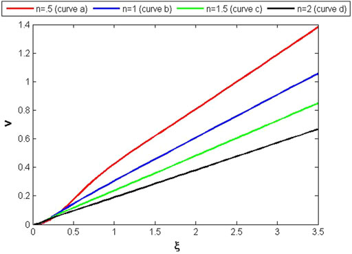
FIGURE 1. v(ξ) curves.

FIGURE 2

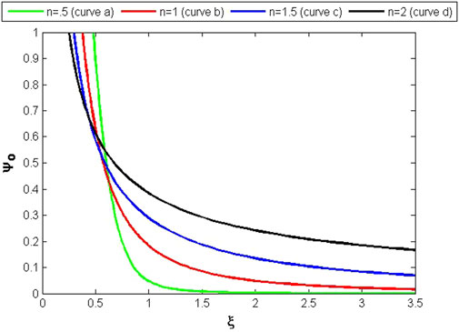
FIGURE 2. ψ_o(ξ) curves.

FIGURE 3

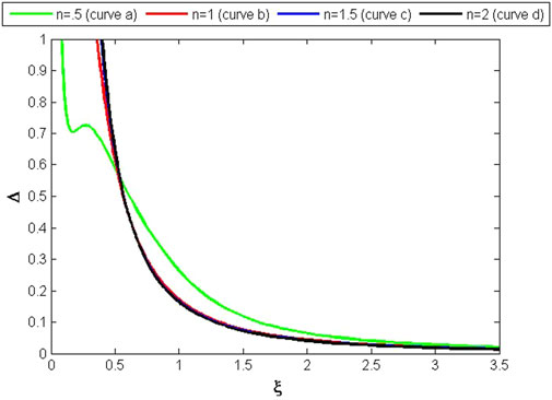
FIGURE 3. Δ(ξ) curves.

7.2 Case no. 2

CF in this case will be expressed as

$4\pi {\xi }^2\left(2\xi {\mathrm{\Delta }}^{\prime }+6\mathrm{\Delta }-{\mu }_{c}n\xi {\psi }^{n-1}{\psi }^{\prime }\right)=0,(84)$

for both α1 = .5 and α = .5, Figures 4–6 illustrate how v, ψ, and Δ behave for various n values. The system of ordinary DEs (61, 73, 71) is solved to achieve these characteristics numerically.

FIGURE 4

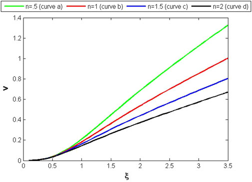
FIGURE 4. v(ξ) curves.

FIGURE 5

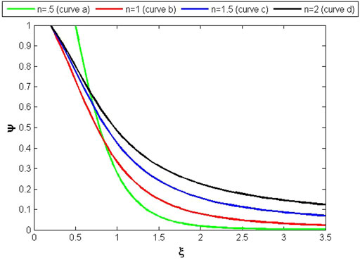
FIGURE 5. ψ(ξ) curves.

FIGURE 6

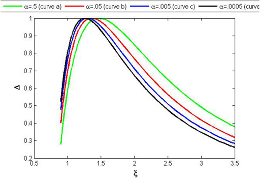
FIGURE 6. Δ(ξ) curves.

Vanishing CF Y_TF = 0 with class I GPs (γ = 1) will be regarded as

$4\pi {\xi }^2\left(2\xi {\mathrm{\Delta }}^{\prime }+6\mathrm{\Delta }-{\mu }_c\left(\xi e^{\psi }{\psi }^{\prime }+6\sinh \left(\psi \right)\right)\right).(85)$

The variables that are used in case 2(γ ≠ 1) constitute a set of first-order DEs (62, 77, 85). This set of DEs was also numerically solved for different values of parameters. Graphs of Figures 4–6 are used to illustrate the actions of v, ψ, and Δ.

8 Summary

Dark energy and dark matter are vital aspects of the universe which are explained by the GPEoS. It describes different scenarios of these two special features of astrophysics and gives information about the early and late universe (Babichev et al., 2004; Mukhopadhyay et al., 2008; Chavanis, 2012; Chavanis, 2014a; Chavanis, 2014b). Different self-gravitating system have been discussed through LEe over a long period of time (Lane, 1870; Chandrasekhar, 1939). The significance of this equation is that it helps to study the gravitational collapse of systems, stability of relativistic stellar objects, and density and pressure profiles of dark matter (Abellan et al., 2019; Bhatti and Tariq, 2019; Wojnar, 2019). In recent years, the concepts of GPEoS (Azam et al., 2016; Azam and Mardan, 2017; Mardan et al., 2018; Khan et al., 2019; Mardan et al., 2019; Mardan et al., 2020a; Mardan et al., 2020b; Khan et al., 2021a; Khan et al., 2021b), complexity factor (Abbas and Nazar, 2018; Herrera, 2018; Sharif and Butt, 2018; Khan et al., 2019; Sharif and Butt, 2019; Khan et al., 2021a; Khan et al., 2021b), and the Karmarkar condition (Karmakar, 1948; Maurya et al., 2015; Singh and Pant, 2016; Singh et al., 2017; Ramos et al., 2021) have all been widely used to explain various physical aspects and characteristics of self-gravitating compact objects. These three theories about self-gravitating stellar structures have been combined in the current study to explore a few of their characteristics (v, ψ_o, ψ, and Δ) under isothermal and non-isothermal regimes. For this reason, a generalized framework is built to create a modified version of the class I spherical LEe. The class I spherical TOV equation is constructed using field equations. Structure scalars are generated by means of the curvature tensor, the Weyl tensor and mass function are built, and CF is defined using these scalars. Class I spherical generalized LEes are developed through GPEoS for two cases: 1) mass density and 2) energy density in both non-isothermal and isothermal regimes. These LEes give us class I spherical GPs to study some features of self-gravitating stellar structures. Additionally, the energy conditions for each case have been determined. Vanishing CF with three pairs of LEes (55, 70), (61,73), and (64,77) generate three sets of DEs. The numerical solutions to these sets of DEs are presented graphically.

The numerical solution of the set of DEs (55, 70, 83) of case (1) is explained by the curves in Figures 1–3. The value of v for different values of n has been shown in Figure 1, which shows that the value of v is zero at the center of the spherical self-gravitating object, and it increases for higher values of n along the increasing direction of radius. It can also be seen that this object is more compact for n = .5 (curvea), and its compactness decreases for higher values of n(curved). The curves in Figure 2 show the behavior of ψ_o, which has its highest value at the center and it steadily diminishes as the radius increases. For n = .5, it is zero at the boundary surface. The curves in Figures 1, 2 are all smooth and exhibit normal behavior for various parameter values. The curves of Figure 3 express the response of variable Δ. It can be observed that these curves exhibit the same pattern as shown by the curves of Figure 2, except curve (a) of variable Δ, which shows some abnormal behavior at n = .5.

In case (2), Figure 4 shows the pattern of the variable v for different values of ξ. It has zero value at the center and gradually increases with the increase of ξ, and it attains maximum value at the boundary surface for the maximum value of n.

Figure 5 explains the behavior of variable ψ for different values of n. It attains maximum values at the center, which continuously decrease toward the boundary. It can be observed from Figure 6 that the measure of anisotropy has smaller values at the center of a self-gravitating object, and it attains maximum values at the middle of the radius of the object. It then starts decreasing until it reaches the minimum again at the boundary of the object.

Figures 7–9 illustrate the results of variables v, ψ, and Δ through the solutions of the set of DEs (62, 77, 85), for the isothermal regime. Figure 7 shows the exponential increase in variable v from the center to the boundary as the value of α decreases. Meanwhile, variable ψ in Figure 8 shows an exponential decrease as α decreases. The variable Δ in Figure 9 exhibits some abnormal behavior for smaller values of α. It can be seen from Figure 9 that Δ has the maximum value at the center and has a very small value at the boundary (curvea), and with a decrease in the value of α, it has higher values at the boundary (curvebandc), while at α = .0005, Δ changes its orientation and becomes minimum at the center (curved).

FIGURE 7

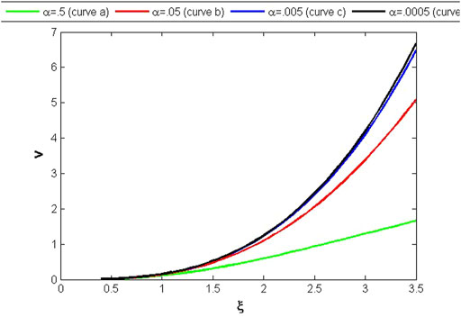
FIGURE 7. v(ξ) curves.

FIGURE 8

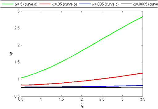
FIGURE 8. v(ξ) curves.

FIGURE 9

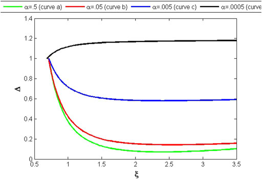
FIGURE 9. Δ(ξ) curves.

In the presence of anisotropic pressure, we have proposed the basic framework for the solutions of class I spherical generalized relativistic LEes with CF. We undertook this task by showing the perceptible presence of anisotropy in cosmological objects and its influence on the structure of such objects. Another factor is that fluid systems can be represented by the solutions of LEe with a number of applications in astrophysics and cosmology. The major goals of this study are to build a modified version of the class I spherical generalized LEe in relation to CF under isothermal and non-isothermal regimes and to numerically solve the systems of DEs. Some possible extensions to this work are the development of more generalized frameworks in modified theories of gravity such as f(R) and f(R, T) (Manzor and Shahid, 2021; Mumtaz et al., 2022).

Data availability statement

The original contributions presented in the study are included in the article/supplementary material, further inquiries can be directed to the corresponding authors.

Author contributions

All authors listed have made a substantial, direct, and intellectual contribution to the work and approved it for publication.

Funding

This work was financially supported by Zhejiang Normal University for Postdoctoral project (No. YS304023912).

Conflict of interest

The authors declare that the research was conducted in the absence of any commercial or financial relationships that could be construed as a potential conflict of interest.

Publisher’s note

All claims expressed in this article are solely those of the authors and do not necessarily represent those of their affiliated organizations, or those of the publisher, the editors, and the reviewers. Any product that may be evaluated in this article, or claim that may be made by its manufacturer, is not guaranteed or endorsed by the publisher.

References

Abbas, G., and Nazar, H. (2018). Complexity factor for anisotropic source in non-minimal coupling metric f(R) gravity. Eur. Phys. J. C78, 510.

CrossRef Full Text | Google Scholar

Abellan, G., Fuenmayor, E., Contreras, E., and Herrera, L. (2019). The general relativistic double polytrope for anisotropic matter. Phys. Dark Univ.30, 100632. doi:10.1016/j.dark.2020.100632

CrossRef Full Text | Google Scholar

Azam, M., and Mardan, S. A. (2017). Cracking of charged polytropes with generalized polytropic equation of state. Eur. Phys. J. C77, 113. doi:10.1140/epjc/s10052-017-4671-6

CrossRef Full Text | Google Scholar

Azam, M., Mardan, S. A., Noureen, I., and Rehman, M. A. (2016). Study of polytropes with generalized polytropic equation of state. Eur. Phys. J. C76, 315. doi:10.1140/epjc/s10052-016-4154-1

CrossRef Full Text | Google Scholar

Babichev, E., Dokuchaev, V., and Eroshenko, Y. (2004). Dark energy cosmology with generalized linear equation of state. Cl. Quant. Grav.22, 143–154. doi:10.1088/0264-9381/22/1/010

CrossRef Full Text | Google Scholar

Bel, L. (1961). Inductions électromagnétique et gravitationnelle. Ann. Inst. H. Poincaré17, 37.

Google Scholar

Bhatti, M. Z., and Tariq, Z. (2019). Conformally flat polytropes for anisotropic fluid in f (R) gravity. Eur. Phys. J Plus134, 521. doi:10.1140/epjp/i2019-12934-1

CrossRef Full Text | Google Scholar

Chandrasekhar, S. (1939). An introduction to the study of stellar structure. Chicago: University of Chicago.

Google Scholar

Chavanis, P. H. (2014). Models of universe with a polytropic equation of state: II. The late universe. Eur. Phys. J Plus129, 222. doi:10.1140/epjp/i2014-14222-0

CrossRef Full Text | Google Scholar

Chavanis, P. H. (2014). Models of universe with a polytropic equation of state: I. The early universe. Eur. Phys. J Plus129, 38. doi:10.1140/epjp/i2014-14038-x

CrossRef Full Text | Google Scholar

Chavanis, P. H. (2012). Partially relativistic self-gravitating Bose-Einstein condensates with a stiff equation of state. Astro. and Astrophy.127, 537.

Google Scholar

Eiesland, J. (1925). The group of motions of an Einstein space. Trans. Am. Math. Soc.27, 213–245. doi:10.1090/s0002-9947-1925-1501308-7

CrossRef Full Text | Google Scholar

Hendry, A. W. (1993). A polytropic model of the Sun. Am. J. Phys.61, 906–910. doi:10.1119/1.17362

CrossRef Full Text | Google Scholar

Herrera, L., and Barreto, W. (2004). Evolution of relativistic polytropes in the post–quasi–static regime. Gen. Rel. Grav.36, 127–150. doi:10.1023/b:gerg.0000006698.19527.4d

CrossRef Full Text | Google Scholar

Herrera, L., and Barreto, W. (2013). General relativistic polytropes for anisotropic matter: The general formalism and applications. Phys. Rev. D88, 084022. doi:10.1103/physrevd.88.084022

CrossRef Full Text | Google Scholar

Herrera, L., and Barreto, W. (2013). Newtonian polytropes for anisotropic matter: General framework and applications. Phys. Rev. D87, 087303. doi:10.1103/physrevd.87.087303

CrossRef Full Text | Google Scholar

Herrera, L., Di Prisco, A., Barreto, W., and Ospino, J. (2014). Conformally flat polytropes for anisotropic matter. Gen. Relat. Gravit.46, 1827. doi:10.1007/s10714-014-1827-7

CrossRef Full Text | Google Scholar

Herrera, L., Di Prisco, A., and Ibanez, J. (2011). Role of electric charge and cosmological constant in structure scalars. Phys. Rev. D84, 107501. doi:10.1103/physrevd.84.107501

CrossRef Full Text | Google Scholar

Herrera, L., Fuenmayor, E., and Leon, P. (2016). Cracking of general relativistic anisotropic polytropes. Phys. Rev. D93, 024047. doi:10.1103/physrevd.93.024047

CrossRef Full Text | Google Scholar

Herrera, L. (2018). New definition of complexity for self-gravitating fluid distributions: The spherically symmetric, static case. Phys. Rev. D.97, 044010.

CrossRef Full Text | Google Scholar

Herrera, L., Ospino, J., Di Prisco, A., Fuenmayor, E., and Troconis, O. (2009). Structure and evolution of self-gravitating objects and the orthogonal splitting of the Riemann tensor. Phys. Rev. D79, 064025.

CrossRef Full Text | Google Scholar

Horedt, G. P. (1973). Astron. Astrophys.23, 303.

Horedt, G. P. (1987). Physical characteristics ofN-dimensional, radially-symmetric polytropes. Astrophys. Space Sci.133, 81–106. doi:10.1007/bf00637425

CrossRef Full Text | Google Scholar

Kaplan, S. A., and Lupanov, G. A. (1965). The relativistic instability of polytropic spheres. Soviet Astron9, 233.

Google Scholar

Karmakar, K. R. (1948). Gravitational metrics of spherical symmetry and class one. Proc. Indian Acad. Sci.27, 56.

Google Scholar

Kaufmann, W. J. (1967). Polytropic spheres in general relativity. Astrophys. J.72, 754. doi:10.1086/110304

CrossRef Full Text | Google Scholar

Khan, S., Mardan, S. A., and Rehman, M. A. (2019). Framework for generalized polytropes with complexity factor. Eur. Phys. J. C1037, 1037. doi:10.1140/epjc/s10052-019-7569-7

CrossRef Full Text | Google Scholar

Khan, S., Mardan, S. A., and Rehman, M. A. (2021). Study of charged generalized polytropes with complexity factor. Eur. Phys. J. Plus136, 404. doi:10.1140/epjp/s13360-021-01395-y

CrossRef Full Text | Google Scholar

Khan, S., Mardan, S. A., and Rehman, M. A. (2021). Study of generalized cylindrical polytropes with complexity factor. Eur. Phys. J. C81, 831. doi:10.1140/epjc/s10052-021-09621-8

CrossRef Full Text | Google Scholar

Kovetz, A. (1968). Slowly rotating polytropes. Astrophys. J.154, 999. doi:10.1086/149820

CrossRef Full Text | Google Scholar

Lane, J. H. (1870). On the theoretical temperature of the Sun, under the hypothesis of a gaseous mass maintaining its volume by its internal heat, and depending on the laws of gases as known to terrestrial experiment. Am. J. Sci. Arts.50, 54–74. doi:10.2475/ajs.s2-50.148.57

CrossRef Full Text | Google Scholar

Malik, A., Ahmad, I., and Kiran, M. (2022). A study of anisotropic compact stars in f(R,ϕ,X)theory of gravity. Int. J. Geom. Methods Mod.19, 2250028. doi:10.1142/S0219887822500281

CrossRef Full Text | Google Scholar

Malik, A., Ahmad, M., Al Alwan, B., and Naeem, Z. (2022). Bardeen compact stars in modified f(G) gravity. Can. J. Phys.1, 452–462. doi:10.1139/cjp-2021-0411

CrossRef Full Text | Google Scholar

Malik, A. (2022). Analysis of charged compact stars in modified f(R,ϕ) theory of gravity. New Astron93, 101765. doi:10.1016/j.newast.2022.101765

CrossRef Full Text | Google Scholar

Malik, A., Ashraf, A., Naqvi, U., and Zhang, Z. (2022). Anisotropic spheres via embedding approach in f(R) gravity. Int. J. Geom. Methods Mod.19, 2250073. doi:10.1142/S0219887822500736

CrossRef Full Text | Google Scholar

Malik, A., Mofarreh, F., Ali, A., and Hamid, M. R. (2022). A study of charged stellar structure in modified f(R,ϕ,χ) gravity. Int. J. Geom. Methods Mod.19, 2250180. doi:10.1142/S0219887822501808

CrossRef Full Text | Google Scholar

Malik, A., Yousaf, Z., Jan, M., Shahzad, M. R., and Akram, Z. (2023). Analysis of charged compact stars in f(R,T) gravity using Bardeen geometry. Int. J. Geom. Methods Mod.20, 2350061. doi:10.1142/S0219887823500615

CrossRef Full Text | Google Scholar

Managhan, J. J., and Roxburgh, W. (1965). The structure of rapidly rotating polytropes. Mon. Not. R. astr.Soc.131, 13.

Google Scholar

Manzor, R., and Shahid, W. (2021). Evolution of cluster of stars in f(R) gravity. Phys. Dark Univ.33, 100544.

Google Scholar

Mardan, S. A., Asif, A., and Noureen, I. (2019). New classes of generalized anisotropic polytropes pertaining radiation density. Eur. Phys. J. Plus134, 242. doi:10.1140/epjp/i2019-12641-y

CrossRef Full Text | Google Scholar

Mardan, S. A., Noureen, I., Azam, M., Rehman, M. A., and Hussan, M. (2018). New classes of anisotropic models with generalized polytropic equation of state. Eur. Phys. J. C78, 516. doi:10.1140/epjc/s10052-018-5992-9

CrossRef Full Text | Google Scholar

Mardan, S. A., Rehman, M., Noureen, I., and Jamil, R. N. (2020). Impact of generalized polytropic equation of state on charged anisotropic polytropes. Eur. Phys. J. C80, 119. doi:10.1140/epjc/s10052-020-7647-x

CrossRef Full Text | Google Scholar

Mardan, S. A., Siddiqui, A. A., Noureen, I., and Jamil, R. N. (2020). New models of charged anisotropic polytropes with radiation density. Eur. Phys. J. Plus135, 3. doi:10.1140/epjp/s13360-019-00077-0

CrossRef Full Text | Google Scholar

Maurya, S. K., Gupta, Y. K., Ray, S., and Chowdhury, S. R. (2015). Spherically symmetric charged compact stars. Eur. Phys. J. C75, 389. doi:10.1140/epjc/s10052-015-3615-2

CrossRef Full Text | Google Scholar

Mukhopadhyay, U., Ray, S., and Dutta Choudhury, S. B. (2008). Dark energy with polytropic equation-of. Mod. phys. Lett. A23, 37.

CrossRef Full Text | Google Scholar

Mumtaz, S., Manzoor, R., Saqlain, M., and Ikram, A. (2022). Dissipative charged homologous model for cluster of stars in f(R,T) gravity. Phys. Dark Univ.37, 101096. doi:10.1016/j.dark.2022.101096

CrossRef Full Text | Google Scholar

Occhionero, F. (1967). Rotationally distorted polytropes second order approximation, n >= 2. Mem. Soc. Astron. Ital.38, 331.

Google Scholar

Pandey, S. C., Durgapal, M. C., and Pande, A. K. (1991). Relativistic polytropic spheres in general relativity. Astrophys. Space Sci.180, 75–92. doi:10.1007/bf00644230

CrossRef Full Text | Google Scholar

Pandey, S. N., and Sharma, S. P. (1982). Insufficiency of Karmarkar's condition. Gen. Relativ. Gravit.14, 113–115. doi:10.1007/bf00756917

CrossRef Full Text | Google Scholar

Ramos, A., Arias, C., Fuenmayor, E., and Contreras, E. (2021). Class I polytropes for anisotropic matter. Eur. Phys. J. C81, 203.

CrossRef Full Text | Google Scholar

Schlafli, L. (1871). Nota alla Memoria del sig. Beltrami, « Sugli spazii di curvatura costante ». Annali di Matematica Pura ed Applicata5, 170.

Google Scholar

Shamir, M. F. (2022). Relativistic krori-barua compact stars in f(R,T) gravity. Fortschr. Phys.70, 2200134. doi:10.1002/prop.202200134

CrossRef Full Text | Google Scholar

Sharif, M., and Butt, I. I. (2018). Complexity factor for static cylindrical system. Eur. Phys. J. C78, 850. doi:10.1140/epjc/s10052-018-6330-y

CrossRef Full Text | Google Scholar

Sharif, M., and Butt, I. I. (2019). Electromagnetic effects on complexity factor for static cylindrical system. Chin. J. Phys.61, 238–247. doi:10.1016/j.cjph.2019.07.009

CrossRef Full Text | Google Scholar

Sharma, J. P. (1981). Relativistic spherical polytropes: An analytical approach. Gen. Relat. Gravit.13, 663–667. doi:10.1007/bf00759409

CrossRef Full Text | Google Scholar

Singh, K. N., and Pant, N. (2016). A family of well-behaved Karmarkar spacetimes describing interior of relativistic stars. Eur. Phys. J. C76, 524. doi:10.1140/epjc/s10052-016-4364-6

CrossRef Full Text | Google Scholar

Singh, K. S., Pant, N., and Govender, M. (2017). Anisotropic compact stars in Karmarkar spacetime. Chi. Phys. C41, 015103. doi:10.1088/1674-1137/41/1/015103

CrossRef Full Text | Google Scholar

Singh, M., and Singh, G. (1983). The structure of the tidally and rotationally distorted polytropes. Astrophys. Space Sci.96, 313–319. doi:10.1007/bf00651675

CrossRef Full Text | Google Scholar

Tooper, R. F. (1965). Adiabatic fluid spheres in general relativity. Astrophys. J.142, 1541. doi:10.1086/148435

CrossRef Full Text | Google Scholar

Tooper, R. F. (1964). General relativistic polytropic fluid spheres. Astrophys. J.140, 434. doi:10.1086/147939

CrossRef Full Text | Google Scholar

Wojnar, A. (2019). Polytropic stars in Palatini gravity. Eur. Phys. J. C79, 51. doi:10.1140/epjc/s10052-019-6555-4

CrossRef Full Text | Google Scholar