 Fatemeh Bagheri
 Ramon E. Lopez
- Physics Department, University of Texas at Arlington, Arlington, TX, United States
Intense currents produced during geomagnetic storms dissipate energy in the ionosphere through Joule heating. This dissipation has significant space weather effects, and thus it is important to determine the ability of physics-based simulations to replicate real events quantitatively. Several empirical models estimate Joule heating based on ionospheric currents using the AE index. In this study, we select 11 magnetic storm simulations from the CCMC database and compare the integrated Joule heating in the simulations with the results of empirical models. We also use the SWMF global magnetohydrodynamic simulations for 12 storms to reproduce the correlation between the simulated AE index and simulated Joule heating. We find that the scale factors in the empirical models are half what is predicted by the SWMF simulations.
1 Introduction
Dayside merging and nightside reconnection produce plasma flow in the ionosphere, which can be intense and steady during a geomagnetic storm. The flow means that there is an electric field in Earth’s reference frame, and this electric field drives auroral electrojet currents that close the Birkeland currents driven by reconnection. This current dissipates energy in the ionosphere through frictional heating, which is generally referred to as Joule heating, although actual electromagnetic Joule heating should be calculated in the plasma frame (Vasyliūnas and Song, 2005). The energy dissipated through the Joule heating process is the second most important energy sink after the ring current (Akasofu, 1981) or even sometimes the most important (Harel et al., 1981; Lu et al., 1998). Thermospheric responses to Joule heating during magnetic storms can be quite significant (Deng et al., 2018). The ionospheric Joule dissipation heats the ionosphere and thermosphere so they can expand upward. These upward expansions can produce increased ionospheric ion outflow and satellite drag. The effect of satellite drag and the changes in the drag produced by space weather is an important effect that needs to be quantified (Doornbos and Klinkrad, 2006). Thus it is essential to understand how well the Joule heating produced by physics-based global simulations of magnetic storms compares to empirical estimates based on observations if such physics-based simulations are to be used for space weather prediction.
Studies often use empirical models of electric fields and conductivities to estimate Joule heating. These models typically do not represent the variability of electric fields, currents, and conductivities about the average. The contribution of electric-field variance to total Joule heating and its thermosphere/ionosphere effects can be substantial (Richmond, 2021). Therefore, to understand the energy transfer during geomagnetic storms and the coupling mechanism between the solar wind and the thermosphere-ionosphere-magnetosphere system, it is necessary to estimate the Joule heating rate accurately (Richmond and Lu, 2000).
Dissipation of energy through Joule heating is due to the current parallel to the electric field
where σP is the Pedersen conductivity, U is the neutral winds, and B is the magnetic field. Calculating the Joule heating rate requires Pedersen conductivity and electric field measurements over the entire polar region. However, there is still a challenge to monitor these quantities continuously over the entire high-latitude region. Ionospheric electric fields and conductivities could be directly measured locally by using rocket-borne instrumentation or more widely with incoherent scatter radar. Therefore several empirical models have been developed using geomagnetic indices such as Kp, AE, or AL to estimate the first approximation measure of the global Joule heating rates (Ahn et al., 1983; Foster et al., 1983; Baumjohann and Kamide, 1984). For example, Baumjohann and Kamide (1984) assumed that the height-integrated ionospheric conductivity simulates substorm activity in the AE index (Spiro et al., 1982; Zhou et al., 2011). However, these empirical models usually use small data sets and are based on assumptions that may not always be valid. For instance, Baumjohann and Kamide (1984) used the inversion method discussed by (Kamide et al., 1981), however, that technique may not always yield the best results and reflect the actual ionospheric electric fields and currents, a fact that was noted by the authors themselves. The empirical model of Weimer (2005) also solves for the ionospheric potential but uses a much larger database for its solution. However, for the purposes of this paper, we will use simple AE-based empirical formulations. This will allow us to determine if the global simulated Joule heating is related to the simulated AE in a manner similar to the empirical relationship between the Joule heating calculated from observation and the observed AE.
To estimate the energy dissipated through the Joule heating process, one can use global Magneto-Hydro-Dynamic (MHD) simulations. Such models have been used for many years to simulate storms and substorms and investigate the transfer of energy in the geospace system (e.g., Lopez et al., 1998; 2011). Palmroth et al. (2004) used the global MHD simulation code GUMICS-4 and found that the temporal variation of the Joule heating during substorms is well correlated with a commonly used AE-based empirical model, whereas, during the storm period, the simulated Joule heating was different from the empirical model. Following that study, in this paper, we use the Space Weather Modeling Framework (SWMF) MHD simulation for 12 storm events that had already been simulated with the results available at the Community Coordinated Modeling Center (CCMC) to compare the Joule heating resulting from simulations with empirical models. The SWMF simulation combines numerical models of the Inner Heliosphere, Solar Energetic Particles, Global Magnetosphere, Inner Magnetosphere, Radiation Belt, Ionosphere, and Upper Atmosphere into a parallel, high-performance model (Tóth et al., 2005). Two versions of the SWMF model are used on CCMC. All simulations selected in this paper are the version of v20180525.
2 Correlations between SWMF simulations and observations, using the SME index
In this section, we compare three empirical models of Joule heating with the output of SMWF simulation. We select 11 magnetic storms with Dst* ≤ −50 nT for the period between 2010 and 2020 from the storm sample provided in (Bagheri and Lopez, 2022). The information on the SWMF simulations of these storms at the CCMC is listed in Table 1 (for more information, see Supplementary Appendix A). We calculate the Joule heating using three empirical formulas that relate the Joule heating to the AE index:
• Model 1: UJH (GW) = 0.32AE (Baumjohann and Kamide, 1984),
• Model 2: UJH (GW) = 0.28AE + 0.9 (Østgaard et al., 2002a; b),
• Model 3: UJH (GW) = 0.23AE (Kalafatoglu Eyiguler et al., 2018).
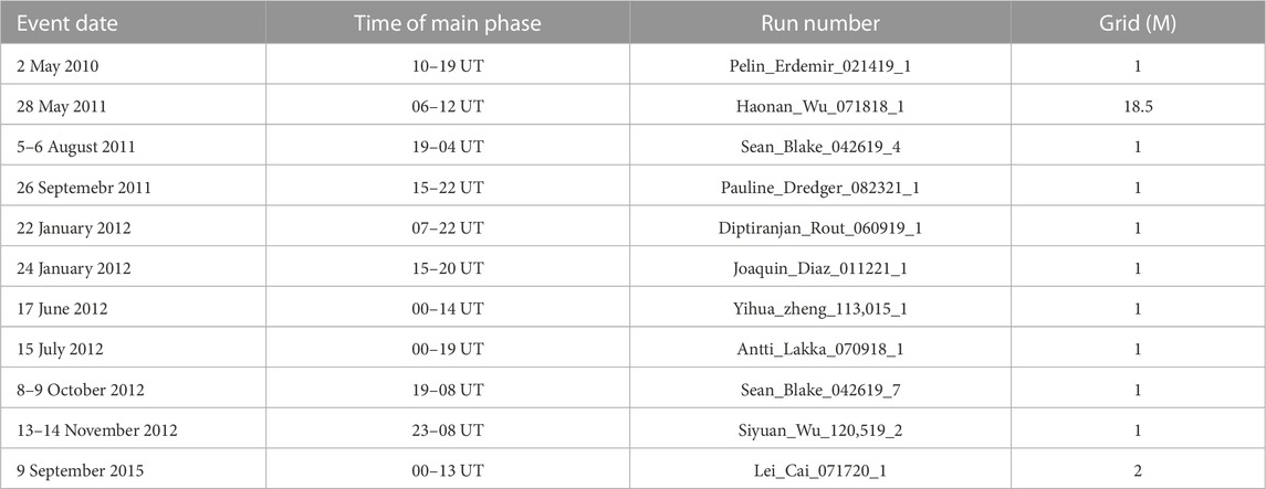
TABLE 1. Information on SWMF simulations on CCMC used to compare the simulated Joule heating and three empirical models. All selected simulations are real storm events and the version of v20180525.
The AE index (Nose et al., 2015) is produced at a 1-min cadence using data from up to 12 magnetometer stations at latitudes that correspond to the average location of the auroral oval. SuperMAG now produces SME, an equivalent to AE, at a 1-min cadence (Gjerloev, 2012). SME is the difference between upper (SMU) and lower (SML) indices. SMU and SML are based on the H-component measured at stations in the latitudes of the auroral oval, with baseline removal carried out. The difference between AE and SME is the number of stations used in their derivation. While AE uses (at maximum) 12 stations, the number of stations used to derive SME is roughly an order of magnitude larger and the stations cover a broader range of latitude. Using the 1-min SME data from SuperMag in Eq. 2 instead of AE, we can better estimate the energy dissipated through Joule heating for each storm since the SME index has better coverage than AE, particularly at lower latitudes where intense electrojets can be found during magnetic storms because of the expanded polar cap. Furthermore, we use data from Active Magnetosphere and Planetary Electrodynamics Response Experiment (AMPERE) to measure the strength of Birkeland (Field-Aligned Currents (FACs)) current during each storm. AMPERE produces global maps of the Birkeland current using magnetometer data from over 70 satellites in the Iridium network with a cadence of 2 min (Anderson et al., 2000).
We compare the solar wind input for the simulations to the 1-min OMNI data provided by CDAWeb for each event. We only use the simulations whose inputs are in perfect agreement with OMNI data. Figure 1 illustrates two examples of storms where the solar wind data from OMNI is the same as the simulation input. This is not the case for some storms in the CCMC database, and there can be a substantial difference between the input for the simulations and the actual OMNI data during the event.
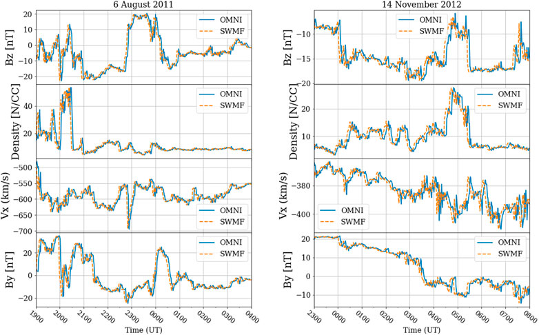
FIGURE 1. Left: the solar wind data from OMNI and SWMF input for the magnetic storm on 6 August 2011. The simulation input and OMNI data are highly correlated with a correlation coefficient of 0.99 with a lagtime of 4 min. Right: the solar wind data from OMNI and SWMF input for the magnetic storm on 14 November 2012. The simulation input and OMNI data are highly correlated with a correlation coefficient of 0.99 with a lagtime of 6 min.
We find that good agreement of the simulation input with the OMNI data does not necessarily result in a good correlation between empirical and SWMF Joule heating. For instance, although in both cases shown in Figure 1, the inputs of SWMF simulations of the storms are consistent with the OMNI data, in the first event (6 August 2011), the resulting Joule heating is highly correlated with all the three empirical models, whereas in the second event (14 November 2012) they are not (Figure 2). The lagtime between OMNI data and SWMF inputs in Figures 1, 2 is because OMNI data report the value of the solar wind parameters as they projected at the Bow shock region, while SMWF input data are projected at 32 RE.
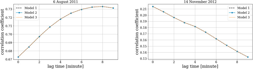
FIGURE 2. The correlation coefficient of Joule heating resulted from three empirical models and SWMF simulations as a function of lagtime during the main phase of left: the storm happened on 6 August 2011, and, right: the storm happened on 14 November 2012.
We calculate the Pearson correlation coefficient between each empirical model of Joule heating and SWMF-simulated Joule heating for all storms. Moreover, since each storm has a different duration (i.e., different sample size), we calculated the standard error for Pearson correlation using Fisher’s r-to-z transformation method, which results in asymmetrical confidence intervals. Furthermore, for each storm, we find the best linear fit of the simulated Joule heating as a function of Joule heating from empirical models. We summarize our results in Table 2. All three empirical models have the same Pearson correlation coefficient up to 5 decimal digits. However, Model 2: UJH (GW) = 0.28AE + 0.9 [(Østgaard et al., 2002a; b)] has the greatest slopes in all events, and thus it fits better to the simulations.
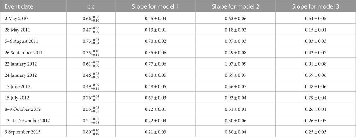
TABLE 2. Correlation coefficients between the simulated Joule heating and Joule heating from empirical models. All three empirical models have the same correlation coefficient of up to 5 decimals. Moreover, the slopes of the best linear fits of the simulated Joule heating as a function of Joule heating from empirical models are reported in columns 3–5.
Additionally, we investigate the Pearson correlation between the AMPERE Birkeland current and the Birkeland current in the simulations. Similar to the previous Joule heating calculations, we calculated the standard error for Pearson correlation using Fisher’s r-to-z transformation method. We also find the best linear fits of simulated and the AMPERE Birkeland currents. As represented in Table 3, SWMF simulations predict a smaller amount of Birkeland currents for all events in this study, approximately by a factor of 1/3 for the events with c. c ≥ 0.8.
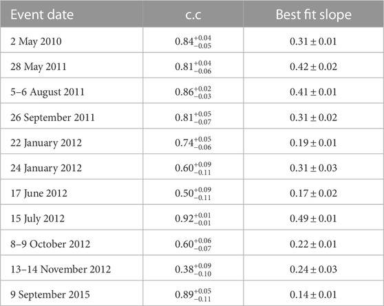
TABLE 3. Correlation coefficients and the slopes of best linear fits of the simulated FAC and AMPERE data.
As represented in Figure 3 we find that the correlation coefficient between Joule heatings (simulated and empirical) increases as the correlation coefficient of Birkeland currents (simulated and observed by AMPERE) increases. This result corroborates results in (Robinson et al., 2021). They showed the SME index could be accurately deduced from AMPERE data with a correlation coefficient of 0.84. In other words, if SWMF simulation predicts the Birkeland currents correctly, then the Joule heating would be simulated consistently with observations. This is not surprising for two reasons. First, in the simulation results, agreeing with the observed Birkeland current intensity, one can have confidence that the simulation accurately represented the solar wind-magnetosphere interaction and that other simulation features would also bear a reasonable resemblance to reality. Moreover, since the auroral electrojets are the ionospheric closure currents for the Birkeland currents (as represented by the correlation between the simulated SME and simulated Birkeland current), getting the Birkeland currents right will mean that the SME will also be (more or less) correct, at least in terms of the variations if not the absolute magnitude. This result can be used to identify periods when the real-time SMWF simulation of Joule heating is accurate during the geomagnetic storms by calculating a running correlation between the SWMF results and Birkeland current observations.
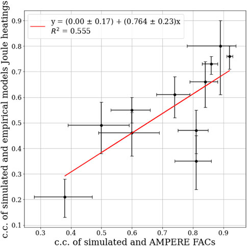
FIGURE 3. Pearson correlation coefficient between the empirical and simulated Joule heating as a function of the correlation coefficient between the empirical and simulated Birkeland currents for the storms in our sample. All the standard errors for Pearson correlation were calculated by using Fisher’s r-to-z transformation method.
3 Correlations between AE and joule heating using SWMF simulations
To investigate the relationship between Joule heating and the AE index, we use the simulations of 12 magnetic storms (Bagheri and Lopez, 2022) with Dst* ≤ −50 nT. Table 4 summarizes the information on these events. For each storm, we find the best linear fit between simulated Joule heating and the simulated AE index. All these linear fits are shown in Figure 4.
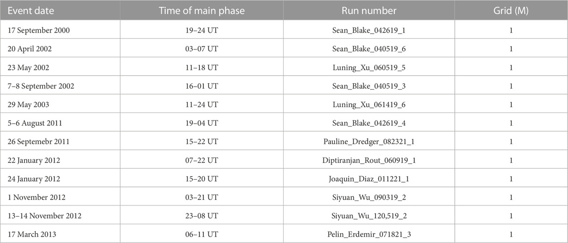
TABLE 4. Information on the SWMF simulations on CCMC used to study the relationship between simulated JH and the AE index. All simulations are real event simulations. For more information see Supplementary Appendix A.
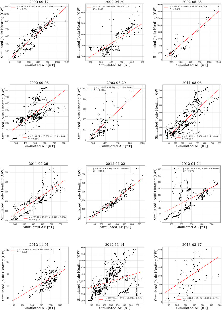
FIGURE 4. Simulated Joule heating as a function of simulated AE index for the events in Table 4.
Taking the average of all the storms’ linear fits between the simulated Joule heating as a function of the simulated AE index, we can write
Comparing this result to empirical models, one can conclude that the SWMF model predicts a greater dependency on the AE index for the Joule heating than the empirical models considered in the paper.
4 Conclusion and discussion
In this paper, we compare the empirical models of the Joule heating with the results of SWMF simulations for a set of storm events already simulated and available at the CCMC website. We find that the SWMF simulations predict a smaller amount of Joule heating compared to empirical estimates using the SME index. Moreover, we find that events with a good correlation between the simulated ionospheric current and the AMPERE currents show a higher correlation between the simulated Joule heating and the empirical model.
The SWMF simulation uses the Ridley conductance model (Ridley et al., 2004). This model has two major sources of ionospheric conductance: solar EUV conductance on the dayside and auroral precipitative conductance in the polar regions. Other sources of conductance, such as seasonal dependencies, are added as functions of the dominant sources of conductance, solar zenith angle, or scalar constants (Mukhopadhyay et al., 2020). This model produces broad regions of locally elevated conductance that are discontinuous between regions of strong FACs. On the other, the overall conductance can be lower because of unrealistically low values of particle precipitation (Wiltberger et al., 2012). Therefore, during extreme events, it leads to possible unrealistic values of global quantities such as cross polar cap potential or FACs (Mukhopadhyay et al., 2022; Anderson et al., 2017; Liemohn et al., 2018; Welling et al., 2018; , 2022). Consistent with these studies we find that SWMF simulations underpredict Birkeland currents for all storm events in this study.
To calculate Joule heating using empirical equations, we used the SME index instead of the AE index. The SME index used significantly more stations than the AE index, especially in lower latitudes. However, the Ridley model domain in the SWMF simulation is considerably limited, from the magnetic pole to the magnetic latitude of 60°C for all magnetic local times (MLTs). This could lead to inconsistency between the prediction of the SWMF simulations and empirical models for Joule heating.
Two storm cases in Section 2 (13–14 November 2012 and 26 September 2011) show low correlation between the SWMF simulated Joule heating and the empirical models. To see what physical parameters are involved in the correlation coefficients, we investigated the dependency of the correlation coefficients with the solar wind parameters such as velocity, Mach number, and IMF during the main phase of the storms. Our result showed that there is not any significant evidence that these parameters can affect the correlation between SWMF and empirical models. However, increasing the magnitude of the IMF (averaged over the main phase of the storms) decreases the correlation, so there is a weak dependency on the IMF magnitude (with R2 = 0.26). This result is consistent with the conclusion of (Welling et al., 2018), which shows that during intense events, the ionospheric model in the SWMF simulation (Ridley et al., 2004) does not predict the ionospheric conductance and indices accurately.
Furthermore, we investigate the relationship between the simulated Joule heating and the simulated AE index. We find that the scale factor between the AE index and the amount of Joule heating is about two times greater than in the empirical models. One possible reason for the inconsistency is that the SWMF model does not predict the AE index well (Haiducek et al., 2017; Kitamura et al., 2008). The SWMF Biot-Savart calculation of the ground magnetic perturbation due to ionospheric currents does not include magnetotelluric effects. Moreover, the simulation grid latitudinal resolution is 1°–2° (100 km–200 km), spreading out the currents compared to reality. These effects could easily result in a factor of 2 in the calculated ground perturbation compared to observations, even if the total simulated Joule heating and current in the ionosphere is actually similar to reality.
The inconsistency between simulation results and empirical models is not limited to the SWMF simulation. Wiltberger et al. (2012) examine the Coupled Magnetosphere Ionosphere Thermosphere (CMIT) model. In CMIT, the magnetosphere model is the Lyon–Fedder–Mobarry (LFM) global magnetospheric simulation (Lyon et al., 2004). They found a considerable disagreement between the simulation and observational data in predicting the Cross Polar Cap Potential (CPCP) strength, hemispheric power, and SYMH index. In their study, CPCP is highly overestimated due to the weak electron precipitation power seen in the hemispheric power, leading to a low overall ionospheric conductance (Wiltberger et al., 2012). In addition, Pirnaris et al. (2023) compared the evolution of the globally-integrated Joule heating rates between the two Global Circulation Models (GCM) of the Earth’s upper atmosphere (the Global Ionosphere/Thermosphere Model (GITM) and the Thermosphere-Ionosphere-Electrodynamics General Circulation Model (TIE-GCM)) with the several empirical models during the storm of 17 March 2015. They found that all empirical models, on average, underestimate Joule heating rates compared to both GITM and TIE-GCM, whereas TIE-GCM calculates lower heating rates compared to GITM.
In conclusion, there are still discrepancies between empirical models and global MHD simulations in predicting/estimating Joule heating. In this paper, we demonstrate this gap in the understanding and parametrization of Joule heating during storm times. In February 2022, 40 Space-X satellites were lost due to the enhanced Joule heating during a storm (Dang et al., 2022). Therefore, a real-time prediction of Joule heating is essential for predicting the possible atmospheric drag of the satellites. Our result shows that one can use SWMF simulations for real-time prediction of Joule heating during geomagnetic storms if the SWMF result of Birkeland current is highly correlated with observations.
Data availability statement
The original contributions presented in the study are included in the article/supplementary material, further inquiries can be directed to the corresponding author.
Author contributions
FB did this research as a Ph.D. student under the supervision of RL. All authors contributed to the article and approved the submitted version.
Acknowledgments
We gratefully acknowledge the SuperMAG website and the data provided by SuperMAG collaborators. The SME data can be found at https://supermag.jhuapl.edu/indices/ for the periods described in the paper. We thank the AMPERE team and the AMPERE Science Center for providing the Iridium-derived data products. The AMPERE Birkeland current data can be found at https://ampere.jhuapl.edu/products/itot/daily.html for each day at a 2-min time resolution. We acknowledge the use of the OMNI data set, which was obtained from CDAWeb using the Space Physics Data Facility (SPDF). We acknowledge the support of the US National Science Foundation (NSF) under Grant No. 1916604. We also gratefully acknowledge the Community Coordinated Modeling Center (CCMC) at Goddard Space Flight Center. Simulation results have been provided by the CCMC through their public Runs on Request system (http://ccmc.gsfc.nasa.gov). The CCMC is a multi-agency partnership between NASA, AFMC, AFOSR, AFRL, AFWA, NOAA, NSF, and ONR.
Conflict of interest
The authors declare that the research was conducted in the absence of any commercial or financial relationships that could be construed as a potential conflict of interest.
Supplementary material
The Supplementary Material for this article can be found online at: https://www.frontiersin.org/articles/10.3389/fspas.2023.1170390/full#supplementary-material
Publisher’s note
All claims expressed in this article are solely those of the authors and do not necessarily represent those of their affiliated organizations, or those of the publisher, the editors and the reviewers. Any product that may be evaluated in this article, or claim that may be made by its manufacturer, is not guaranteed or endorsed by the publisher.
References
Ahn, B.-H., Akasofu, S.-I., and Kamide, Y. (1983). The joule heat production rate and the particle energy injection rate as a function of the geomagnetic indices ae and al. J. Geophys. Res. Space Phys.88, 6275–6287. doi:10.1029/ja088ia08p06275
Akasofu, S.-I. (1981). Energy coupling between the solar wind and the magnetosphere. Space Sci. Rev.28, 121–190. doi:10.1007/bf00218810
Anderson, B. J., Korth, H., Welling, D. T., Merkin, V. G., Wiltberger, M. J., Raeder, J., et al. (2017). Comparison of predictive estimates of high-latitude electrodynamics with observations of global-scale birkeland currents. Space weather.15, 352–373. doi:10.1002/2016sw001529
Anderson, B. J., Takahashi, K., and Toth, B. A. (2000). Sensing global birkeland currents with iridium® engineering magnetometer data. Geophys. Res. Lett.27, 4045–4048. doi:10.1029/2000gl000094
Bagheri, F., and Lopez, R. E. (2022). Solar wind magnetosonic mach number as a control variable for energy dissipation during magnetic storms. Front. Astronomy Space Sci.9, 960535. doi:10.3389/fspas.2022.960535
Baumjohann, W., and Kamide, Y. (1984). Hemispherical joule heating and the ae indices. J. Geophys. Res. Space Phys.89, 383–388. doi:10.1029/ja089ia01p00383
Dang, T., Li, X., Luo, B., Li, R., Zhang, B., Pham, K., et al. (2022). Unveiling the space weather during the starlink satellites destruction event on 4 february 2022. Space weather.20, e2022SW003152. doi:10.1029/2022sw003152
Deng, Y., Sheng, C., Tsurutani, B. T., and Mannucci, A. J. (2018). Possible influence of extreme magnetic storms on the thermosphere in the high latitudes. Space weather.16, 802–813. doi:10.1029/2018sw001847
Doornbos, E., and Klinkrad, H. (2006). Modelling of space weather effects on satellite drag. Adv. Space Res.37, 1229–1239. doi:10.1016/j.asr.2005.04.097
Foster, J., St.-Maurice, J.-P., and Abreu, V. (1983). Joule heating at high latitudes. J. Geophys. Res. Space Phys.88, 4885–4897. doi:10.1029/ja088ia06p04885
Gjerloev, J. (2012). The supermag data processing technique. J. Geophys. Res. Space Phys.117. doi:10.1029/2012ja017683
Haiducek, J. D., Welling, D. T., Ganushkina, N. Y., Morley, S. K., and Ozturk, D. S. (2017). Swmf global magnetosphere simulations of january 2005: Geomagnetic indices and cross-polar cap potential. Space weather.15, 1567–1587. doi:10.1002/2017sw001695
Harel, M., Wolf, R., Reiff, P., Spiro, R., Burke, W., Rich, F., et al. (1981). Quantitative simulation of a magnetospheric substorm 1. model logic and overview. J. Geophys. Res. Space Phys.86, 2217–2241. doi:10.1029/ja086ia04p02217
Kalafatoglu Eyiguler, E., Kaymaz, Z., Frissell, N. A., Ruohoniemi, J., and Rastätter, L. (2018). Investigating upper atmospheric joule heating using cross-combination of data for two moderate substorm cases. Space weather.16, 987–1012. doi:10.1029/2018sw001956
Kamide, Y., Richmond, A., and Matsushita, S. (1981). Estimation of ionospheric electric fields, ionospheric currents, and field-aligned currents from ground magnetic records. J. Geophys. Res. Space Phys.86, 801–813. doi:10.1029/ja086ia02p00801
Kitamura, K., Shimazu, H., Fujita, S., Watari, S., Kunitake, M., Shinagawa, H., et al. (2008). Properties of ae indices derived from real-time global simulation and their implications for solar wind-magnetosphere coupling. J. Geophys. Res. Space Phys.113. doi:10.1029/2007ja012514
Liemohn, M. W., McCollough, J. P., Jordanova, V. K., Ngwira, C. M., Morley, S. K., Cid, C., et al. (2018). Model evaluation guidelines for geomagnetic index predictions. Space weather.16, 2079–2102. doi:10.1029/2018sw002067
Lopez, R. E., Merkin, V., and Lyon, J. (2011). The role of the bow shock in solar wind-magnetosphere coupling. Ann. Geophys. Copernic. GmbH)29, 1129–1135. doi:10.5194/angeo-29-1129-2011
Lopez, R., Goodrich, C., Wiltberger, M., Papadopoulos, K., and Lyon, J. (1998). Simulation of the march 9, 1995 substorm and initial comparison to data. Geophys. MONOGRAPH-AMERICAN Geophys. UNION104, 237–246.
Lu, G., Baker, D., McPherron, R., Farrugia, C. J., Lummerzheim, D., Ruohoniemi, J., et al. (1998). Global energy deposition during the january 1997 magnetic cloud event. J. Geophys. Res. Space Phys.103, 11685–11694. doi:10.1029/98ja00897
Lyon, J., Fedder, J., and Mobarry, C. (2004). The lyon–fedder–mobarry (lfm) global mhd magnetospheric simulation code. J. Atmos. Solar-Terrestrial Phys.66, 1333–1350. doi:10.1016/j.jastp.2004.03.020
Mukhopadhyay, A. (2022). Statistical comparison of magnetopause distances and cpcp estimation by global mhd models. Authorea Preprints.
Mukhopadhyay, A., Welling, D. T., Liemohn, M. W., Ridley, A. J., Chakraborty, S., and Anderson, B. J. (2020). Conductance model for extreme events: Impact of auroral conductance on space weather forecasts. Space weather.18, e2020SW002551. doi:10.1029/2020sw002551
Nose, M., Iyemori, T., Sugiura, M., and Kamei, T. (2015). Geomagnetic ae index. Kyoto: World Data Center for Geomagnetism. 10, 15–031.
Østgaard, N., Germany, G., Stadsnes, J., and Vondrak, R. (2002a). Energy analysis of substorms based on remote sensing techniques, solar wind measurements, and geomagnetic indices. J. Geophys. Res. Space Phys.107, 1233. SMP–9. doi:10.1029/2001ja002002
Østgaard, N., Vondrak, R., Gjerloev, J., and Germany, G. (2002b). A relation between the energy deposition by electron precipitation and geomagnetic indices during substorms. J. Geophys. Res. Space Phys.107, 1246. SMP–16. doi:10.1029/2001ja002003
Palmroth, M., Janhunen, P., Pulkkinen, T., and Koskinen, H. (2004). Ionospheric energy input as a function of solar wind parameters: Global mhd simulation results. Ann. Geophys. Copernic. GmbH)22, 549–566. doi:10.5194/angeo-22-549-2004
Pirnaris, P. I., Sarris, T. E., Tourgaidis, S., and Ridley, A. J. (2023). Comparison of global joule heating estimates in gitm, tie-gcm and empirical formulations during st. patrick’s day 2015 geomagnetic storm. Authorea Preprints.
Richmond, A. D. (2021). “Joule heating in the thermosphere,” in Upper atmosphere dynamics and energetics (New Jersey, United States: Wiley). 1–18.
Richmond, A., and Lu, G. (2000). Upper-atmospheric effects of magnetic storms: A brief tutorial. J. Atmos. Solar-Terrestrial Phys.62, 1115–1127. doi:10.1016/s1364-6826(00)00094-8
Ridley, A., Gombosi, T. I., and DeZeeuw, D. (2004). Ionospheric control of the magnetosphere: Conductance. Ann. Geophys. Copernic. GmbH)22, 567–584. doi:10.5194/angeo-22-567-2004
Robinson, R., Zanetti, L., Anderson, B., Vines, S., and Gjerloev, J. (2021). Determination of auroral electrodynamic parameters from ampere field-aligned current measurements. Space weather.19, e2020SW002677. doi:10.1029/2020sw002677
Spiro, R., Reiff, P. H., and Maher, L. (1982). Precipitating electron energy flux and auroral zone conductances-an empirical model. J. Geophys. Res. Space Phys.87, 8215–8227. doi:10.1029/ja087ia10p08215
Tóth, G., Sokolov, I. V., Gombosi, T. I., Chesney, D. R., Clauer, C. R., De Zeeuw, D. L., et al. (2005). Space weather modeling framework: A new tool for the space science community. J. Geophys. Res. Space Phys.110, A12226. doi:10.1029/2005ja011126
Vasyliūnas, V. M., and Song, P. (2005). Meaning of ionospheric joule heating. J. Geophys. Res. Space Phys.110, A02301. doi:10.1029/2004ja010615
Weimer, D. (2005). Improved ionospheric electrodynamic models and application to calculating joule heating rates. J. Geophys. Res. Space Phys.110, A05306. doi:10.1029/2004ja010884
Welling, D., Ngwira, C., Opgenoorth, H., Haiducek, J., Savani, N., Morley, S. K., et al. (2018). Recommendations for next-generation ground magnetic perturbation validation. Space weather.16, 1912–1920. doi:10.1029/2018sw002064
Wiltberger, M., Qian, L., Huang, C.-L., Wang, W., Lopez, R. E., Burns, A. G., et al. (2012). Cmit study of cr2060 and 2068 comparing l1 and mas solar wind drivers. J. Atmos. solar-terrestrial Phys.83, 39–50. doi:10.1016/j.jastp.2012.01.005
Keywords: ionospheric joule heating, CCMC simulations, SWMF simulations, AE index, FAC
Citation: Bagheri F and Lopez RE (2023) Comparison of empirical models of ionospheric heating to global simulations. Front. Astron. Space Sci. 10:1170390. doi: 10.3389/fspas.2023.1170390
Received: 20 February 2023; Accepted: 15 May 2023;
Published: 08 June 2023.
Edited by:
Libo Liu, Institute of Geology and Geophysics (CAS), ChinaReviewed by:
Xu Zhou, Chinese Academy of Sciences (CAS), ChinaTong Dang, University of Science and Technology of China, China
Copyright © 2023 Bagheri and Lopez. This is an open-access article distributed under the terms of the Creative Commons Attribution License (CC BY). The use, distribution or reproduction in other forums is permitted, provided the original author(s) and the copyright owner(s) are credited and that the original publication in this journal is cited, in accordance with accepted academic practice. No use, distribution or reproduction is permitted which does not comply with these terms.
*Correspondence: Fatemeh Bagheri, ZnhiMTQ5NUBtYXZzLnV0YS5lZHU=