Signature of Y-forking in ionogram traces observed at low-mid latitude Indian station, New Delhi, during the earthquake events of 2020: ionosonde observations

We have examined ionospheric response to eleven earthquake events measuring less than four on the Richter scale during the year 2020 that occurred in the vicinity of New Delhi (28.6°N, 77.2°E, 42.4°N dip). We have used ionogram traces, manually scaled critical ionospheric layer parameters using SAO explorer obtained from Digisonde along with the O(¹D) airglow observations from a multi-wavelength all-sky airglow imager installed at Hanle, Ladakh, India (32.7°N, 78.9°E, 24.1°N dip). Perceptible ionospheric perturbations 2–9 days prior to these earthquake events resulting in more than 250% variation in electron density are observed. We found distortion of ionogram trace in the form of Y forking majorly at New Delhi on the precursor day and after the earthquake event. Traces of Y forked ionograms were also observed at Ahmedabad (23°N, 72°E, 15°N dip) and Trivandrum (8.5°N, 76.9°E, 0.5°N dip). These Y-forked ionograms are one of the first observations during any earthquake events and are looked at as a signature of Travelling Ionospheric Disturbances (TIDs).

1 Introduction

Coupling between lithospheric and ionospheric variations is mainly associated with pre-earthquake ionospheric anomalies (PEIAs). PEIAs are considered earthquake precursors mainly based on lithosphere–atmosphere–ionosphere coupling (LAIC) models such as the rising of gases (specifically radon) and other particles from the seismogenic zone during the earthquake preparation period (Pulinets and Ouzounov, 2011) or activation of positive holes from the Earth’s crust, causing ionization of nearby atmospheres followed by abnormalities in the upper atmosphere (Freund, 2011; Freund, 2013). The seismo-ionospheric effects in the F-layer of the ionosphere have been extensively studied in the last two decades (Rishbeth, 2007; Liu et al., 2011; Maruyama and Shinagawa, 2014; Ouzounov et al., 2018; Pulinets et al., 2021; Xiong et al., 2021).

According to reports, the effects of an impending earthquake can be observed in the earthquake-prone region, spanning approximately 1,000 km in diameter, prior to the main shock (Dobrovolsky et al., 1979). These effects can manifest in the ionospheric F-region, leading to changes in electron density (either enhancement or reduction), critical frequency (f_oF₂), electron temperature, and total electron content (TEC) (Pulinets et al., 1994; Ryu et al., 2014; Zhu et al., 2021). The magnitude of these changes depends on various factors such as the earthquake’s depth, location, magnitude, and the distance between the epicenter and ionospheric monitoring station (Larkina et al., 1989; Pulinets, 2004; Liu et al., 2006; 2007; Le et al., 2011; Shah and Jin, 2015; Parrot et al., 2016; Gupta and Upadhayaya, 2017; De Santis et al., 2019; Ghamry et al., 2021).

Seismic waves originating from the epicenter during an earthquake event cause atmospheric pressure disturbances (Bolt, 1964; Blanc, 1985) when propagated upward to the bottom-side F layer (Artru et al., 2004; Chum et al., 2012; Jing et al., 2019; Pundhir et al., 2021), thereby modifying the ionospheric plasma density appreciably as there is more collision between neutral particles and ions.

Such co-seismic ionospheric disturbances before earthquakes are detected as changes in TEC (Astafyeva et al., 2009; Liu et al., 2010; Ouzounov et al., 2015; Gupta and Upadhayaya, 2017; Pundhir et al., 2021; Tariq et al., 2021). Ouzounov et al. (2015) investigated the global ionosphere maps (GIM-GPS/TEC) for the M7.8 and M7.3 April 2015 devastating Nepal earthquakes to indicate a close correlation between ionospheric anomalies and these earthquake events. The 6.9 magnitude 2018 Bayan earthquake has also been studied in detail for co-seismic and precursory phenomena (Piersanti et al., 2020) using CSES, ERA-5, and ground data. Shi et al. (2021) investigated ionospheric anomalies in the F₂ region (NmF₂), vertical structure (the GNSS radio occultation profile), and multi-height (electron density) pre-earthquake anomalies for the Concepción, Chile, earthquake (27 February 2010, Mw 8.8). Gupta and Upadhayaya (2017) had found perceptible ionospheric perturbations that indicate toward the possibility of seismo-ionospheric coupling. These perturbations appeared as enhancements and depressions in the (f_oF₂) critical frequency.

The ionospheric anomaly exhibits a characteristic of traveling ionospheric disturbances and is seen as a distortion of ionogram traces (Leonard and Barnes Jr., 1965; Yuen et al., 1969; Liu and Sun, 2011; Maruyama et al., 2011; 2012; Harris et al., 2012; Maruyama and Shinagawa, 2014; Pradipta et al., 2015). Such distortions are reported to appear in four shapes: Heisler (1958) examined these types of anomalies as (a) Type A or the “split” type anomaly identified as a distinct forking of the trace at F₂ penetration frequency, (b) Type B or the “Z” type anomaly has a “Z” letter type fold in the F₂ trace, (c) Type C or the “double peak” anomaly is seen as a cusp shape forming two distinct F₁ peaks, and (d) Type D or the “cusp” anomaly is seen as a cusp-shaped trace at the F₂ trace. Each of these anomalies is shown in Figure 1A. When a traveling plasma disturbance passes through the ionosphere, complex reflections from the curved isoionic surfaces cause Type A and Type B abnormalities. Type C anomaly occurs as a complexity in the F₁ layer, while Type D occurs in the F₂ layer due to non-vertical reflections. Splitting of the ionogram near the F₂ layer in the shape of Y-forking (Type A) is a distortion reported to be seen during earthquake events. A sample of a normal ionogram along with an ionogram exhibiting such Y-forking is shown in Figure 1B.

FIGURE 1

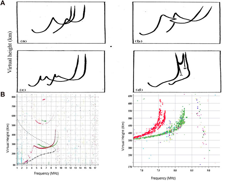
FIGURE 1. (A) Types of anomalies on ionosonde records: (a) type A anomaly, (b) type B anomaly, (c) type C anomaly, and (d) type D anomaly. Ionosonde records taken at Camden from 1952 to 1955. Source: anomalies in ionosonde records due to traveling ionospheric disturbance (Heisler, 1958). (B) A nominal ionogram (left) and an ionogram observed a few hours after the earthquake event (right) show a characteristic signature in the form of Y-forking of the ionogram trace.

Maruyama et al. (2012) analyzed 43 earthquakes of magnitude ≥8.0 and the ionograms observed at five ionosonde sites over Japan during the period from 1957 to 2011 and found a distortion in the appearance of ionograms having multiple cusp signatures (MCSs), concluding that the detection of MCSs was limited to epicentral distances shorter than ∼6,000 km. Even though their magnitudes are significant, earthquakes that occurred at greater distances than 6,000 km did not result in MCSs. However, other earthquakes far closer than this estimated distance limit had no MCSs. For instance, only 4 of every 10 earthquakes that occur within 3,000 km are associated with MCSs. Pradipta et al. (2015) analyzed ionograms recorded on 15 February 2013 from eight ionosonde stations in Europe and Russia, likely affected by the Chelyabinsk meteor explosion. They identified a characteristic signature mainly in the form of Y-forking as the first observed signature following the meteor explosion.

In view of the aforementioned reports, we investigated the ionogram traces and the pre- and post-earthquake signatures in ionospheric parameters (f_oF₂, h'F) following the earthquakes observed at a low-mid latitude Indian station, New Delhi. This study attempts to examine 1) whether any distortion (Y-forking) in ionograms is observed during earthquake events, 2) whether earthquakes of lower magnitude (M <4) cause any perturbation in the ionospheric plasma over the low-mid latitude Indian station, New Delhi, 3) if yes, what are the changes in the magnitude of electron density observed during these earthquake events of the year 2020, and 4) whether traveling ionospheric disturbances (TIDs) have any bearing with the earthquake events.

2 Methodology

To examine the ionospheric response of pre- and post-earthquakes, we have manually scaled F₂ layer critical frequency (f_oF₂) and F layer height (h'F) data and analyzed ionogram traces from a low-mid latitude Indian station, New Delhi (28.6°N, 77.2°E, 42.4°N dip). These observations are made using the Digisonde system (DPS4D, Lowell Digisonde International, Lowell, USA), located at the Council of Scientific and Industrial Research–National Physical Laboratory (CSIR-NPL) in New Delhi. Additionally, Digisonde observations from Ahmedabad (23°N, 72°E, 15°N dip) and Trivandrum (8.5°N, 76.9°E, 0.5°N dip), India, were also utilized to study and confirm the abnormal Y-forking feature observed in New Delhi. The regular vertical sounding is carried out every 5 min around the clock for a frequency range of 0.5–30 MHz with start, stop, and step sizes selectable to 1 kHz. The data are manually scaled using the SAO-X software to obtain f_oF₂ and h’F values. To identify any anomalous ionospheric variability from its day-to-day variability, we calculated the deviation in the F₂ layer parameter by subtracting the normal quiet time behavior of parameters (f_oF₂, hmF₂) from the F₂ layer critical frequency and peak height. The ionosphere’s regular quiet time behavior is defined by an average of 10 quiet days per month, taken from the website https://omniweb.gsfc.nasa.gov/form/dx1.html. We have used O(¹D) 630.0 nm airglow data from a multi-wavelength all-sky airglow imager installed at Hanle, Ladakh, India (32.7°N, 78.9°E, 24.1°N dip). The multi-wavelength all-sky airglow imager gives preprocessed images, also known as unwarped images, by applying a series of corrections to the raw images in order to enhance the visibility of features and patterns. Image unwarping is mainly the re-sampling of image intensities into an equidistant grid of distance coordinates by means of 2D interpolation. The equidistance gridding is carried out on the geospatially calibrated image in (x,y) coordinates. A detailed description of the all-sky imager and image processing techniques is available in Mondal et al. (2019). The analysis is presented in Universal Time (UT), and ionograms acquired from the Digisonde system installed at Ahmedabad and Trivandrum, India, have also been utilized in this study. Indices such as the daily averaged interplanetary magnetic field’s Z component (Bz), global geomagnetic activity index (Kp), solar wind speed (Vsw), and solar radio F10.7 cm flux were obtained from the NASA/Goddard website http://omniweb.gsfc.nasa.gov/form/dx1.html to look into the background space weather conditions.

3 Observations and analyses

We have examined the ionospheric response to the following 11 earthquake events that occurred during the year 2020 with a magnitude less than 4 on the Richter scale. The analysis was carried out by grouping the events that happened in the same month and is discussed in detail in the following sections: (Section 3.1) 8 and 25 December 2020, (Section 3.2) 6 November 2020, (Section 3.3) 8 August 2020, (Section 3.4) 18, 20, 24, and 26 June 2020, (Section 3.5) 10 and 28 May 2020, and (Section 3.6) 14 January 2020.

The characteristics of these earthquake events, i.e., time, latitude, longitude, magnitude, depth, location, radius of the earthquake preparation zone, and detections of Y-forked ionograms are listed in Table 1. In the following section, we briefly describe each of these earthquake events.

TABLE 1

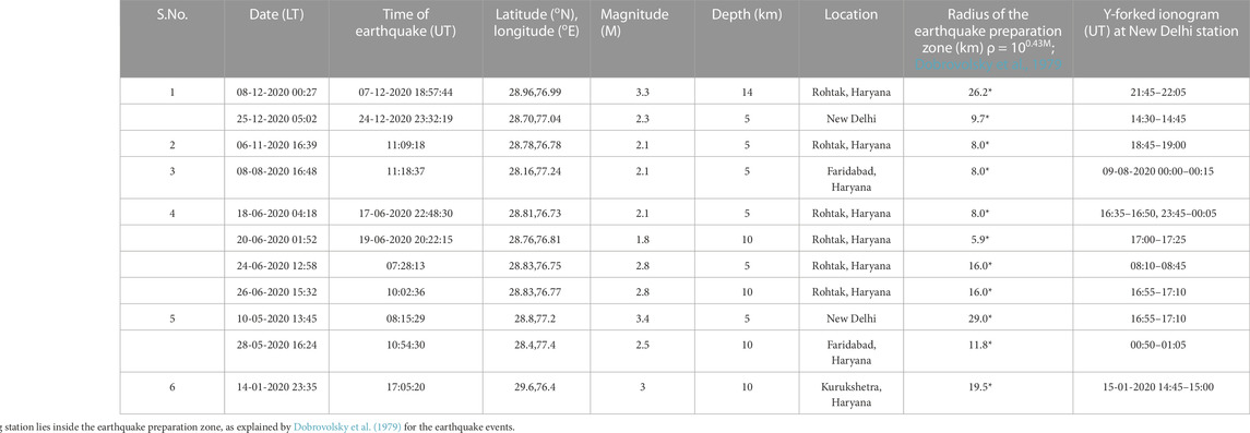
TABLE 1. Details of earthquake events affecting the low-mid latitude Indian station, New Delhi, during the year 2020 along with the ionogram records post-earthquake.

3.1 Earthquake event of 8 and 25 December 2020

3.1.1 Pre-earthquake analyses

On 8 December 2020, at 1857 UT, a magnitude 3.3 earthquake struck 38 km east of Rohtak, Haryana, India. The distance of the observing station at New Delhi (62 km) was well within the radius of the earthquake preparation zone (26 km) for this earthquake, and another earthquake of magnitude 2.3 struck with its epicenter in New Delhi itself on 25 December 2020, as shown in Table 1. The earthquake occurred on 8 December at 0027 LT (1857 UT of 7 December) and on 25 December 2020 at 0502 LT (2332 UT of 24 December). Figures 2A–D show the background space weather conditions and ionospheric F₂ region variations during this event. Figure 2A shows the interplanetary magnetic field’s Z component (Bz) ≥ −6.8 nT and solar wind speed (V_SW) under 634 km/s marked in blue, while Figure 2B shows the global geomagnetic storm index (Kp) < 4 and F10.7 cm flux in sfu (solar flux unit, 1 sfu = 10²² W/m²/Hz), well within 77–113 sfu, marked in blue from 24 November 2020 to 1 January 2021 (14 days before the first event and 7 days after the second earthquake event marked by the red line). The solar and geomagnetic disturbances shown in Figures 2A, B were quiet and steady before the earthquake, providing a perfect scenario for investigating any unusual ionospheric variations caused by this event.

FIGURE 2

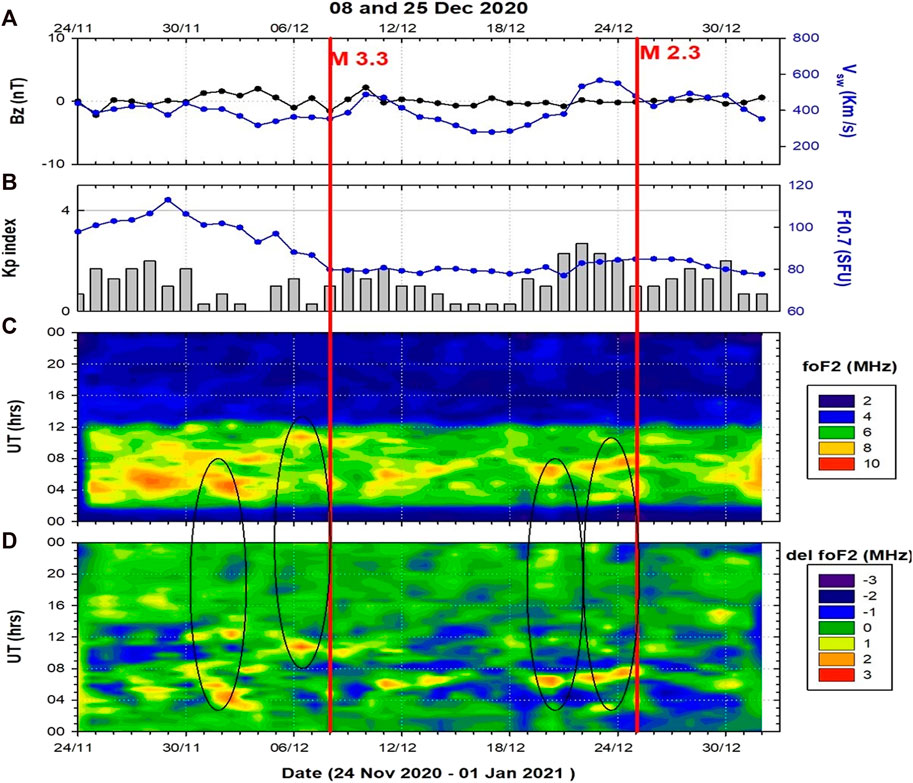
FIGURE 2. Plots of solar, geomagnetic, and ionospheric parameters from 24 November 2020 to 1 January 2021, 14 days before and 07 days after the earthquake events of 8 and 25 December 2020, showing (A) daily interplanetary magnetic field’s Z component (Bz) in nanotesla and solar wind speed (V_SW) in km/s in blue; (B) daily global geomagnetic storm index (Kp) and solar F10.7 flux in sfu (solar flux unit, 1 sfu = 10²² W/m²/Hz) given in blue; (C) variation in the F₂ layer critical frequency (f_oF₂) in MHz at low-mid latitude Indian station, New Delhi, observed every 5 min; and (D) deviation (Δf_oF₂) in MHz obtained by subtracting f_oF₂ values from the median of 10 quiet days.

To examine the ionospheric response of this earthquake event, the F₂ layer critical frequency (f_oF₂) for 39 days is shown in Figure 2C, covering the 14 days before and 7 days after the period of occurrence of both the earthquake events, i.e., from 24 November 2020 to 1 January 2021, as a function of time (UT). It can be noticed that enhanced f_oF₂ values are seen around 03–06 UT, followed by more pronounced f_oF₂ values (∼10 MHz) lasting for nearly 2 h at around 04–06 UT on 2 December 2020, the precursor day (marked by a circle), 6 days prior to the 8 December 2020 earthquake, and around 04–08 UT for the 25 December 2020 earthquake with pronounced f_oF₂ values around 9.2 MHz on 24 December 2020 (precursor day) and ∼9 MHz on 22 and 20 December 2020 (precursor days), i.e., 1, 3, and 5 days prior to the event (marked by a circle). This enhanced f_oF₂ variation, to be contemplated as anomalous, requires the day-to-day ionospheric variability to be removed from the observed f_oF₂ values. In view of this, Figure 2D presents the plot of the deviation of the F₂ layer critical frequency (Δf_oF₂) from quiet time ionospheric behavior during this period. It can be seen from this figure that a prominent enhancement, as large as ∼3 MHz, is noticed on 2 December 2020 between 04–06 UT and 12 UT, leading to ∼104% increase in the peak electron density at these times, and 2.5 MHz as noticed at 07–09 UT on 22 and 20 December 2020, leading to a 93% and 113% increase in electron density, respectively. The greatest enhancement and depression in electron density during this period were 127% and 63%, respectively. The maximum f_oF₂ variation during this period was ∼10 MHz, as shown in Figure 2C. It can also be seen that enhancements, not as prominent as they were on 2 December 2020, are also observed on 28 and 30 November and 4, 6, 11, 13, and 31 December 2020. It should be noted that there was a 4.2 magnitude earthquake on 17 December 2020 with its epicenter at Gurugram, Haryana, at 31.5 km from the observing station in New Delhi. Since the background space weather conditions as shown in Figures 2A, B were quiet during these periods of f_oF₂ variations, they could be due to this 4.2 magnitude impending earthquake. It is important to observe that prominent variations in f_oF₂ are observed a week prior to the earthquake event of 8 and 25 December 2020.

To better identify, visualize, and maintain an analogy with other reports, we present in Figure 3 a) hourly Dst variation, (b) Δf_oF₂ variation, (c) variation in F layer height (Δh'F) from quiet time median, and (d) percentage change in electron density from 24 November to 31 December 2020. It can be seen that the minimum Dst index was −13 nT at 10 UT on 8 December and −22 nT at 09 UT on 22 December 2020, indicating quiet geomagnetic conditions during this period. It can be clearly seen from the Δf_oF₂ plot in Figure 3B that the prominent enhancement of 3 MHz took place on 2 December 2020 (0400 UT) and 2.8 MHz on 20 December 2020 (0605 UT), as can be seen in Figure 2D. This enhanced ionospheric F₂ layer behavior indicates toward a precursory signal to the earthquake, which appeared at ionospheric height 6 days prior, resulting in a corresponding increase in electron density as high as ∼127%, as can be seen in Figure 3D. A meager variation of 2.6 MHz, as compared to 2 December 2020, was also observed on 6 December 2020, and a −2.17 MHz depression was observed on 21 December 2020, as depicted in Figure 3B.

FIGURE 3

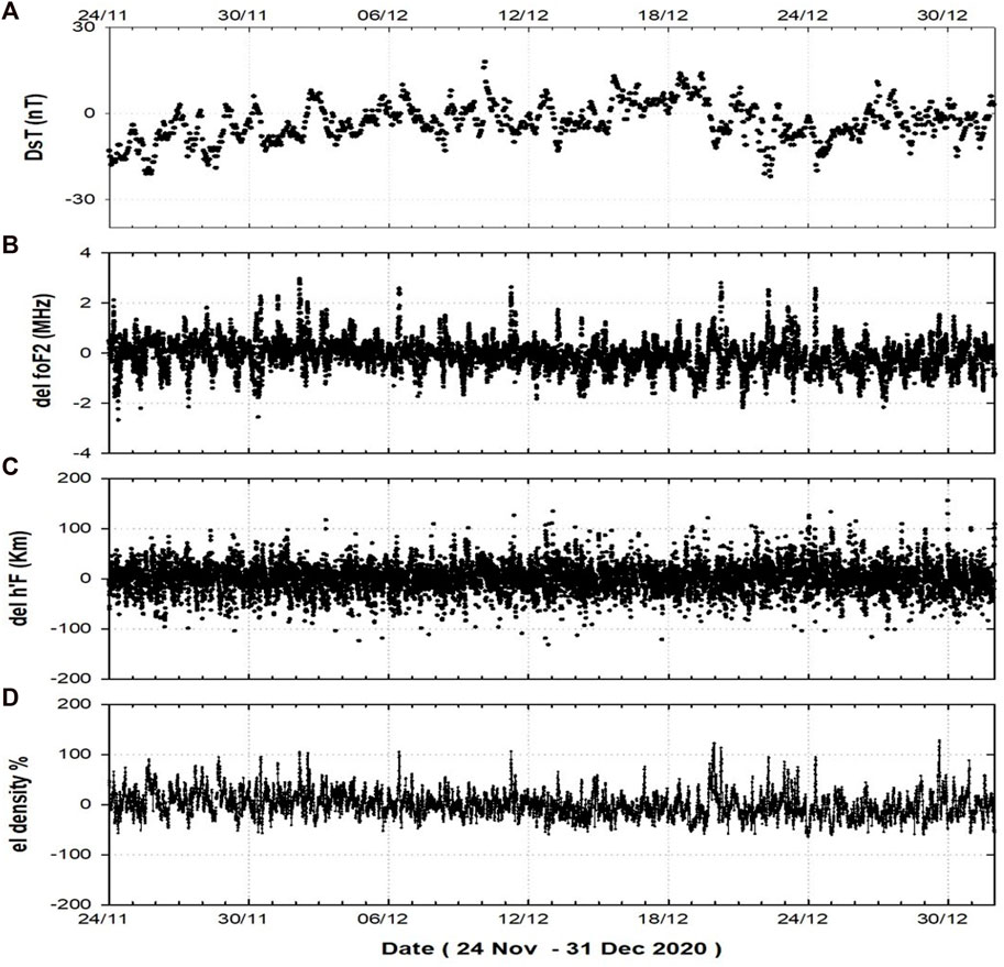
FIGURE 3. Plots of (A) hourly variation of the disturbance storm time index (Dst) in nanotesla; (B) deviation in the F₂ layer critical frequency (Δf_oF₂) from its quiet day median in megahertz; (C) deviation in the F layer peak height (Δh'F) from its quiet day median in kilometer, and (D) percentage variation in the electron density from 24 November to 31 December 2020.

Furthermore, instances of f_oF₂ variations were also observed after the earthquake events, enhancements (maximum of ∼43%) and depressions (maximum of ∼41%) on 9 December 2020 and depressions (maximum of ∼55%) on 27 December 2020. It is seen that at times when there was a maximum enhancement in Δf_oF₂ (on 2 December 2020), when the precursor is seen, no prominent variation (±50 km) in Δh'F was noticed, while ∼133 km variation in height is seen on 24 December 2020 (precursor day) for the 25 December 2020 earthquake, as is seen in Figure 3C. However, enhancements of the order of ∼117 km were observed in the evening time of 3 December 2020, and depressions of the order of ∼117 km were observed on a few occasions (e.g., in the evening time of 4, 5, and 7 December 2020), which were not followed by significant variations in Δf_oF₂. Furthermore, as data are available only for a week after the 25 December 2020 event, it is impossible to carry out further follow-up of the developments of the events.

3.1.2 Post-earthquake analysis

To check for post-earthquake ionospheric anomalies, we considered ionogram traces and distortions seen in the traces. Figure 4 shows the tracing of ionogram records post-earthquake event of 8 December 2020. The disturbances in the ionospheric plasma associated with the earthquake events mostly (but not always) manifest themselves in the data as a distinct Y-forking of the ionogram traces.

FIGURE 4

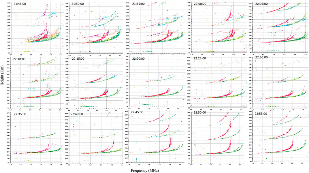
FIGURE 4. Sequential Y-forked ionograms (2145–2255 UT) at the NPL, New Delhi station, post the earthquake event of 8 December 2020 at 0027 UT. The ionogram traces in red color are those of O-mode polarization, and the traces in green color are those of X-mode polarization.

Figure 4 depicts a set of sample ionograms from the ionosonde station at New Delhi to highlight the appearance of the Y-forking signature post the earthquake event of 8 December 2020.

Y-forking of the ionogram was first observed at 21:45 UTC (Figure 4, first row), where the O-mode polarization can be seen to be split into two branches. Approximately 20 min later, Y-forking can be seen in both O- and X-mode ionogram traces, which lasts for up to 45 min, till the ionogram retrieves its original shape at 22:55UTC.

3.2 Earthquake event of 6 November 2020

This earthquake event of magnitude 2.1 on the Richter scale occurred in Rohtak, Haryana, on 6 November 2020 at 1109 UT. The distance of the ionospheric observing station in New Delhi, from the epicenter (∼62 km), was well within the radius of the earthquake preparation zone (∼1679 km), as can be seen from Table 1 along with its other details. The space weather conditions during this earthquake event are presented in Supplementary Figures S1A and S1B, from 23 October to 13 November 2020 (14 days before and 7 days after the earthquake). It can be seen from these plots that the solar and geomagnetic indices were quiet and stable, with B_Z ≥ −5.5 nT, solar wind velocity V_SW < 584 km/s, Kp below 4, and F10.7 cm flux varying from 71 to 92 sfu. Quite similar to the 8 December 2020 earthquake event, the space weather background conditions for the rest of the period are quiet, providing an ideal scenario to investigate changes imparted in F₂ layer critical frequency (f_oF₂), if any, due to this earthquake event. It can be seen from Supplementary Figure S1C that enhanced f_oF₂ values (∼12 MHz) were seen around 04–12 UT on 4 November 2020, nearly 2 days before the earthquake event. The enhancements can be better visualized in Supplementary Figure S1D, where we present a plot of deviation in the F₂ layer critical frequency from the quiet time behavior (Δf_oF₂). It shows a prominent enhancement (∼3 MHz) around 1330 UT on 4 November 2020, followed by a more pronounced enhancement (∼5 MHz) located around ∼1030 UT on 4 November 2020 (marked by a circle). The electron density increased by ∼229% on 4 November 2020, 2 days prior to the earthquake, at the ionospheric monitoring station in New Delhi. Other enhancements in f_oF₂ of lesser intensity were also observed on 24, 26, 28, and 29 October and 1 November 2020. Apart from this, instances of depressions as observed for the 8 December 2020 earthquake event can also be seen on earthquake days at 04 UT and 26 October–1 November 2020 around 12–15 UT, as well as at 5 UT on 1 November 2020. The maximum depression (∼4 MHz) corresponds to ∼81% decrease in electron density, as can be seen in Supplementary Figure S2D. Similar to Figure 4, Supplementary Figure S2A shows the Dst variation during 31 October–6 November 2020 (a week prior to the earthquake). A minimum value of −35 nT on 31 October 2020 was observed during this period, indicating quiet geomagnetic conditions.

The day-to-day variation plot of Δf_oF₂ during 31 October–6 November 2020 in Supplementary Figure S2B depicts the enhanced variations of 2 and 5.2 MHz on 3 November 2020 (around 1035 UT) and on 4 November 2020 (around 09 UT), respectively, as also shown in Supplementary Figure S1D. It can be seen from Supplementary Figure S2C that the deviation from quiet time behavior of the F₂ layer peak height (Δh'F) from 31 October to 6 November 2020 varies within ±100 km. However, the maximum increase in Δf_oF₂ on 4 November 2020 (Supplementary Figure S2B) does not cause much change in Δh'F. More instances of enhancements in h'F are seen before the event and vice versa after the event; however, the magnitude of variations is less than that of f_oF₂ variations.

3.2.1 Post-earthquake analysis

The Y-forking signature for this earthquake event of 6 November 2020 (1109 UT) was first observed at 1845 UT, i.e., approximately 6 h and 45 min after the earthquake. A prominent splitting of O-mode polarization and a slight hint of splitting in X-mode polarization can be seen in Supplementary Figure S3. The anomaly lasted for 15 min, after which the ionogram regained its original shape.

3.3 Earthquake event of 8 August 2020

The epicenter of this earthquake event of magnitude 2.1 was in Faridabad, Haryana, at 1118 UT, at a distance of ∼57 km from theionospheric monitoring station in New Delhi. The space weather indices are shown in Supplementary Figures S4A and S4B, from 25 July to 15 August 2020 (14 days before and 7 days after the earthquake on 8 August 2020). B_Z showed no variation, the solar wind velocity was at its lowest with a maximum value reaching ∼643 km/s on 4 August 2020, 4 days before the earthquake. The Kp index was <4, the F10.7 cm solar flux ranged from 72 to 76 sfu, and the Dst index had normal values. It can be seen from Supplementary Figure S4C that f_oF₂ shows an increase from 06 to 15 UT during this period of analysis. Enhanced f_oF₂ values were primarily seen on 6 August 2020 around 1030 UT (marked by a circle) and on 4 August 2020 around 0830 UT. It can be seen from Supplementary Figure S4D, in which the variation of f_oF₂ (Δf_oF₂) from the normal quiet time is shown, that a prominent enhancement of ∼3.3 MHz occurred on 6 August 2020, primarily confined to 07–10 UT. Instances of depressions in between enhancements, as seen during the 6 November 2020 and 8 December 2020 earthquakes, are quite evident during this earthquake event, on 30 July and 1, 3, and 5 August 2020 (within a week before the earthquake) and on 9 and 14 August 2020 (within a week after the earthquake event). A maximum variation of ∼160% in electron density is observed during this earthquake event. Other lesser intensity enhancements are observed on 25, 27, and 31 July and 2, 8, 10, and 12 August 2020, as also seen in Supplementary Figure S4C. The increased geomagnetic conditions around 2 and 3 August 2020, as shown in Supplementary Figures S4A and S4B could have resulted in the anomalous variation in f_oF₂ around 2 August 2020. It is important to note that another 3 and 2.9 magnitude earthquakes occurred on 24 July and 5 August 2020, respectively, with their epicenters closer to the observing station, New Delhi. The anomalous ionospheric perturbations could be attributed to these earthquakes. To precisely locate the time of enhancement, in Supplementary Figure S5, we have shown Δf_oF₂ variation in Supplementary Figure S5B during 2–8 August 2020, along with the Dst index variation in Supplementary Figure S5A during the corresponding times. It can be seen that a prominent enhancement (3.3 MHz) is seen around 0815 UT on 6 August 2020 and around 1205 UT on 4 August 2020. It is important to point out here that an enhancement of nearly 3 MHz is seen quite a few times during this period, whereas the maximum depression of 3.2 MHz is observed at 1440 UT on 3 August 2020. To examine the response of F₂ layer peak height (h'F), Supplementary Figure S5C shows Δh'F variation during this period, which varies within ±100 km. However, it shows an opposite response to variation in Δf_oF₂, as the maximum enhancement in Δf_oF₂ on 6 August 2020 shown in Supplementary Figure S5B (precursor to the earthquake) corresponds to a depression in Δh'F variation with a maximum decrement to ∼124 km on 6 August 2020.

3.3.1 Post-earthquake analysis

The Y-forking signature for this earthquake event of 8 August 2020 (1118 UT) was first observed at 0000 UT of 9 August 2020, i.e., approximately 12 h and 40 min after the earthquake. A prominent splitting of O-mode and X-mode polarizations can be seen in Supplementary Figure S6. The anomaly lasted for 15 min, after which the ionogram regained its original shape.

3.4 Earthquake events of 18, 20, 24, and 26 June 2020

Four earthquakes occurred 62 km from New Delhi in June: on 18 (04:18 LT or 22:48 UT of 17 June 2020), 20 (0152 LT or 20:22 UT of 19 June 2020), 24 (1258 LT or 0728 UT), and 26 (1532 LT or 1002 UT) June 2020 with epicenters in Rohtak, Haryana, measuring 2.1, 1.8, 2.8, and 2.8, respectively. To investigate the ionospheric response during these occurrences, the background space weather conditions are depicted in Supplementary Figures S7A and S7B using the indices B_Z, V_SW, and Kp and F10.7 cm, during the period of 4 June to 3 July 2020 (14 days before and 7 days after the earthquake events). The plots show normal Bz values during this period, with a maximum of 5.9 nT on 27 June 2020 at 1100 UT, solar wind velocities V_SW of 540 km/s, Kp below 4, and solar flux ranging from 69 to 75 sfu. These space weather variant results imply that the background conditions were stable.

The F₂ layer critical frequency variations during 4 June to 3 July 2020 are shown in Supplementary Figure S7C. The enhanced f_oF₂ values (∼9.5 MHz) are seen around 04–16 UT. These enhancements can be clearly observed in Supplementary Figure S7D, where deviations in f_oF₂ (Δf_oF₂) from the normal quiet days during this period are shown. Perceptible f_oF₂ variations are seen on 16, 20, and 24 June 2020. A prominent enhancement of ∼2.75 MHz is observed on 16 June 2020 and ∼4 MHz on 24 June 2020, while depressions are seen on 13, 16, 18, 20, 23, and 24 June 2020 during this period. The electron density increased by ∼196% during this period, as can be seen in Supplementary Figure S8D. The large variations observed after the earthquake period, starting from 27 June 2020, are because of the earthquake events of 27 and 30 June 2020, as the Dst index in Supplementary Figure S8A remained above 30 nT, indicating quiet background conditions. These enhanced variations can be precisely seen in Supplementary Figure S8B, where Δf_oF₂ values are shown during 12 June–26 June 2020 (a week before the events). The enhancements, as also seen in Supplementary Figure S7D, are observed here on 16 June 2020 (2.75 MHz at 1235 UT) seen 2 days prior to the 18 June 2020 earthquake event; 18 June 2020 (2.1 MHz at 1155 UT) seen 2 days prior to the 20 June 2020 earthquake event; 20 June 2020 (2.4 MHz at 1405 UT) seen 4 days prior to the 24 June 2020 earthquake event; and 24 June 2020 (3.9 MHz 1205 UT) seen 2 days prior to the 26 June earthquake event. It is important to note that a depression of 2.2 MHz was also seen on 24 June 2020, which was the earthquake day, at 0640 UT, depressions of 1.8 MHz at 1600 UT and 1.9 MHz at 0645 UT were also seen on 20 and 26 June 2020, respectively, which were other earthquake days. Supplementary Figure S8C shows the F₂ layer height deviation (Δh'F) from quiet time behavior, varying within ±200 km. Corresponding to the increase in Δf_oF₂ on 16 June 2020 as sown in Supplementary Figure S8B (precursor day), there is no prominent variation (±50) noticed in Δh'F. This is contrary to the earthquake case of 28 May 2020, where there was a negative response in hmF₂ corresponding to the respective precursor day’s maximum enhancement in Δf_oF₂.

3.4.1 Post-earthquake analysis

The Y-forking signature for this earthquake event of 18 June 2020 (04:18 LT or 22:48 UT of 17 June 2020) was first observed at 1635 UT, i.e., approximately 17 h and 45 min after the earthquake. A prominent splitting of O-mode and X-mode polarizations can be seen in Supplementary Figure S9A. The anomaly lasted for 15 min, after which the ionogram regained its original shape.

The Y-forking signature for this earthquake event of 20 June 2020 (0152 LT or 20:22 UT of 19 June 2020) was first observed at 1700 UT, i.e., approximately 21 h after the earthquake. A prominent splitting of O-mode and X-mode polarization can be seen in Supplementary Figure S9B. The anomaly lasted for 15 min, after which the ionogram regained its original shape.

The Y-forking signature for this earthquake event of 24 June 2020 (0728 UT) was first observed at 08:15 UT, i.e., approximately 40 min after the earthquake. A prominent splitting of O-mode and X-mode polarization can be seen in Supplementary Figure S9C. The anomaly lasted for 15 min, after which the ionogram regained its original shape.

The Y-forking signature for this earthquake event of 26 June 2020 (1002 UT) was first observed at 1655UT, i.e., approximately 7 h after the earthquake. A prominent splitting of O-mode and X-mode polarization can be seen in Supplementary Figure S9D. The anomaly lasted for 15 min after which the ionogram regained its original shape.

3.5 Earthquake events of 10 and 28 May 2020

Several earthquakes of magnitude <4 struck New Delhi and the surrounding areas in May. On 10 May 2020 at 0815 UT, a 3.4 magnitude earthquake struck and on 28 May 2020 at 1054 UT, a 2.5 magnitude earthquake struck, with the epicenter in Faridabad, Haryana, about 28 km from the monitoring station in New Delhi. The background conditions are depicted in Supplementary Figures S10A and S10B from 26 April 2020 to 4 June 2020, to look for space weather events that could disrupt the ionosphere (14 days before and 7 days after the earthquake event). The maximum Kp was 3.3, the solar flux F10.7 cm was 72.8, and the solar wind velocity, V_SW, was less than 500 km/s, indicating quiet background solar and geomagnetic conditions.

Supplementary Figure S10C shows the variation in f_oF₂ from 26 April 2020 to 4 June 2020. There was a prominent increase on 27 April 2020, when f_oF₂ reached ∼10 MHz, and on 1 May 20, when f_oF₂ reached ∼10.45 MHz around 08–13 UT. It is important to note that due to the non-availability of data from 2 to 8 May 2020, the variation just a week before the 10 May 2020 earthquake event could not be studied. Deviations in f_oF₂ (Δf_oF₂) from normal quiet medians, shown in Supplementary Figure S10D, present enhancements, as also seen in Supplementary Figure S10C on 27 April and 1 and 9 May 2020. Supplementary Figure S11B clearly shows the variation in Δf_oF₂ values from 26 April 2020 to 4 June 2020 (a week before the earthquake), along with the geomagnetic conditions (Supplementary Figure S11A). In line with Supplementary Figure S10D, Supplementary Figure S11B shows enhanced Δf_oF₂ values on 27 April 2020 (2.6 MHz at 1255 UT) and 1 May 2020 (4.9 MHz at 1240 UT), along with the maximum depression of 3.8 MHz on 28 April 2020 at 0705 UT. A maximum increase of ∼266% and a maximum decrease of ∼75% in electron density are observed during this event, as shown in Supplementary Figure S11D. Supplementary Figure S11C shows the deviation of the F₂ layer height from normal quiet time behavior (Δh'F). It can be seen that Δh'F varies within ±200 km from 26 April 2020 to 4 June 2020. It is important to point out that no prominent variation in F layer height is observed corresponding to the enhanced critical frequency on the precursor day (1 May 2020). This is similar to the earthquake cases of June 2020, as explained in the previous section.

Similarly, for the earthquake event of 28 May 2020 at 1054 UT, a prominent increase in f_oF₂ of 8.8 MHz at 1240 UT was seen on 25 May 2020 (precursor day) with a corresponding Δf_oF₂ of 3.3 MHz, as can be seen in Supplementary Figure S10D. A pronounced increase in electron density of 160% is evidenced for this precursor day.

A maximum decrease of 3.14 MHz in f_oF₂ variation and a maximum decrease of 75% in electron density are observed during this period. A fall of ∼100 km in F layer height is observed during this period. It is important to note that several earthquakes of magnitude 4.5 and less occurred on 3, 29, and 31 May 2020 to which the enhancements and depression on 12, 14, 21, and 31 May 2020 can be attributed, as the other solar and geomagnetic conditions remained stable during this period.

The Y-forking signature for the earthquake events of 10 and 28 May 2020 both lasted for 15 min with significant Y-forking signatures, as shown in Supplementary Figures S12A and S12B.

3.6 Earthquake event of 14 January 2020

An earthquake measuring magnitude 3 on the Richter scale hit 61 km SW of Kurukshetra, Haryana, India, on 14 January 2020 around 1705 UT. To look for space weather events, as they can also perturb the ionosphere, the background conditions are shown in Supplementary Figures S13A and S13B, from 31 December 2019 to 21 January 2020 (14 days before and 7 days after the earthquake event). The interplanetary magnetic field (Bz), Kp, solar wind velocity (V_SW), and F10.7 cm solar flux remained stable and low throughout the period; thus, the ionospheric response to the earthquake event of 14 January 2020 can be expected to be unambiguous.

Supplementary Figure S13C shows the variation in F₂ layer critical frequency (f_oF₂) from 31 December 2019 to 21 January 2020. There was a prominent increase on 9 and 11 January 2020, where f_oF₂ reached ∼8 MHz, around 03–12 UT. Other enhanced f_oF₂ values can be observed on 3, 6, and 13 January 2020 around 03–12 UT. Deviations in f_oF₂ (Δf_oF₂) from normal quiet medians, presented in Supplementary Figure S13D, show enhancements as also shown in Supplementary Figure S13C on 3, 6, 9, 11, and 13 January 2020. Supplementary Figure S14B clearly shows the variation in Δf_oF₂ values from 8 January 2020 to 14 January 2020 (a week before the earthquake), along with the geomagnetic conditions. In line with Supplementary Figure S13D, Supplementary Figure S14B shows enhanced Δf_oF₂ values on 9 January 2020 (∼3 MHz at 0540 UT) and 11 January 2020 (2.9 MHz at 0355 UT), along with the maximum depression of 1.3 MHz on 12 and 14 January 2020 at 09–11 UT. A maximum increase of ∼166% in electron density is observed during this event (Supplementary Figure S14D). Supplementary Figure S14C shows the deviation of F₂ layer peak height from normal quiet time behavior (Δh'F). It is important to point out that ∼125 km variation in the peak height is observed, corresponding to the enhanced critical frequency on the precursor day (9 January 2020).

3.6.1 Post-earthquake analysis

The Y-forking signature for this earthquake event of 14 January 2020 (1705 UT) was first observed at 1445 UT of 15 January 2020, i.e., approximately 21 h and 40 min after the earthquake. In Supplementary Figure S15, a prominent Y-forking signature in O-mode polarization can be seen. The anomaly lasted for 15 min, after which a normal ionogram trace reappeared.

4 Discussion

At low or low-mid latitudes, the ionosphere, apart from being influenced by the equatorial electric field, is affected by geomagnetic disturbances originating from solar–terrestrial interactions. The equatorial plasma drift is a manifestation of direct penetrating electric fields and long-lasting disturbed dynamo electric fields. The sharp changes in the interplanetary magnetic field can result in prompt penetration of electric fields; hence, solar wind and magnetospheric driving mechanisms influence the equatorial and low-latitude ionosphere significantly during geomagnetic storms. During our examination of the ionospheric responses, we noticed that the interplanetary magnetic field (Bz), geomagnetic indices (Kp and Dst), and variations in solar wind speed (Vsw) remained relatively quiet and stable. As a result, the noticeable disturbances observed are believed to be disassociated from geomagnetic conditions or equatorial dynamics.

The investigation of the ionospheric response of the F₂ region to the 11 earthquake events during the year 2020 with magnitudes of less than 4 as recorded on the Richter scale at a low-mid latitude Indian station, New Delhi, has shown that there are perceptible ionospheric variations ranging from 2 to 9 days prior to these earthquakes. A detailed summary of observations, depicting the maximum and minimum F₂ layer critical frequencies (f_oF₂), its maximum and minimum deviations (Δf_oF₂) from quiet time behavior, the maximum and minimum changes in electron density, and the number of days prior to the event when maximum variations were noticed is presented in Table 2. It can be seen from the table that a maximum enhancement varying from ∼122% to 266% and a maximum depression ranging from ∼55% to 76% in electron density occurred during these events. Furthermore, we found significant occurrences of enhancements in comparison to depressions in the F₂ region critical frequency at a low-mid latitude Indian station, New Delhi. A few of the selected electron density profiles on the precursor day are plotted in Figure 5 along with five quiet day profiles at approximately similar timings for the four earthquake events. It can be seen from the figure that the maximum peak electron density varies by a factor of 1.6–1.9 on the precursor day (shown in black) for these four earthquake events. However, the altitude does not change much on the precursor day from the quiet time average variation. There are changes in altitude on the earthquake day (event day); however, these changes are not as prominent as are seen in the frequencies (more than 250%), which are reported by us and in most of the reports as mentioned in the article. The main ionospheric variations that are being observed occur prior to earthquakes, and the behavior of ionospheric altitude (h'F) in relation to seismic events is a complex phenomenon that is not fully understood. It is established that some earthquakes can trigger disturbances in the ionosphere, causing changes in h'F. However, not every earthquake will necessarily have such effects. Several factors play a role, such as the magnitude and depth of the earthquake (smaller or deeper earthquakes may have a minimal or undetectable impact on the ionosphere), the radius of the earthquake preparation zone (effects may be unnoticed if the earthquake lies outside the radius of the earthquake preparation zone), and the specific ionospheric conditions at the time (pre-existing disturbances or irregularities may overshadow earthquake-induced effects). It is important to emphasize that the study of ionospheric responses to earthquakes is an ongoing research field, and researchers are continuously exploring the connection between seismic events and ionospheric disturbances. While progress has been made in understanding this relationship (a causative mechanism), it remains a complex and multifaceted area influenced by various factors.

TABLE 2

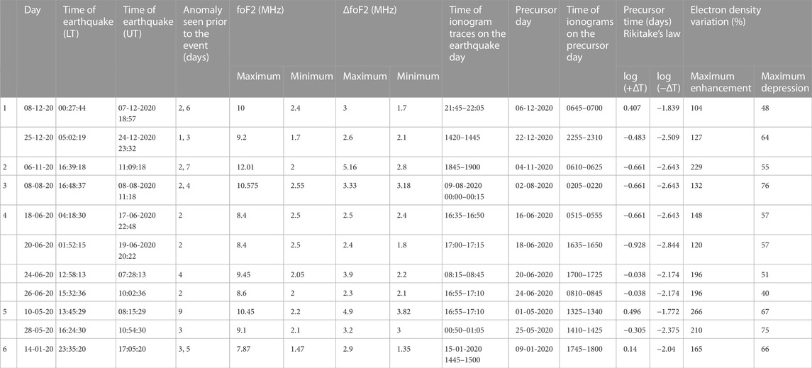
TABLE 2. Details of earthquake events along with their precursor day and Y-forked ionogram.

FIGURE 5

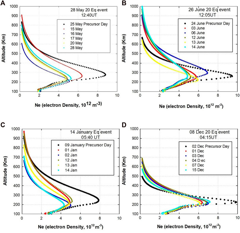
FIGURE 5. Plot showing electron density profiles of precursor day and 5 quiet days of the month for the earthquake events of (A) 28 May 2020, (B) 26 June 2020, (C) 14 January 2020, and (D) 08 December 2020.

Few reports of ionospheric perturbations have been observed from the ionospheric monitoring station in New Delhi prior to earthquakes. In an earlier study (Gupta and Upadhayaya, 2017), perceptible ionospheric variations leading to peak electron density variations of ∼207% were reported while investigating the ionospheric response to five major earthquake events that were greater than 6 on the Richter scale, affecting a low-mid latitude Indian station, New Delhi, during the years 2015 and 2016. In another study, Sharma et al. (2010) reported anomalous enhancement in the ionospheric TEC and f_oF₂ 1–4 days before the main shock during three major earthquakes (M > 6) in China in the year 2008. Dabas et al. (2007) also reported unusual ionospheric variations (both enhancements and depressions) in f_oF₂ values varying from 1 to 25 days prior to the occurrence of 11 major earthquakes (M > 6) that occurred in the Asian region. These studies reported perceptible ionospheric perturbations and indicated the possibility of seismo-ionospheric coupling. In this study, we have found that even lower magnitude earthquakes (M < 4) seem to affect electron densities in the ionosphere before an impending earthquake when the ionospheric monitoring station is near the epicenter. It is important to emphasize that while there is evidence of ionospheric anomalies preceding earthquakes, the exact mechanisms and causal relationships are still not fully understood. One possible explanation could be the generation of a powerful electric field in the vicinity of the Earth’s surface. Pulinets et al. (1994) proposed a coupling model providing a block diagram of the seismo-ionospheric coupling mechanism that suggested that radon is emitted from the region where the earthquake’s epicenter is located, both during and preceding the occurrence of the earthquake. Another similar schematic depiction of the causative mechanism has been reported by Revathi et al. (2010), Kuo et al. (2015), and Xiong et al. (2021b). The increased concentration of ions in the seismic zone initiates a process known as nucleation, leading to the formation of ion clusters (Pulinets and Ouzounov, 2011). The diffusion of radon is facilitated by carbon dioxide and methane (Khilyuk et al., 2000), which in turn incite the generation of acoustic gravity waves. The movement of air disrupts the ion clusters, causing a rapid enrichment of ions in the near-Earth atmosphere. Consequently, an anomalously strong vertical electric field of approximately 1 kV/m magnitude is produced through a process of charge separation. This intense electric field can penetrate the ionosphere, altering its dynamics and electron density (Pulinets et al., 2000). The physical mechanisms of pre-seismic anomaly generation are suggested in the framework of the LAIC model (Freund, 2011; Pulinets and Ouzounov, 2011; De Santis et al., 2015; 2019). However, further research and monitoring are required to establish the validity and reliability of ionosphere–earthquake coupling as a predictive tool for earthquakeforecasting.

The three vital parameters of an earthquake are its magnitude, depth, and distance from the epicenter. The ionospheric variations prior to an earthquake are reported chiefly and believed to be observed for stronger earthquakes (M > 6) and weaker earthquakes (M < 4.2) that are not likely to perturb the ionosphere (Liu et al., 2006). It is also believed that earthquakes with hypo-central depths within 50 km are likely to affect the ionosphere (Molchanov and Hayakawa, 1998). However, by contrast, we have observed ionospheric perturbations prior to earthquakes of M < 4. In our analysis, we found three cases: 18 June 2020, 8 August 2020, and 8 December 2020, where the magnitude and depth were the same. However, it is important to note that electron density variations of 120%, 132%, and 229% were observed. These observations point toward the complexity and thus the elusiveness of the F region ionosphere (Rishbeth, 2000; Mendillo et al., 2001). Furthermore, it is proposed that the precursor time (ΔT) in days is related to the magnitude of the earthquake by the empirical law log₁₀(ΔT) = a + bM (Rikitake, 1987), where M is the magnitude of the earthquake event and a and b are constants. In view of the above, we examined the earthquake events and calculated the precursor time by taking values of a = −3.29 (±0.76) and b = 0.78 (±0.11), as incorporated by De Santis et al. (2019) in their study on the analysis of electron density from the swarm satellites. As seen from Table 2, the time of the precursor is found to be 1–3 days for these earthquake events; however, in our observations of F₂ layer critical frequency, the precursors are mostly seen varying from 2 to 9 days during these events. Furthermore, as can be seen from Figure 6, a linear relationship between the precursor time and magnitude of an earthquake is seen for weaker earthquakes measuring less than 4 that are within the radius of the earthquake preparation zone. This result suggests that the precursor times are related to the magnitude of the earthquakes; however, a comprehensive study of the dependency of parameters like depth, magnitude, and distance from the epicenter on the precursor time is thus suggested as a potentially productive line of inquiry.

FIGURE 6

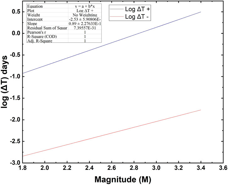
FIGURE 6. Plot showing relationship between earthquake magnitude and precursor time using Rikitake’s law.

TIDs of various scale sizes are produced in the thermosphere because of gravity waves, which play a vital role in the transportation of energy from above and below. TIDs appear as signatures in distorted ionograms that have unusual splitting or Y-forking. In our analysis of earthquake events, we have predominantly observed the Y-forking of the ionograms in both the O and X modes of polarization near the F₂ layer frequency on the event and precursor days, as seen in Figure 7. It is important to note that in some cases, we have also observed opposite Doppler shifts in both the O and X modes. Furthermore, we have found large vertical displacements along with sharp descents following sharp rises when Y-forking in ionograms was observed in comparison to that on other days. Figure 8 shows the case of 8 December 2020, where a large variation (∼90 km) in the virtual height is seen when Y forking is observed in comparison to the previous day where a variation of ∼50 km is seen. As propagation of TIDs may cause undulations in the F layer height as a consequence of spread in the height and/or frequency in the ionograms ( Shiokawa et al., 2003; Lakshmi Narayanan et al., 2014; Yadav et al., 2021a; 2021b; Rathi et al., 2021; 2022). These sharp variations observed in the virtual height point toward the passage of TIDs over the ionospheric monitoring station in New Delhi. In order to ascertain the presence of TIDs, we have used O(¹D) 630.0 nm airglow data from a multi-wavelength all-sky airglow imager installed at Hanle, Ladakh, India (32.7°N, 78.9°E; dip lat. ∼24.1°N), as the Digisonde lies at the southern edge of the airglow imager’s field of view (FOV), having a partially common volume region of observation in the ionosphere. Figure 9 represents the unwarped O(¹D) 630.0 nm all-sky airglow images during moonless and clear sky conditions for the events when the data were available. We can observe a faint plasma structure likely to be MSTID on the event nights (18 and 20 June 2020) and the precursor nights (10 and 16 June 2020), which sustained for more than 40 min during each night. These structures appeared in the northeast of the imager’s FOV and propagated southeastward. We have estimated the horizontal velocities of the whole plasma structure for all the nights, which are 62.03 ± 7.17 m/s, 90.3 ± 11.4 m/s, 95.53 ± 7.13 m/s, and 60.93 ± 2.6 m/s for 18 June 2020, 20 June 2020, 10 June 2020, and 16 June 2020, respectively. The horizontal velocities of these MSTIDs are similar to those of other events from the same locations reported previously (Yadav et al., 2021a; Yadav et al., 2021b; Rathi et al., 2021; Rathi et al., 2022). Similar Y-forking in ionograms was earlier reported from I-Cheon, Korea, a few hours after the 11 March 2011 Tohoku earthquake and by the meteor explosion event over Chelyabinsk on 15 February 2013 (Pradipta et al., 2015). In their study, the authors reported the presence of Y-forked ionograms as a signature of TIDs, which is supposed to have been caused by the meteor explosion. This is important to point out that Y-forked ionograms during the period (7 and 8 December 2020) of the study were also seen at Trivandrum and Ahmedabad, as shown in Figure 10.

FIGURE 7

FIGURE 7. Plot showing Y-forked signature in ionogram traces on the precursor day.

FIGURE 8

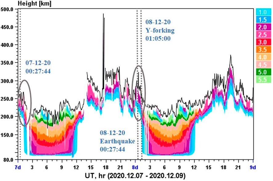
FIGURE 8. Plot showing earthquake event of 8 December 2020, where a large variation (∼90 km) in the virtual height is seen when Y-forking is observed in comparison to that of the previous day, where a variation of ∼50 km was seen.

FIGURE 9

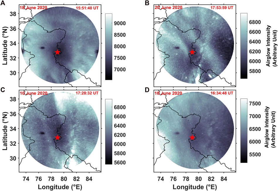
FIGURE 9. Plot of the unwarped O(¹D) 630.0 nm all-sky airglow images during moonless and clear sky conditions for the earthquake event nights of (A) 18 June 2020 and (B) 20 June 2020 and the precursor nights of (C) 10 June 2020 and (D) 16 June 2020.

FIGURE 10

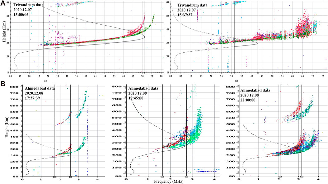
FIGURE 10. Plot of Y-forked ionograms at (A) Trivandrum and (B) Ahmedabad on 7 and 8 December 2020.

5 Conclusion

Based on our investigation on the extent of ionospheric changes following 11 earthquake events measuring less than 4 on the Richter scale during the year 2020 in the vicinity of New Delhi (28.6°N, 77.2°E, 42.4°N dip), the following conclusions are drawn:

1) There are perceptible ionospheric perturbations 2 to 9 days before the event that can be linked to these earthquakes.

2) These perturbations resulted in a peak electron density of more than 250% when compared to the quiet time ionosphere for earthquakes measuring less than 4 on the Richter scale when the ionospheric monitoring station was in the vicinity of the epicenter.

3) A linear relationship between the precursor time and magnitude, as suggested by Rikitake’s (1987) empirical law, was observed.

4) Y-forked ionograms with opposite Doppler shifts in both O- and X-mode polarizations were observed before and after the earthquake events at New Delhi. Traces of Y-forked ionograms were also seen in Ahmedabad andTrivandrum.

5) These Y-forked ionograms are one of the characteristic signatures of TIDs moving with a horizontal velocity varying from 60 to 100 m/s.

Data availability statement

The raw data supporting the conclusion of this article will be made available by the authors, without undue reservation.

Author contributions

AB, AG, QA, AS, and SG analyzed the New Delhi digisonde data and prepared the figures. SS, MS, DP, and TP analyzed the Roorkee, Trivandrum, and Ahmedabad data and discussed the results. AU and AB wrote the manuscript. All authors contributed to the article and approved the submitted version.

Acknowledgments

The authors thank the World Data Center, Kyoto University, Kyoto, Japan, for geomagnetic indices data Dst (omniweb.gsfc.nasa.gov/form/dx1.html). The Z component of the interplanetary magnetic field Bz in the geocentric solar magnetospheric (GSM) coordinate has been downloaded from the National Space Science Data Center, NASA/Goddard website. AB, AU, and QA are thankful to UGC, and AS is thankful to CSIR for granting the Senior Research Fellowship. The authors thank CSIR for providing the facilities. They also thank CSIR-NPL for providing facility to work. SS acknowledges the financial support from the Science and Engineering Research Board, Department of Science and Technology, Government of India (CRG/2021/002052), to maintain the multi-wavelength airglow imager. The support from Indian Astronomical Observatory (operated by the Indian Institute of Astrophysics, Bengaluru, India), Hanle, Ladakh, India, for the day-to-day operations of the imager is duly acknowledged. One of the author, SS, is thankful to Dipjyoti Patgiri for producing the unwarped images for four nights and estimating the velocities. This work is also supported by the Ministry of Education and Department of Space, Government of India.

Conflict of interest

The authors declare that the research was conducted in the absence of any commercial or financial relationships that could be construed as a potential conflict of interest.

Publisher’s note

All claims expressed in this article are solely those of the authors and do not necessarily represent those of their affiliated organizations, or those of the publisher, editors, and reviewers. Any product that may be evaluated in this article, or claim that may be made by its manufacturer, is not guaranteed or endorsed by the publisher.

Supplementary material

The Supplementary Material for this article can be found online at: https://www.frontiersin.org/articles/10.3389/fspas.2023.1170288/full#supplementary-material

References

Artru, J., Farges, T., and Lognonné, P. (2004). Acoustic waves generated from seismic surface waves: Propagation properties determined from Doppler sounding observations and normal-mode modelling: Propagation of seismic acoustic waves. Geophys. J. Int. 158, 1067–1077. doi:10.1111/j.1365-246X.2004.02377.x

CrossRef Full Text | Google Scholar

Astafyeva, E., Heki, K., Kiryushkin, V., Afraimovich, E., and Shalimov, S. (2009). Two-mode long-distance propagation of coseismic ionosphere disturbances. J. Geophys. Res. Space Phys. 114. doi:10.1029/2008JA013853

CrossRef Full Text | Google Scholar

Blanc, E. (1985). Observations in the upper atmosphere of infrasonic waves from natural or artificial sources - a summary. Ann. Geophys. 3, 673–687. Available at: https://ui.adsabs.harvard.edu/abs/1985AnGeo.3.673B (Accessed January 6, 2023).

Google Scholar

Bolt, B. A. (1964). Seismic air waves from the great 1964 alaskan earthquake. Nature 202, 1095–1096. doi:10.1038/2021095a0

CrossRef Full Text | Google Scholar

Chum, J., Hruska, F., Zednik, J., and Lastovicka, J. (2012). Ionospheric disturbances (infrasound waves) over the Czech Republic excited by the 2011 Tohoku earthquake. J. Geophys. Res. Space Phys. 117. doi:10.1029/2012JA017767

CrossRef Full Text | Google Scholar

Dabas, R. S., Das, R. M., Sharma, K., and Pillai, K. G. M. (2007). Ionospheric pre-cursors observed over low latitudes during some of the recent major earthquakes. J. Atmos. Solar-Terrestrial Phys. 69, 1813–1824. doi:10.1016/j.jastp.2007.09.005

CrossRef Full Text | Google Scholar

De Santis, A., De Franceschi, G., Spogli, L., Perrone, L., Alfonsi, L., Qamili, E., et al. (2015). Geospace perturbations induced by the Earth: The state of the art and future trends. Phys. Chem. Earth 85-86, 17–33. Parts A/B/C 85–86. doi:10.1016/j.pce.2015.05.004

CrossRef Full Text | Google Scholar

De Santis, A., Marchetti, D., Pavón-Carrasco, F. J., Cianchini, G., Perrone, L., Abbattista, C., et al. (2019). Precursory worldwide signatures of earthquake occurrences on Swarm satellite data. Sci. Rep. 9, 20287. doi:10.1038/s41598-019-56599-1

PubMed Abstract | CrossRef Full Text | Google Scholar

Dobrovolsky, I. P., Zubkov, S. I., and Miachkin, V. I. (1979). Estimation of the size of earthquake preparation zones. PAGEOPH 117, 1025–1044. doi:10.1007/BF0087-6083

CrossRef Full Text | Google Scholar

Freund, F. (2013). Earthquake forewarning — a multidisciplinary challenge from the ground up to space. Acta geophys. 61, 775–807. doi:10.2478/s11600-013-0130-4

CrossRef Full Text | Google Scholar

Freund, F. (2011). Pre-earthquake signals: Underlying physical processes. J. Asian Earth Sci. 41, 383–400. doi:10.1016/j.jseaes.2010.03.009

CrossRef Full Text | Google Scholar

Ghamry, E., Mohamed, E., Abdalzaher, M., Elwekeil, M., Marchetti, D., De Santis, A., et al. (2021). Integrating pre-earthquake signatures from different precursor tools. IEEE Access 9, 33268–33283. doi:10.1109/ACCESS.2021.3060348

CrossRef Full Text | Google Scholar

Gupta, S., and Upadhayaya, A. K. (2017). Pre-earthquake anomalous Ionospheric signatures observed at low-mid latitude Indian station Delhi during the year 2015 to early 2016: Preliminary Results: Pre-earthquake Ionospheric Anomaly. J. Geophys. Res. Space Phys. 122, 8694–8719. doi:10.1002/2017JA024192

CrossRef Full Text | Google Scholar

Harris, T., Cervera, M., and Meehan, D. (2012). SpICE: A program to study small-scale disturbances in the ionosphere. J. Geophys. Res. (Space Phys. 117, 6321. doi:10.1029/2011JA017438

CrossRef Full Text | Google Scholar

Heisler, L. H. (1958). Anomalies in ionosonde records due to travelling ionospheric disturbances. Aust. J. Phys. 11, 79–90. doi:10.1071/ph580079

CrossRef Full Text | Google Scholar

Jing, F., Singh, R. P., and Shen, X. (2019). Land – atmosphere – meteorological coupling associated with the 2015 gorkha (M 7.8) and dolakha (M 7.3) Nepal earthquakes. Geomatics, Nat. Hazards Risk 10, 1267–1284. doi:10.1080/19475705.2019.1573629

CrossRef Full Text | Google Scholar

Khilyuk, L. F., Chilingar, G. V., Robertson, J. O., and Endres, B. (2000). “Chapter 15 - gas migration,” in Gas migration. Editors L. F. Khilyuk, G. V. Chilingar, J. O. Robertson, and B. Endres (Houston: Gulf Professional Publishing), 223–237. doi:10.1016/B978-088415430-3/50016-1

CrossRef Full Text | Google Scholar

Kuo, C.-L., Lee, L.-C., and Heki, K. (2015). Preseismic TEC changes for tohoku-oki earthquake: Comparisons between simulations and observations. Terr. Atmos. Ocean. Sci. 26, 63. (GRT). doi:10.3319/tao.2014.08.19.06(grt)

CrossRef Full Text | Google Scholar

Lakshmi Narayanan, V., Shiokawa, K., Otsuka, Y., and Saito, S. (2014). Airglow observations of nighttime medium-scale traveling ionospheric disturbances from Yonaguni: Statistical characteristics and low-latitude limit. J. Geophys. Res. Space Phys. 119, 9268–9282. doi:10.1002/2014JA020368

CrossRef Full Text | Google Scholar

Larkina, V. I., Migulin, V. V., Molchanov, O. A., Kharkov, I. P., Inchin, A. S., and Schvetcova, V. B. (1989). Some statistical results on very low frequency radiowave emissions in the upper ionosphere over earthquake zones. Phys. Earth Planet. Interiors 57, 100–109. doi:10.1016/0031-9201(89)90219-7

CrossRef Full Text | Google Scholar

Le, H., Liu, J. Y., and Liu, L. (2011). A statistical analysis of ionospheric anomalies before 736 M6.0+ earthquakes during 2002–2010. J. Geophys. Res. Space Phys. 116. doi:10.1029/2010JA015781

CrossRef Full Text | Google Scholar

Leonard, R. S., and Barnes, R. A. (1965). Observation of ionospheric disturbances following the Alaska earthquake. J. Geophys. Res. 70, 1250–1253. doi:10.1029/JZ070i005p01250

CrossRef Full Text | Google Scholar

Liu, J.-Y., Chen, C.-H., Lin, C.-H., Tsai, H.-F., Chen, C.-H., and Kamogawa, M. (2011). Ionospheric disturbances triggered by the 11 March 2011 M9.0 Tohoku earthquake. J. Geophys. Res. Space Phys. 116. doi:10.1029/2011JA016761

CrossRef Full Text | Google Scholar

Liu, J.-Y., and Sun, Y.-Y. (2011). Seismo-traveling ionospheric disturbances of ionograms observed during the 2011 M w 9.0 Tohoku Earthquake. Earth Planet Sp. 63, 897–902. doi:10.5047/eps.2011.05.017

CrossRef Full Text | Google Scholar

Liu, J. Y., Chen, C. H., Chen, Y. I., Yang, W. H., Oyama, K. I., and Kuo, K. W. (2010). A statistical study of ionospheric earthquake precursors monitored by using equatorial ionization anomaly of GPS TEC in Taiwan during 2001–2007. J. Asian Earth Sci. 39, 76–80. doi:10.1016/j.jseaes.2010.02.012

CrossRef Full Text | Google Scholar

Liu, J. Y., Chen, Y. I., Chuo, Y. J., and Chen, C. S. (2006). A statistical investigation of preearthquake ionospheric anomaly. J. Geophys. Res. Space Phys. 111, A05304. doi:10.1029/2005JA011333

CrossRef Full Text | Google Scholar

Liu, Y., Santos, A., Wang, S. M., Shi, Y., Liu, H., and Yuen, D. A. (2007). Tsunami hazards along Chinese coast from potential earthquakes in South China Sea. Phys. Earth Planet. Interiors 163, 233–244. doi:10.1016/j.pepi.2007.02.012

CrossRef Full Text | Google Scholar

Maruyama, T., and Shinagawa, H. (2014). Infrasonic sounds excited by seismic waves of the 2011 Tohoku-oki earthquake as visualized in ionograms. J. Geophys. Res. Space Phys. 119, 4094–4108. doi:10.1002/2013JA019707

CrossRef Full Text | Google Scholar

Maruyama, T., Tsugawa, T., Kato, H., Ishii, M., and Nishioka, M. (2012). Rayleigh wave signature in ionograms induced by strong earthquakes. J. Geophys. Res. Space Phys. 117. doi:10.1029/2012JA017952

CrossRef Full Text | Google Scholar

Maruyama, T., Tsugawa, T., Kato, H., Saito, A., Otsuka, Y., and Nishioka, M. (2011). Ionospheric multiple stratifications and irregularities induced by the 2011 off the Pacific coast of Tohoku Earthquake. Earth Planet Sp. 63, 869–873. doi:10.5047/eps.2011.06.008

CrossRef Full Text | Google Scholar

Mendillo, M., Meriwether, J., and Biondi, M. (2001). Testing the thermospheric neutral wind suppression mechanism for day-to-day variability of equatorial spread F. J. Geophys. Res. Space Phys. 106, 3655–3663. doi:10.1029/2000JA000148

CrossRef Full Text | Google Scholar

Molchanov, O. A., and Hayakawa, M. (1998). Subionospheric VLF signal perturbations possibly related to earthquakes. J. Geophys. Res. Space Phys. 103, 17489–17504. doi:10.1029/98JA00999

CrossRef Full Text | Google Scholar

Mondal, S., Srivastava, A., Yadav, V., Sarkhel, S., Sunil Krishna, M. V., Rao, Y. K., et al. (2019). Allsky airglow imaging observations from Hanle, Leh Ladakh, India: Image analyses and first results. Adv. Space Res. 64, 1926–1939. doi:10.1016/j.asr.2019.05.047

CrossRef Full Text | Google Scholar

Ouzounov, D., Pulinets, S., and Davidenko, D. (2015). Revealing pre-earthquake signatures in atmosphere and ionosphere associated with 2015 M7.8 and M7.3 events in Nepal. Preliminary results. arXiv: Geophysics. Available at: https://www.semanticscholar.org/paper/Revealing-pre-earthquake-signatures-in-atmosphere-Ouzounov-Pulinets/89ee2fe4c04bbb4326cf4184248cb07322d42745 (Accessed January 6, 2023).

Google Scholar

Ouzounov, D., Pulinets, S., Tiger) Liu, J.-Y., Hattori, K., and Han, P. (2018). “Multiparameter assessment of pre-earthquake atmospheric signals,” in Pre-earthquake processes (American Geophysical Union AGU), 339–359. doi:10.1002/9781119156949.ch20

CrossRef Full Text | Google Scholar

Parrot, M., Tramutoli, V., Liu, T. J. Y., Pulinets, S., Ouzounov, D., Genzano, N., et al. (2016). Atmospheric and ionospheric coupling phenomena related to large earthquakes. Nat. Hazards Earth Syst. Sci. Discuss., 1–30. doi:10.5194/nhess-2016-172

CrossRef Full Text | Google Scholar

Piersanti, M., Materassi, M., Battiston, R., Carbone, V., Cicone, A., D’Angelo, G., et al. (2020). Magnetospheric–ionospheric–lithospheric coupling model. 1: Observations during the 5 August 2018 bayan earthquake. Remote Sens. 12, 3299. doi:10.3390/rs12203299

CrossRef Full Text | Google Scholar

Pradipta, R., Valladares, C. E., and Doherty, P. H. (2015). Ionosonde observations of ionospheric disturbances due to the 15 February 2013 Chelyabinsk meteor explosion. J. Geophys. Res. Space Phys. 120, 9988–9997. doi:10.1002/2015JA021767

CrossRef Full Text | Google Scholar

Pulinets, S. A., Boyarchuk, K. A., Hegai, V. V., Kim, V. P., and Lomonosov, A. M. (2000). Quasielectrostatic model of atmosphere-thermosphere-ionosphere coupling. Adv. Space Res. 26, 1209–1218. doi:10.1016/S0273-1177(99)01223-5

CrossRef Full Text | Google Scholar

Pulinets, S., Davidenko, D., and Budnikov, P. (2021). Method for cognitive identification of ionospheric precursors of earthquakes. Geomagnetism Aeronomy 61, 14–24. doi:10.1134/S0016793221010126

CrossRef Full Text | Google Scholar

Pulinets, S. (2004). Ionospheric precursors of earthquakes: Recent advances in theory and practical applications. Terr. Atmos. Ocean. Sci. 15, 413–435. doi:10.3319/TAO.2004.15.3.413(EP)

CrossRef Full Text | Google Scholar

Pulinets, S., Legen’ka, A., and Alekseev, V. (1994). Pre-earthquake ionospheric effects and their possible mechanisms. doi:10.1007/978-1-4615-1829-7_46

CrossRef Full Text | Google Scholar

Pulinets, S., and Ouzounov, D. (2011). Lithosphere–Atmosphere–Ionosphere Coupling (LAIC) model – an unified concept for earthquake precursors validation. J. Asian Earth Sci. 41, 371–382. doi:10.1016/j.jseaes.2010.03.005

CrossRef Full Text | Google Scholar

Pundhir, Devbrat, Singh, B., Singh, R., and Sharma, S. (2021). Identification of seismogenic anomalies induced by 11 April, 2012 Indonesian earthquake (M = 8.5) at Indian latitudes using GPS-TEC and ULF/VLF measurements. Geomagn. Aeron. 61, 449–463. doi:10.1134/S0016793221030129

CrossRef Full Text | Google Scholar

Rathi, R., Yadav, V., Mondal, S., Sarkhel, S., Krishna, M. V. S., and Upadhayaya, A. K. (2021). Evidence for simultaneous occurrence of periodic and single dark band MSTIDs over geomagnetic low-mid latitude transition region. J. Atmos. Solar-Terrestrial Phys. 215, 105588. doi:10.1016/j.jastp.2021.105588

CrossRef Full Text | Google Scholar

Rathi, R., Yadav, V., Mondal, S., Sarkhel, S., Sunil Krishna, M. V., Upadhayaya, A. K., et al. (2022). A case study on the interaction between MSTIDs’ fronts, their dissipation, and a curious case of MSTID’s rotation over geomagnetic low-mid latitude transition region. J. Geophys. Res. Space Phys. 127, e2021JA029872. doi:10.1029/2021JA029872

CrossRef Full Text | Google Scholar

Revathi, R., Sree Brahmanandam, P., and Vishnu, R. (2010). Possible prediction of earthquakes by utilizing multi precursor parameters in association with ground and satellite-based remote sensing techniques 04, 974–5904. doi:10.13140/2.1.3802.9447

CrossRef Full Text | Google Scholar

Rikitake, T. (1987). Earthquake precursors in Japan: Precursor time and detectability. Tectonophysics 136, 265–282. doi:10.1016/0040-1951(87)90029-1

CrossRef Full Text | Google Scholar

Rishbeth, H. (2007). Do earthquake precursors really exist? Eos, Trans. Am. Geophys. Union 88, 296. doi:10.1029/2007EO290008

CrossRef Full Text | Google Scholar

Rishbeth, H. (2000). The equatorial F-layer: Progress and puzzles. Ann. Geophys. 18, 730–739. doi:10.1007/s00585-000-0730-6

CrossRef Full Text | Google Scholar

Ryu, K., Lee, E., Chae, J. S., Parrot, M., and Pulinets, S. (2014). Seismo-ionospheric coupling appearing as equatorial electron density enhancements observed via DEMETER electron density measurements. J. Geophys. Res. Space Phys. 119, 8524–8542. doi:10.1002/2014JA020284

CrossRef Full Text | Google Scholar

Shah, M., and Jin, S. (2015). Statistical characteristics of seismo-ionospheric GPS TEC disturbances prior to global Mw≥5.0 earthquakes (1998–2014). J. Geodyn. 92, 42–49. doi:10.1016/j.jog.2015.10.002

CrossRef Full Text | Google Scholar

Sharma, K., Dabas, R. S., Sarkar, S. K., Das, R. M., Ravindran, S., and Gwal, A. K. (2010). Anomalous enhancement of ionospheric F2 layer critical frequency and total electron content over low latitudes before three recent major earthquakes in China. J. Geophys. Res. Space Phys. 115, A11313. doi:10.1029/2009JA014842

CrossRef Full Text | Google Scholar

Shi, K., Guo, J., Zhang, Y., Li, W., Kong, Q., and Yu, T. (2021). Multi-dimension and multi-channel seismic-ionospheric coupling: Case study of Mw 8.8 concepcion quake on 27 february 2010. Remote Sens. 13, 2724. doi:10.3390/rs13142724

CrossRef Full Text | Google Scholar

Shiokawa, K., Ihara, C., Otsuka, Y., and Ogawa, T. (2003). Statistical study of nighttime medium-scale traveling ionospheric disturbances using midlatitude airglow images. J. Geophys. Res. Space Phys. 108 (A1), 1052. doi:10.1029/2002JA009491

CrossRef Full Text | Google Scholar

Tariq, M. A., Shah, M., Li, Z., Wang, N., Shah, M. A., Iqbal, T., et al. (2021). Lithosphere ionosphere coupling associated with three earthquakes in Pakistan from GPS and GIM TEC. J. Geodyn. 147, 101860. doi:10.1016/j.jog.2021.101860

CrossRef Full Text | Google Scholar

Xiong, P., Long, C., Zhou, H., Battiston, R., De Santis, A., Ouzounov, D., et al. (2021). Pre-earthquake ionospheric perturbation identification using CSES data via transfer learning. Front. Environ. Sci. 9. doi:10.3389/fenvs.2021.779255

CrossRef Full Text | Google Scholar

Xiong, P., Marchetti, D., Santis, A. D., Zhang, X., and Shen, X. (2021b). SafeNet: SwArm for earthquake perturbations identification using deep learning networks. Remote Sens. 13, 5033. doi:10.3390/rs13245033

CrossRef Full Text | Google Scholar

Yadav, V., Rathi, R., Gaur, G., Sarkhel, S., Chakrabarty, D., Sunil Krishna, M. V., et al. (2021a). Interaction between nighttime MSTID and mid-latitude field-aligned plasma depletion structure over the transition region of geomagnetic low-mid latitude: First results from Hanle, India. J. Atmos. Solar-Terrestrial Phys. 217, 105589. doi:10.1016/j.jastp.2021.105589

CrossRef Full Text | Google Scholar

Yadav, V., Rathi, R., Sarkhel, S., Chakrabarty, D., Sunil Krishna, M. V., and Upadhayaya, A. K. (2021b). A unique case of complex interaction between MSTIDs and mid-latitude field-aligned plasma depletions over geomagnetic low-mid latitude transition region. J. Geophys. Res. Space Phys. 126, e2020JA028620. doi:10.1029/2020JA028620

CrossRef Full Text | Google Scholar

Yuen, P. C., Weaver, P. F., Suzuki, R. K., and Furumoto, A. S. (1969). Continuous, traveling coupling between seismic waves and the ionosphere evident in May 1968 Japan earthquake data. J. Geophys. Res. 74, 2256–2264. doi:10.1029/JA074i009p02256

CrossRef Full Text | Google Scholar

Zhu, K., Zheng, L., Yan, R., Shen, X., Zeren, Z., Xu, S., et al. (2021). The variations of electron density and temperature related to seismic activities observed by CSES. Nat. Hazards Res. 1, 88–94. doi:10.1016/j.nhres.2021.06.001

CrossRef Full Text | Google Scholar