Point spread function modelling for astronomical telescopes: a review focused on weak gravitational lensing studies

The accurate modelling of the point spread function (PSF) is of paramount importance in astronomical observations, as it allows for the correction of distortions and blurring caused by the telescope and atmosphere. PSF modelling is crucial for accurately measuring celestial objects’ properties. The last decades have brought us a steady increase in the power and complexity of astronomical telescopes and instruments. Upcoming galaxy surveys like Euclid and Legacy Survey of Space and Time (LSST) will observe an unprecedented amount and quality of data. Modelling the PSF for these new facilities and surveys requires novel modelling techniques that can cope with the ever-tightening error requirements. The purpose of this review is threefold. Firstly, we introduce the optical background required for a more physically motivated PSF modelling and propose an observational model that can be reused for future developments. Secondly, we provide an overview of the different physical contributors of the PSF, which includes the optic- and detector-level contributors and atmosphere. We expect that the overview will help better understand the modelled effects. Thirdly, we discuss the different methods for PSF modelling from the parametric and non-parametric families for ground- and space-based telescopes, with their advantages and limitations. Validation methods for PSF models are then addressed, with several metrics related to weak-lensing studies discussed in detail. Finally, we explore current challenges and future directions in PSF modelling for astronomical telescopes.

1 Introduction

Any astronomical image is observed through an optical system that introduces deformations and distortions. Even the most powerful imaging system introduces distortions to the observed object. How to characterise these distortions is a subject of study known as PSF modelling. Specific science applications, like weak gravitational lensing (WL) in cosmology (for a review, see Kilbinger, 2015; Mandelbaum, 2018), require very accurate and precise measurements of galaxy shapes. A crucial step of any weak-lensing mission is to estimate the PSF at any position of the observed images. If the PSF is not considered whenmeasuring galaxy shapes, the measurement will be biased, resulting in unacceptably biased WL studies. Furthermore, the PSF can be the predominant source of systematic errors and biases in WL studies. This fact makes PSF modelling a vital task. Forthcoming astronomical telescopes, such as the Euclid space telescope (Laureijs et al., 2011), the Roman Space Telescope (Spergel et al., 2015; Akeson et al., 2019), and the Vera C. Rubin Observatory (LSST Science Collaboration et al., 2009; Ivezić et al., 2019), raise many challenges for PSF models as the instruments get more complex and the imposed scientific requirements get tighter. These factors have triggered and continue to trigger developments in the PSF modelling literature.

PSF modelling is an interdisciplinary problem that requires knowledge of optics, inverse problems, and the target science application—in our case, weak gravitational lensing studies. The objective is to estimate the PSF at target positions, e.g., galaxy positions, from degraded star observations and complementary sources of information. Figure 1 shows an illustration of the problem. The PSF modelling problem is challenging as the model should account for the different variations of the PSF in the field of view, i.e., spatial, spectral, and temporal. This review is related to these three scientific fields, discusses in detail the PSF, and aims to help understand the different PSF modelling choices. We start by introducing optical concepts required to analyse optical imaging systems that are required to understand the more physically based PSF models in Section 2. Then, motivated by the optical introduction, we describe the adopted general observational model in Section 3. Section 4 introduces the different contributors to the PSF at the optical and detector levels. Section 5 gives an overview of state-of-the-art PSF modelling techniques and leads to Section 6, which includes comments on the desirable properties of a PSF model. We end the review by describing different techniques for validating PSF models in Section 7 and concluding in Section 8. In addition, we include Table 1, which summarizes the notation and the different coordinates used throughout this article.

FIGURE 1

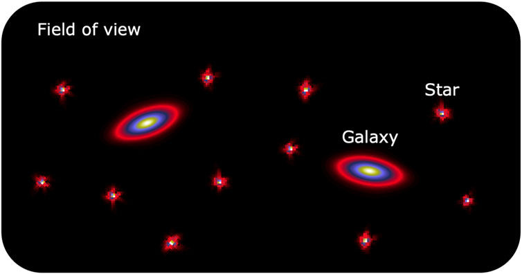
FIGURE 1. Illustration of a field of view showing the PSF modelling problem. Firstly, the PSF model should be estimated from the stars. The model should then be used to estimate the PSF at the target positions, e.g., galaxy positions.

TABLE 1

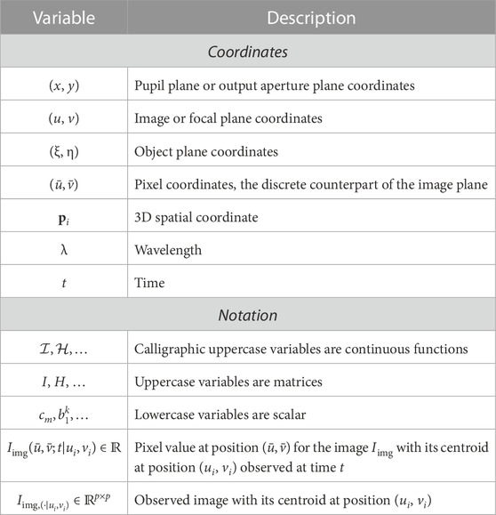
TABLE 1. Coordinates and notation used throughout this article.

2 Gentle introduction to optics

A rigorous treatment of the optics involved in the formation of the PSF on complex optical systems could be the sole topic of a review article. In this section, we introduce simplified optical concepts to motivate a more physical understanding of the PSF, how to model it, and certain implicit assumptions that are usually adopted. This review follows the optic formalism of Goodman (2005). For a profound and rigorous description of optical theory, we refer the readers to the seminal book of Born and Wolf (1999) or more concise works (Gaskill, 1978; Gross, 2005; Hecht, 2017); for more information on practical wave propagation, we refer the readers to Schmidt (2010); and if the readers are familiar with the Fourier optics literature, we recommend continuing to Section 3.

This introduction is based on the scalar formulation of diffraction. It starts by presenting diffraction equations from a general perspective with the Huygens–Fresnel principle to the more simplified formulations of Fresnel and Fraunhofer. The introduction continues with the diffraction analysis of the effects of a thin single-lens optical system. The results motivate the analysis of more general optical systems that are treated with the black box concept from Goodman (2005). The section proceeds by introducing the modelling of aberrations in the optical system, and then extending the monochromatic to the polychromatic analysis briefly studying the coherent and incoherent cases. The optical introduction ends by mentioning several assumptions usually adopted in the PSF modelling literature.

2.1 Scalar diffraction theory

2.1.1 Huygens–Fresnel principle

When studying the PSF, we are examining how an optical system with a specific instrument contributes to and modifies our observations. To understand how the optical system interacts with the propagation of light, we have to dig into the nature of light, an electromagnetic (EM) wave. To make a fundamental analysis, one would have to use Maxwell’s equations, solve them with the optical system under study, and obtain the electric and magnetic fields. Solving a set of coupled partial differential equations is an arduous task. Several approximations can be made, if some conditions are met, to alleviate the mathematical burden of solving Maxwell’s equations without introducing much error into the analysis.

The diffraction theory provides a fundamental framework for analysing light propagation through an optical system. This is especially the case when working with EM waves in the optical range when the optical image is close to the focus region. The Huygens–Fresnel principle (Huygens, 1690; Fresnel, 1819; Crew et al., 1900) states that every point of a wavefront may be considered a secondary disturbance giving rise to spherical wavelets. At any later instant, the wavefront may be regarded as the envelope of all the disturbances. Fresnel’s contribution to the principle is that the secondary wavelets mutually interfere. This principle provides a powerful method of analysis of luminous wave propagation. In Figure 2A, the propagation of an incident plane wavefront through an obstacle, a single slit, is shown. The secondary wavelets constitute the plane wavefront before the obstacle. Then, the wavefront shape is modified due to the obstacle, following the Huygens–Fresnel principle.

FIGURE 2

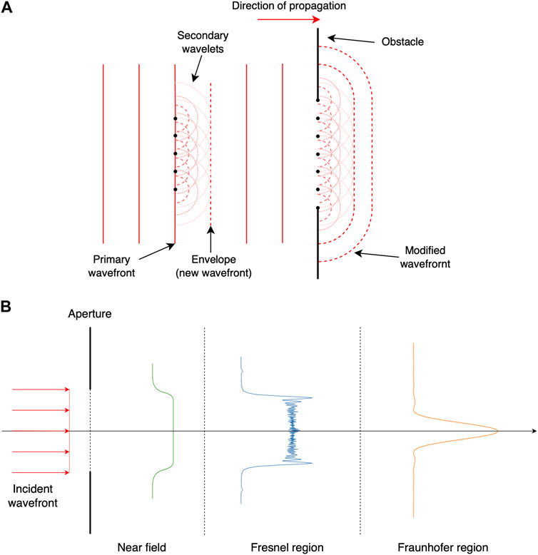
FIGURE 2. (A) Illustration of the Huygens–Fresnel principle and the modification of a wavefront due to an obstacle. Reproduced from Liaudat (2022). (B) Illustration of the different diffraction regions behind an aperture.

The secondary waves mutually interfere constructively or destructively, according to their phases. The analysis of the light propagation in a homogeneous medium is simple as the spherical wavelets interfere without obstacles, and the total wavefront propagates spherically in the medium. However, suppose the wave encounters an obstacle. In that case, the secondary waves in the vicinity of the boundaries of the obstacle will interfere in ways that are not obvious from the incident wavefront.

Let us study the Huygens–Fresnel principle and consider a diffractive aperture in a plane (x, y) illuminated in the positive z direction. We analyse the diffracted wave in a parallel plane (u, v) at a normal distance z from the first plane. The z-axis is orthogonal to both planes and intersects them at their origins. Figure 3 illustrates the coordinate system described previously. The diffracted wave, which can be intuitively understood as the superposition of spherical waves, is written as

$\mathcal{U}\left({\mathbf{p}}_1\right)=\frac{z}{\text{j}\lambda }{\iint }_{\mathrm{\Sigma }}\mathcal{U}\left(x,y;0\right)\frac{\exp \left[\text{j}k{r}_{01}\right]}{r_{01}^2}\mathrm{d}x\mathrm{d}y,(1)$

where j denotes the imaginary unit, λ is the wavelength, k = 2π/λ, p₀ = (x₀, y₀; 0), p₁ = (u₁, v₁; z), r₀₁ = ‖p₁ − p₀‖₂, Σ is the aperture in the (x, y) plane, and $\mathcal{U}$ is the electric field. The incident wave is $\mathcal{U}({\mathbf{p}}_0)$, and the diffracted wave is $\mathcal{U}({\mathbf{p}}_1)$.

FIGURE 3

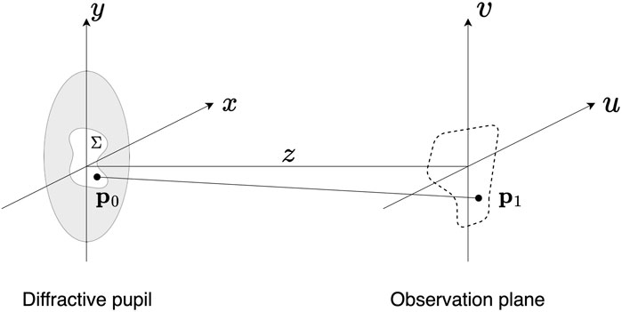
FIGURE 3. Illustration of the coordinate system for the diffraction equations. Figure adapted from Liaudat (2022).

There are two main approximations in the derivation of Eq. 1. The first approximation is that we are considering a scalar theory of diffraction, a scalar electric and magnetic field, and not the fields in their complete vectorial form. The scalar theory provides a full description of the EM fields in a dielectric medium that is linear, isotropic, homogeneous, and non-dispersive. However, even if the medium verifies these properties, when some boundary conditions are imposed on a wave, e.g., an aperture, some coupling is introduced between the EM field components and the scalar theory becomes no longer exact. Nevertheless, the EM fields are modified only at the edges of the aperture, and the effects extend over only a few wavelengths into the aperture. Therefore, if the aperture is large when compared to the wavelength, the error introduced by the scalar theory is negligible. Refractive optical elements can also induce polarisation of the EM field. The level of accuracy desired will determine if the bias introduced can be neglected or has to be taken into account.

Although the current formulation is powerful in representing the diffraction phenomena, it is still challenging to work with the integral from Eq. 1. As a consequence, we will explore further approximations that will give origin to the Fresnel diffraction and Fraunhofer diffraction.

2.1.2 Fresnel diffraction

The Fresnel approximation is based on the binomial expansion of the square root in the expression $\sqrt{1+b}$ for some b¹. The distance r₀₁ can be expressed as

$r_{01}=z\sqrt{1+{\left(\frac{u_1-x_0}{z}\right)}^2+{\left(\frac{v_1-y_0}{z}\right)}^2},(2)$

which can be approximated using the first two terms of the binomial expansion, as

$r_{01}\approx z\left(1+\frac{1}{2}{\left(\frac{u_1-x_0}{z}\right)}^2+\frac{1}{2}{\left(\frac{v_1-y_0}{z}\right)}^2\right).(3)$

The r₀₁ appearing in the exponential of Eq. 1 has much more influence on the result than the $r_{01}^2$ in the divisor. Therefore, we use Eq. 3 to approximate r₀₁ in the exponential, and for the divisor, we approximate $r_{01}^2\approx z^2$. Then, we can express the diffracted field as

$\begin{array}{ll}\hfill \mathcal{U}\left(u_1,v_1;z\right)& =\frac{\exp \left[\text{j}kz\right]}{\text{j}\lambda z}{\iint }_{\mathrm{\Sigma }}\mathcal{U}\left(x,y;0\right)\hfill \\ \hfill & \times \exp \left[\text{j}\frac{k}{2z}\left[{\left(u_1-x\right)}^2+{\left(v_1-y\right)}^2\right]\right]\mathrm{d}x\mathrm{d}y,\hfill \end{array}(4)$

and if we expand the terms in the exponential, we get

$\begin{array}{ll}\hfill \mathcal{U}\left(u_1,v_1;z\right)& =\frac{\exp \left[\text{j}kz\right]}{\text{j}\lambda z}\exp \left[\text{j}\frac{k}{2z}\left(u_1^2+v_1^2\right)\right]\hfill \\ \hfill & \times {\iint }_{\mathrm{\Sigma }}\left\{\mathcal{U}\left(x,y;0\right)\exp \left[\text{j}\frac{k}{2z}\left(x^2+y^2\right)\right]\right\}\hfill \\ \hfill & \times \exp \left[-\text{j}\frac{2\pi }{\lambda z}\left(u_{1}x+v_{1}y\right)\right]\mathrm{d}x\mathrm{d}y.\hfill \end{array}(5)$

The Fourier transform (FT) expression can be recognised with some multiplicative factors in Eq. 5. The diffracted wave is the FT of the product of the incident wave and a quadratic phase exponential. In this case, we have approximated the spherical secondary waves of the Huygens–Fresnel principle by parabolic wavefronts. The approximation in the Fresnel diffraction formula is equivalent to the paraxial approximation Goodman (2005, §4.2.3). This last approximation consists of a small-angle approximation as it restricts the rays to be close to the optical axis. This restriction also allows us to approximate Eq. 2 with Eq. 3. The region where the approximation is valid is known as the region of Fresnel diffraction. In this region, the major contributions to the integral come from points (x, y) for which x ≈ u and y ≈ v, i.e., the higher-order terms in the expansion that we are not considering are unimportant. The region of Fresnel diffraction can be seen as the coordinates (u, v, z) that verify

$z^3\gg \frac{\pi }{4\lambda }{\left({\left(u-x\right)}^2+{\left(v-y\right)}^2\right)}^2,\forall \left(x,y\right)\in \mathrm{\Sigma }.(6)$

A more practical and widely used condition is the Fresnel number (Hecht, 2017, §10.3.3) which can be written as follows:

$N_F=\frac{r^2}{\lambda z},(7)$

where r is the radius of a circular aperture and z is the distance from the aperture. If N_F is close to unity, the Fresnel diffraction is a good approximation. However, if N_F ≪ 1, then Fraunhofer’s approximation, which we will introduce in the following section, is valid. For more information on the validity of the Fresnel approximation, we refer the readers to Southwell (1981) and Rees (1987).

2.1.3 Fraunhofer diffraction

We continue to present a further approximation that, if valid, can significantly simplify the calculations. The Fraunhofer approximation assumes that the exponential term with a quadratic dependence of (x, y) is approximately unity over the aperture. The region where the approximation is valid is the far field or Fraunhofer region. Figure 2B illustrates the different diffraction approximations as a function of the aperture’s distance. The required condition to be in this region reads

$z\gg \frac{k\left(x^2+y^2\right)}{2},\forall \left(x,y\right)\in \mathrm{\Sigma }.(8)$

The Fraunhofer diffraction formula is given by

$\begin{array}{ll}\hfill \mathcal{U}\left(u_1,v_1;z\right)& =\frac{\exp \left[\text{j}kz\right]}{\text{j}\lambda z}\exp \left[\text{j}\frac{k}{2z}\left(u_1^2+v_1^2\right)\right]{\iint }_{\mathrm{\Sigma }}\left\{\mathcal{U}\left(x,y;0\right)\right\}\hfill \\ \hfill & \times \exp \left[-\text{j}\frac{2\pi }{\lambda z}\left(u_{1}x+y{v}_1\right)\right]\mathrm{d}x\mathrm{d}y,\hfill \end{array}(9)$

where we can reformulate the previous equation using the FT as follows:

$\begin{array}{ll}\hfill \mathcal{U}\left(u_1,v_1;z\right)& =\frac{\exp \left[\text{j}kz\right]}{\text{j}\lambda z}\exp \left[\text{j}\frac{k}{2z}\left(u_1^2+v_1^2\right)\right]\hfill \\ \hfill & \times \text{FT}\left\{{ɩ}_{\mathrm{\Sigma }}\left(x,y;0\right)\mathcal{U}\left(x,y;0\right)\right\}\left(\frac{u_1}{\lambda z},\frac{v_1}{\lambda z}\right),\hfill \end{array}(10)$

where ɩ_Σ is an indicator function over the aperture taking values in {0, 1}. It is also possible to consider image vignetting and multiply the indicator with a weight function so that the resulting function takes values in [0, 1]. Cameras are sensitive to the light’s intensity reaching their detectors. The instantaneous intensity of an EM wave is equal to its squared absolute value. Therefore, we can write the intensity of the diffracted wave as

$\begin{array}{ll}\hfill \mathcal{I}\left(u_1,v_1;z\right)& ={\left|\mathcal{U}\left(u_1,v_1;z\right)\right|}^2\hfill \\ \hfill & =\frac{1}{{\lambda }^2{z}^2}{\left|\text{FT}\left\{{ɩ}_{\mathrm{\Sigma }}\left(x,y;0\right)\mathcal{U}\left(x,y;0\right)\right\}\left(\frac{u_1}{\lambda z},\frac{v_1}{\lambda z}\right)\right|}^2,\hfill \end{array}(11)$

which is significantly simpler than the original Rayleigh–Sommerfeld expression from Eq. 1.

2.2 Modelling diffraction in a simple optical system

The study of the diffraction phenomena is necessary but not sufficient to describe the effects of an optical system. Optical imaging systems are generally based on lenses or mirrors, which have the ability to form images. To simplify the analysis, we studied the effect of a single positive (converging) thin lens illuminated with monochromatic illumination and computed the impulse response of such a system. The coordinate system used for this analysis is shown in Figure 4.

FIGURE 4

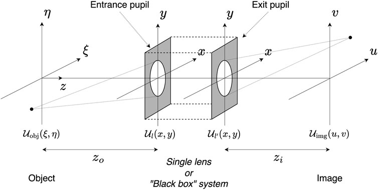
FIGURE 4. Illustration of the coordinate system of the imaging systems we are studying. The central imaging system can be a single positive lens or the generalised black box concept of an imaging system. The image plane coordinates are (u, v), the input and output aperture plane coordinates are (x, y), and the object plane coordinates are (ξ, η). This figure has been adapted from Goodman (2005).

Let us write the output wave as a function of the input wave using the superposition integral as follows:

${\mathcal{U}}_{\text{img}}\left(u,v\right)={\iint }_{-\infty }^{+\infty }\mathcal{H}\left(u,v;\xi ,\eta \right){\mathcal{U}}_{\text{obj}}\left(\xi ,\eta \right)\mathrm{d}\xi \mathrm{d}\eta ,(12)$

where $\mathcal{H}$ is the field’s value at image coordinates (u, v) due to a unitary point-source object at position (ξ, η). We describe a monochromatic input wave reaching the entrance pupil of the lens coming from a point source located at (ξ, η) at the object plane, which is located at a distance z_o from the lens. Following the paraxial approximation, we can write the waves at the entrance pupil as follows:

${\mathcal{U}}_l\left(x,y\right)=\frac{1}{\text{j}\lambda z_o}\exp \left[\text{j}\frac{k}{2z_o}\left({\left(x-\xi \right)}^2+{\left(y-\eta \right)}^2\right)\right],(13)$

and the wave at the output pupil is as follows:

${\mathcal{U}}_{l^{\prime }}\left(x,y\right)={\mathcal{U}}_l\left(x,y\right)\mathcal{P}\left(x,y\right)\exp \left[-\text{j}\frac{k}{2f}\left(x^2+y^2\right)\right],(14)$

where f is the focal length of the lens and $\mathcal{P}$ is the pupil function of the lens which accounts for the finite dimension of the lens, i.e., the obscured and unobscured areas. We have implicitly assumed that the pupil function is constant for any (u, v) position considered. This assumption does not hold for wide-field imagers where there are obscurations involved in the pupil function. We continue by using the Fresnel diffraction formula from Section 2.1.2 to compute the diffraction effect from the lens’ exit pupil to the image plane. Replacing $\mathcal{U}$ in Eq. 5 with the output lens wave ${\mathcal{U}}_{l^{\prime }}$ to compute the impulse response, we obtain

$\begin{array}{ll}\hfill \mathcal{H}\left(u,v;\xi ,\eta \right)& =\frac{1}{{\lambda }^2{z}_o{z}_i}\stackrel{\left(\text{II}\right)}{\overbrace{\exp \left[\text{j}\frac{k}{2z_i}\left(u^2+v^2\right)\right]}}\stackrel{\left(\text{III}\right)}{\overbrace{\exp \left[\text{j}\frac{k}{2z_o}\left({\xi }^2+{\eta }^2\right)\right]}}\hfill \\ \hfill & \times {\iint }_{-\infty }^{\infty }\mathcal{P}\left(x,y\right)\underset{\left(\text{I}\right)}{\underbrace{\exp \left[\text{j}\frac{k}{2}\left(\frac{1}{z_o}+\frac{1}{z_i}-\frac{1}{f}\right)\left(x^2+y^2\right)\right]}}\hfill \\ \hfill & \times \exp \left[-\text{j}k\left(\left(\frac{\xi }{z_o}+\frac{u}{z_i}\right)x+\left(\frac{\eta }{z_o}+\frac{v}{z_i}\right)y\right)\right]\mathrm{d}x\mathrm{d}y.\hfill \end{array}(15)$

The previous formula of the impulse response of a positive lens is hard to exploit in a practical sense due to the quadratic phase terms. However, several approximations can be exploited to remove them.

•We start studying the term (I) inside the integrand. We consider the image plane to coincide with the focal plane, i.e., z_i = f, and the imaged object to be very far away from the entrance pupil. Consequently, the term (I) is approximately one. The part of the exponent which is close to zero is

$\frac{1}{z_o}+\frac{1}{z_i}-\frac{1}{f}\approx 0,(16)$

which, in the case of equality, is known as the lens law of geometrical optics.

•The term (II) only depends on the image coordinates (u, v). The term can be ignored as we are interested in the intensity distribution of the image, and it is not being integrated in Eq. 12.

•The term (III) depends on the object coordinates, is integrated into the convolution operation in Eq. 12, and therefore might significantly change the imaged object. We can neglect the influence of this term if its phase changes by a small amount, i.e., a small fraction of a radian, within the region of the object that mostly contributes to the image position (u, v). A deeper discussion about the validity of the term (III) approximation is found in Goodman (2005, §5.3.2) and references therein.

We can now apply the previous approximations to the calculation of the impulse response of an optical system with a positive lens. Under Fresnel diffraction, we simplify Eq. 15 to obtain

$\begin{array}{ll}\hfill \mathcal{H}\left(u,v;\tilde{\xi },\tilde{\eta }\right)& \approx \frac{1}{{\lambda }^2{z}_{o}f}{\iint }_{-\infty }^{+\infty }\mathcal{P}\left(x,y\right)\hfill \\ \hfill & \times \exp \left[-\text{j}\frac{2\pi }{\lambda f}\left(\left(u-\tilde{\xi }\right)x+\left(v-\tilde{\eta }\right)y\right)\right]\mathrm{d}x\mathrm{d}y,\hfill \end{array}(17)$

where m = −f/z_o is the magnification of the system, which can be positive or negative depending on whether the image is inverted or not, and the normalised (or reduced) object-plane coordinates are $\tilde{\xi }=m\xi$ and $\tilde{\eta }=m\eta$. The diffraction pattern is centred on the image coordinates, u = m ξ and v = m η, which are the transformed coordinates of the impulse response’s position (ξ, η).

The impulse response obtained in Eq. 17 is Fraunhofer’s diffraction pattern centred in $(u=\tilde{\xi },v=\tilde{\eta })$ and up to a scaling factor of 1/λz_o. This result is the consequence of the choice of z_i, such that it verifies the lens law, allowing us to drop out quadratic phase terms in the integral. We have obtained a simple formulation for the impulse response, but the optical system that we studied is not used in practice to carry out galaxy imaging surveys. We have to extend the analysis to more general optical systems.

2.3 Analysis of a general optical imaging system

Let us now analyse a general optical imaging system composed of one or many lenses or mirrors of possibly different characteristics. We treat the optical system as a black box characterised by the transformations applied to an incident object scalar wave, ${\mathcal{U}}_{\text{obj}}$, into an output image wave, ${\mathcal{U}}_{\text{img}}$. Figure 4 illustrates the new interpretation of the optical system, where we have replaced the previous single-lens system with a black box. In this general model, we assume that the effect of the optical system between the entrance and exit pupils is well described by geometrical optics, which is an affine transformation. We also assume that all the diffraction effects can be associated with one of the two pupils, input or output (for more discussion on both assumptions, see Goodman, 2005, §6.1). We choose the latter and consider the diffraction of the output wave between the output pupil and image plane. For the moment, our analysis continues to assume an ideal monochromatic illumination.

The ideal image, ${\mathcal{U}}_{\mathrm{g}}$, is defined as the input image when applying the effect of geometrical optics inside the black box and is given as

${\mathcal{U}}_{\mathrm{g}}\left(\tilde{\xi },\tilde{\eta }\right)=\frac{1}{|m|}{\mathcal{U}}_{\text{obj}}\left(\frac{\tilde{\xi }}{m},\frac{\tilde{\eta }}{m}\right),\text{and}\tilde{\xi }=m\xi ,\tilde{\eta }=m\eta ,(18)$

where m is the magnification factor of the optical system, and we express the images in reduced coordinates.

Our analysis is based on the impulse response developed in the previous section. The approximations applied and the use of reduced object coordinates have made the system spatially invariant. This fact translates to having $\mathcal{H}(u,v;\tilde{\xi },\tilde{\eta })=\mathcal{H}(u-\tilde{\xi },v-\tilde{\eta })$, as the approximated impulse response from Eq. 17 depends only on the difference of the image coordinates and the reduced object coordinates. The impulse response is given as

$\begin{array}{ll}\hfill \mathcal{H}\left(u-\tilde{\xi },v-\tilde{\eta }\right)& =\frac{a}{\lambda f}{\iint }_{-\infty }^{+\infty }\mathcal{P}\left(x,y\right)\hfill \\ \hfill & \times \exp \left[-\text{j}\frac{2\pi }{\lambda f}\left(\left(u-\tilde{\xi }\right)x+\left(v-\tilde{\eta }\right)y\right)\right]\mathrm{d}x\mathrm{d}y,\hfill \end{array}(19)$

where a is a constant amplitude that does not depend on the optical system under study. The superposition integral in Eq. 12 relates the waves at the object and image positions with the impulse response in a spatially variant system. However, if the system is spatially invariant, the equation can be reformulated as the convolution equation, which is given as

${\mathcal{U}}_{\text{img}}\left(u,v\right)={\iint }_{-\infty }^{+\infty }\mathcal{H}\left(u-\tilde{\xi },v-\tilde{\eta }\right){\mathcal{U}}_{\mathrm{g}}\left(\tilde{\xi },\tilde{\eta }\right)\mathrm{d}\tilde{\xi }\mathrm{d}\tilde{\eta }.(20)$

The previous equation can be rewritten with the usual convolution notation as

${\mathcal{U}}_{\text{img}}\left(u,v\right)=\left({\mathcal{U}}_{\mathrm{g}}\star \mathcal{H}\right)\left(u,v\right).(21)$

In this general case of a system without aberrations and under the aforementioned approximations, we see that the output image is formed by a geometrical-optics transformation followed by a convolution with an impulse response from the Fresnel diffraction of the exit aperture.

2.3.1 Introducing optical aberrations

In the previous development, we considered an ideal optical system without any aberrations, known as diffraction-limited. An aberrated optical system produces the imperfect convergence of rays, which can be expressed equivalently in wavefront space by deviations from the ideal reference sphere. The aberrations produce leads and lags in the wavefront with respect to the ideal sphere (see Figure 5). A complementary interpretation, from Goodman (2005), is that we start with the previous diffraction-limited system producing converging spherical wavefronts. Then, we add a phase-shifting plate representing the system’s aberrations. The plate is located at the aperture after the exit pupil and affects the output wave’s phase. To characterise the aberrations, we use the generalised pupil function that generalises the pupil function $\mathcal{P}$ from Eq. 19 and gives

${\mathcal{P}}_{\text{gen}}\left(x,y;u,v\right)=\mathcal{P}\left(x,y;u,v\right)\exp \left[\text{j}\frac{2\pi }{\lambda }\mathcal{W}\left(x,y;u,v\right)\right],(22)$

where λ is the central wavelength of the incident wave, $\mathcal{P}$ is the pupil function that includes the telescope’s obscurations, and $\mathcal{W}$ represents the optical path differences (OPDs) between a perfectly spherical and the aberrated wavefront. We also refer to the OPD as the wavefront error (WFE). Figure 5 illustrates the concept of WFE. It is common to represent the WFE using a Zernike polynomial decomposition (Noll, 1976) as these are orthogonal in the unit disk, and we generally use circular apertures in telescopes and optical systems. Figure 6B shows the first Zernike polynomials.

FIGURE 5

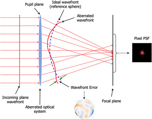
FIGURE 5. Illustration of the wavefront error in a one-dimensional projection of an ideal setting where the optical system is represented as a single lens. Figure reproduced from Liaudat et al. (2023).

FIGURE 6

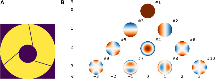
FIGURE 6. (A) Illustration of Euclid’s pupil function, which can be seen in Venancio et al. (2020), in the (x, y) plane for a given position in the (ξ, η). (B) Example of the first Zernike polynomial maps.

The aberrations, $\mathcal{W}$, and pupil function, $\mathcal{P}$, depend on the object’s position in the focal plane as is seen in the (u, v) coordinate dependence in Eq. 22. Large telescopes with wide focal planes have spatially varying aberrations. The path travelled by the light rays changes considerably between distant points in the focal plane, also changing the aberrations, $\mathcal{W}$. The obscurations and aperture, represented by the pupil function $\mathcal{P}$, also change with the focal plane position. For example, Figure 6A illustrates the obscurations from the Euclid telescope. One can notice a circular aperture with several obscurations in it, a secondary mirror, and three arms supporting the mirror. What we observe in Figure 6A is a 2D projection of the 3D structure. This projection changes as a function of the focal plane position that we are analysing, making the function $\mathcal{P}$ dependent on the (u, v) coordinates.

In the impulse response of the optical system without aberrations from Eq. 19, we had a spatially invariant system. This invariance allowed us to use the convolution rather than the superposition integral, which is a computationally practical formulation. If we now consider aberrations, we must inject the generalised pupil function appearing in Eq. 22 into the impulse response formula from Eq. 19. The addition of the (u, v) dependency in ${\mathcal{P}}_{\text{gen}}$ makes the impulse response $\mathcal{H}$ spatially variant again.

The study of $\mathcal{H}$, the impulse response and the main topic of this review, is strongly spatially variant in systems with a large focal plane. Nevertheless, we can consider $\mathcal{H}$ spatially invariant in its isoplanatic region. This region consists of close-by points in the focal plane, where the light has travelled similar paths giving small deviations of $\mathcal{H}$. We are assuming a certain regularity in $\mathcal{H}$ due to the optical system under study that allows the deviations to be small. In other words, we consider $\mathcal{H}$ to be locally spatially invariant or spatially invariant in patches. Figure 7 illustrates the idea of an isoplanatic region. This local invariance assumption limits the size of the imaged objects under study, as they should have a certain size range with respect to the support of $\mathcal{H}$ so that all the objects being imaged lie within the aforementioned region. We consider the generalised pupil function evaluated at the centroid of the imaged object, (u_i, v_i), and note the locally spatially invariant generalised pupil function as follows:

${\mathcal{P}}_{\text{gen}}^{*}\left(x,y|u_i,v_i\right)={\mathcal{P}}^{*}\left(x,y|u_i,v_i\right)\exp \left[\text{j}\frac{2\pi }{\lambda }{\mathcal{W}}^{*}\left(x,y|u_i,v_i\right)\right].(23)$

Injecting Eq. 23, instead of Eq. 22, to the impulse response in Eq. 19 gives

$\begin{array}{ll}\hfill \mathcal{H}\left(u-\tilde{\xi },v-\tilde{\eta }|u_i,v_i\right)& =\frac{a}{\lambda f}{\iint }_{-\infty }^{+\infty }{\mathcal{P}}^{*}\left(x,y|u_i,v_i\right)\hfill \\ \hfill & \times \exp \left[\text{j}\frac{2\pi }{\lambda }{\mathcal{W}}^{*}\left(x,y|u_i,v_i\right)\right]\exp \hfill \\ \hfill & \times \left[-\text{j}\frac{2\pi }{\lambda f}\left(\left(u-\tilde{\xi }\right)x+\left(v-\tilde{\eta }\right)y\right)\right]\mathrm{d}x\mathrm{d}y,\hfill \end{array}(24)$

where we have made the system spatially invariant again, allowing us to exploit the convolution formula in Eq. 20.

FIGURE 7

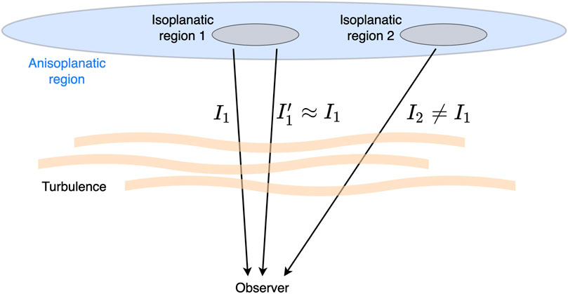
FIGURE 7. Illustration of isoplanatic regions. Two rays from the same isoplanatic region travel through almost the same turbulence and suffer almost the same distortions. Figure reproduced from Liaudat (2022).

We have considered aberrations that only depend on the object’s position in the focal plane, also known as achromatic aberrations. However, depending on the optical system under study, there might be wavelength-dependent aberrations. For example, some refractive components, or some components implementing complex thin film coatings, may introduce spurious spectral dependences to the optical system’s response. If this is the case, we can add a wavelength dependence to the WFE function $\mathcal{W}$ to account for these effects.

2.3.2 Polychromatic illumination: coherent and incoherent cases

We studied until now a system with ideal monochromatic light. It is time to shift to polychromatic light as telescopes have filters with finite bandwidths and hence allow multiple frequencies of light. For a more rigorous analysis of polychromatic illumination, we refer the readers to the theory of partial coherence in Beran and Parrent (1964), Goodman (1985), and Born and Wolf (1999, §10). Even if we were to study the system’s behaviour to light with a particular wavelength, this has practically never been the case, as real illumination is never perfectly chromatic, even for lasers. Therefore, we consider a narrowband polychromatic illumination centred at a given wavelength λ. The narrowband assumption states that the bandwidth occupied is small with respect to the central wavelength. For polychromatic light, we follow Goodman (2005) and consider a time-varying phasor of the field, ${\mathcal{U}}_{\text{img}}(u,v;t)$, where its intensity is given by the time integration of its instantaneous intensity:

${\mathcal{I}}_{\text{img}}\left(u,v\right)={⟨{\left|{\mathcal{U}}_{\text{img}}\left(u,v;t\right)\right|}^2⟩}_t=\frac{1}{T}{\int }_{-T/2}^{T/2}{\left|{\mathcal{U}}_{\text{img}}\left(u,v;t\right)\right|}^2\mathrm{d}t,(25)$

where T is the detector integration time that is considered to be much greater than the optical wave period. We can generalise the field expression from Eq. 20 by considering that light is polychromatic and that the impulse response $\mathcal{H}$ is wavelength independent due to the narrowband assumption. The field then is given as

${\mathcal{U}}_{\text{img}}\left(u,v;t\right)={\iint }_{-\infty }^{+\infty }\mathcal{H}\left(u-\tilde{\xi },v-\tilde{\eta }\right){\mathcal{U}}_{\mathrm{g}}\left(\tilde{\xi },\tilde{\eta };t-\tau \right)\mathrm{d}\tilde{\xi }\mathrm{d}\tilde{\eta },(26)$

where τ represents the delay of the wave propagation from $(\tilde{\xi },\tilde{\eta })$ to (u, v). Continuing with the polychromatic analysis, we rewrite the intensity from Eq. 25 as

$\begin{array}{ll}\hfill {\mathcal{I}}_{\text{img}}\left(u,v\right)& =\underset{-\infty }{\overset{+\infty }{\iint }}\mathrm{d}{\tilde{\xi }}_1\mathrm{d}{\tilde{\eta }}_1\underset{-\infty }{\overset{+\infty }{\iint }}\mathrm{d}{\tilde{\xi }}_2\mathrm{d}{\tilde{\eta }}_2\mathcal{H}\left(u-{\tilde{\xi }}_1,v-{\tilde{\eta }}_1\right)\hfill \\ \hfill & \times {\mathcal{H}}^{*}\left(u-{\tilde{\xi }}_2,v-{\tilde{\eta }}_2\right){\mathcal{J}}_{\mathrm{g}}\left({\tilde{\xi }}_1,{\tilde{\eta }}_1;{\tilde{\xi }}_2,{\tilde{\eta }}_2\right),\hfill \end{array}(27)$

where ${\mathcal{H}}^{*}$ is the conjugate of $\mathcal{H}$, ${\mathcal{J}}_{\mathrm{g}}$ is known as the mutual intensity which describes the spatial coherence of ${\mathcal{U}}_{\mathrm{g}}$ at two points and is given as

${\mathcal{J}}_{\mathrm{g}}\left({\tilde{\xi }}_1,{\tilde{\eta }}_1;{\tilde{\xi }}_2,{\tilde{\eta }}_2\right)=⟨{\mathcal{U}}_{\mathrm{g}}\left({\tilde{\xi }}_1,{\tilde{\eta }}_1;t\right){\mathcal{U}}_{\mathrm{g}}^{*}\left({\tilde{\xi }}_2,{\tilde{\eta }}_2;t\right)⟩.(28)$

We can distinguish two types of illuminations, coherent and incoherent. Coherent illumination refers to waves whose phases vary in a perfectly correlated way. This illumination is approximately the case of a laser. In incoherent illumination, the wave’s phases vary in an uncorrelated fashion. Most natural light sources can be considered incoherent sources. The mutual intensity is helpful to represent both types of illumination. In the case of coherent light, we obtain

${\mathcal{J}}_{\mathrm{g}}^{\text{co}}\left({\tilde{\xi }}_1,{\tilde{\eta }}_1;{\tilde{\xi }}_2,{\tilde{\eta }}_2\right)={\mathcal{U}}_{\mathrm{g}}\left({\tilde{\xi }}_1,{\tilde{\eta }}_1\right){\mathcal{U}}_{\mathrm{g}}^{*}\left({\tilde{\xi }}_2,{\tilde{\eta }}_2\right),(29)$

where ${\mathcal{U}}_{\mathrm{g}}\left({\tilde{\xi }}_1,{\tilde{\eta }}_1\right)$ and ${\mathcal{U}}_{\mathrm{g}}^{*}\left({\tilde{\xi }}_2,{\tilde{\eta }}_2\right)$ are time-independent phasor amplitudes relative to their time-varying counterpart. As both time-varying phasors are synchronized, we have taken a reference phasor and normalised it against the amplitude with respect to a reference point that can be the origin (0, 0). For example,

${\mathcal{U}}_{\mathrm{g}}\left({\tilde{\xi }}_1,{\tilde{\eta }}_1;t\right)={\mathcal{U}}_{\mathrm{g}}\left({\tilde{\xi }}_1,{\tilde{\eta }}_1\right)\frac{{\mathcal{U}}_{\mathrm{g}}\left(\mathrm{0,0};t\right)}{{⟨{\left|{\mathcal{U}}_{\mathrm{g}}\left(\mathrm{0,0};t\right)\right|}^2⟩}^{\frac{1}{2}}}.(30)$

By substituting Eq. 29 in Eq. 27, we obtain

$\begin{array}{ll}\hfill {\mathcal{I}}_{\text{img}}^{\text{co}}\left(u,v\right)& ={\left|{\mathcal{U}}_{\text{img}}^{\text{co}}\left(u,v\right)\right|}^2\hfill \\ \hfill & ={\left|{\iint }_{-\infty }^{+\infty }\mathcal{H}\left(u-\tilde{\xi },v-\tilde{\eta }\right){\mathcal{U}}_{\mathrm{g}}\left(\tilde{\xi },\tilde{\eta }\right)\mathrm{d}\tilde{\xi }\mathrm{d}\tilde{\eta }\right|}^2,\hfill \\ \hfill {\mathcal{I}}_{\text{img}}^{\text{co}}\left(u,v\right)& ={\left|\left({\mathcal{U}}_{\mathrm{g}}\star \mathcal{H}\right)\left(u,v\right)\right|}^2,\hfill \end{array}(31)$

where we observe that the coherent illumination gives a linear system in the complex amplitude of the field ${\mathcal{U}}_{\mathrm{g}}$. The previous result is related to the interference of coherent waves. If we now consider incoherent illumination, the mutual intensity is given by

${\mathcal{J}}_{\mathrm{g}}^{\text{in}}\left({\tilde{\xi }}_1,{\tilde{\eta }}_1;{\tilde{\xi }}_2,{\tilde{\eta }}_2\right)=\kappa {\mathcal{I}}_g\left({\tilde{\xi }}_1,{\tilde{\eta }}_1\right)\delta \left({\tilde{\xi }}_1-{\tilde{\xi }}_2,{\tilde{\eta }}_1-{\tilde{\eta }}_2\right),(32)$

where κ is a real constant, δ is the Dirac delta distribution, and ${\mathcal{I}}_{\mathrm{g}}$ is the intensity of the U_g field. The constant κ is the result of a simplification from statistical optics giving origin to Eq. 32. The constant depends on the degree of the extension of coherence when the evanescent wave phenomenon (Beran and Parrent, 1964) is taken fully into account. If the coherence extends over a wavelength, κ is equal to ${\bar{\lambda }}^2/\pi$, where $\bar{\lambda }$ is the mean wavelength (for a deeper discussion on incoherent illumination and the κ constant, see Goodman, 1985, §5.5.2). By replacing Eq. 32 in Eq. 27, the output (image) intensity obtained is

$\begin{array}{ll}\hfill {\mathcal{I}}_{\text{img}}^{\text{in}}\left(u,v\right)& ={\left|{\mathcal{U}}_{\text{img}}^{\text{in}}\left(u,v\right)\right|}^2\hfill \\ \hfill & =\kappa {\iint }_{-\infty }^{+\infty }{\left|\mathcal{H}\left(u-\tilde{\xi },v-\tilde{\eta }\right)\right|}^2{\mathcal{I}}_{\mathrm{g}}\left(\tilde{\xi },\tilde{\eta }\right)\mathrm{d}\tilde{\xi }\mathrm{d}\tilde{\eta },\hfill \\ \hfill {\mathcal{I}}_{\text{img}}^{\text{in}}\left(u,v\right)& =\kappa \left({\mathcal{I}}_{\mathrm{g}}\star {\left|\mathcal{H}\right|}^2\right)\left(u,v\right)=\kappa \left({\mathcal{I}}_{\mathrm{g}}\star {\mathcal{H}}_{\text{int}}\right)\left(u,v\right),\hfill \end{array}(33)$

where ${\mathcal{H}}_{\text{int}}={\left|\mathcal{H}\right|}^2$ is the intensity impulse response, also known as the PSF. In this case, an optical system illuminated with incoherent light is linear in intensity. Eq. 33 shows a commonly exploited fact; the output intensity is the convolution of the intensity PSF with ideal image intensity ${\mathcal{I}}_{\mathrm{g}}$.

2.4 Usual assumptions adopted in PSF modelling

PSF modelling articles generally implicitly assume specific hypotheses. We provide some of them in the following list:

•The scalar diffraction theory is valid.

•The lens law is verified, the paraxial approximation is valid, and the approximations discussed in Section 2.2 hold. These approximations allow us to discard quadratic phase terms from Fresnel’s diffraction and exploit the simpler Fraunhofer diffraction formula.

•The incoming light from natural sources is assumed to be ideally incoherent. Then, the optical system is linear in intensity, as seen in Eq. 33.

•The PSF is considered to be spatially invariant in its isoplanatic region. In other words, the PSF is assumed not to change on the objects’ typical length scales. This assumption allows us to use the convolution equation, i.e., Eq. 33, rather than the superposition integral, i.e., Eq. 12.

Although the previous assumptions are standard, certain precision levels require dropping simplifications. For example, the Euclid mission requirements on the PSF model accuracy as given in Laureijs et al. (2011) and Racca et al. (2016) is of 2 × 10⁻⁴ for the root mean square (RMS) error on each ellipticity component $(\delta e_i^{\text{PSF}})$ and 1 × 10⁻³ for the relative RMS error on the size $(\delta R_{\text{PSF}}^2/R_{\text{PSF}}^2)$. The PSF model might have to include light polarisation to fulfil these extremely tight PSF requirements. Other assumptions might also be dropped for the precise imaging of widespread objects. This case might require discarding the spatially invariant assumption of the PSF or reducing the size of the isoplanatic region.

To conclude, the usual formulation of the PSF, i.e., the intensity of the impulse response, convolving an image seen in many articles, comes from the previous assumptions using the results from Eqs 23, 24, and 33. We rewrite this formula as follows:

${\mathcal{I}}_{\text{img}}\left(u,v\right)=\left({\mathcal{H}}_{\text{int}}\star {\mathcal{I}}_g\right)\left(u,v\right),(34)$

where we remind the readers that (u, v) is the image plane, we have dropped the κ term from Eq. 33, and ${\mathcal{H}}_{\text{int}}$ is the intensity impulse response or PSF that is given as

$\begin{array}{ll}\hfill {\mathcal{H}}_{\text{int}}\left(u,v|u_i,v_i\right)& =\left.\frac{{a^{\prime }}^2}{{\lambda }^2{f}^2}\right|{\iint }_{-\infty }^{+\infty }{\mathcal{P}}^{*}\left(x,y|u_i,v_i\right)\hfill \\ \hfill & \times \exp \left[\text{j}\frac{2\pi }{\lambda }{\mathcal{W}}^{*}\left(x,y|u_i,v_i\right)\right]\hfill \\ \hfill & \times \exp {\left.\left[-\text{j}\frac{2\pi }{\lambda f}\left(ux+vy\right)\right]\mathrm{d}x\mathrm{d}y\right|}^2,\hfill \end{array}(35)$

where we are studying the PSF for a specific wavelength and focal plane position.

3 General observational model

We consider the PSF as the intensity impulse response, ${\mathcal{H}}_{\text{int}}$, of the imaging system under study to a point source. The concept of PSF (Born and Wolf, 1999) is used throughout many imaging applications, such as astronomical imaging (Schmitz, 2019; Liaudat et al., 2023), medical imaging (Dougherty and Kawaf, 2001; Joyce et al., 2018), or microscopy (Soulez et al., 2012; Debarnot et al., 2021a; Debarnot et al., 2021b). The central idea behind a PSF is that it represents transformations done to the imaged object by the imaging system. The PSF is, in a certain way, a characterisation of the imaging system. Considering incoherent illumination and what the hypotheses from the previous section hold, we can affirm that the optical system behaves linearly as in Eq. 34. Consequently, the PSF is considered the impulse response of the optical system and affects the ground truth image through a convolution operation. Focusing on astronomical imaging, the definition of the imaging system can vary between the different use cases and telescopes. For example, in a ground-based telescope, we will consider that the atmosphere belongs to the imaging system we are modelling. However, naturally, the atmosphere will not be considered in a space-based telescope. This article focuses on optical systems, which work with electromagnetic radiation with a wavelength close to the visible spectrum. For example, Euclid VIS instrument’s theoretical wavelength range is from 550 to 900 nm.

The PSF describes the effects of the imaging system in the imaging process of the object of interest. The PSF is a convolutional kernel, as we have seen in Section 2.3. However, this convolutional kernel varies spatially, spectrally, and temporally. We give a non-exhaustive list that motivates each of these variations.

•Spatial variations: The optical system presents a certain optical axis, which is an imaginary line where the system has some degree of rotational symmetry. In simpler words, it can be considered as the direction of the light ray that produces a PSF in the centre of the focal plane for an unaberrated optical system. The angle of incidence is defined as the angle between an incoming light ray and the optical axis. The main objective of the optical systems that we study is to make the incoming light rays converge in the focal plane, where there will be some measurement instruments, e.g., a camera. Depending on the angle of incidence, the image will form in different positions in the focal plane. The path of the incoming light will be different for each angle of incidence, and therefore the system’s response will be different too. In other words, the PSF will change depending on the angle of incidence or spatial position in the focal plane where the image is forming. Optical systems with wide focal planes, generally associated with wide field-of-views (FOVs), present significant PSF spatial variations.

•Spectral variations: Principally, due to the diffraction phenomena and its well-known wavelength dependence covered in Section 2, refractive² components of the optical system under study are also a source of spectral variations (Baron et al., 2022). Other sources of spectral variations are detector electronic components (Meyers and Burchat, 2015a) and atmospheric chromatic effects (Meyers and Burchat, 2015b).

•Temporal variations: The state of the telescope changes with respect to time, therefore the imaged object’s transformation also changes. In space-based telescopes, high-temperature gradients cause mechanical dilations and contractions that affect the optical system. In ground-based telescopes, the atmosphere composition changes with time. Consequently, it temporally affects the response of the optical system, i.e., the PSF.

The PSF convolutional kernel varies with space, time, and wavelength. Once we have set up a specific wavelength and time to analyse our system, we will have a different convolutional kernel for each position in the field of view. Let us refer to the PSF field ${\mathcal{H}}_{\text{int}}$ as all the PSF representing an optical system. Then, ${\mathcal{H}}_{\text{int}}(u,v;\lambda ;t|u_i,v_i)$ is a specific PSF where (u_i, v_i) represents its centroid, i.e., the first-order moments. The same notation is maintained in Figure 4, where the (u, v) variables represent the image plane. We can define the PSF field as a varying convolutional kernel ${\mathcal{H}}_{\text{int}}:{\mathbb{R}}^2\times {\mathbb{R}}_{+}\times {\mathbb{R}}_{+}\times {\mathbb{R}}^2\to \mathbb{R}$. This definition would accurately describe how the PSF affects the images considering the assumptions from Section 2 are valid. We recall that we adopted the approximation that considers the PSF locally invariant in its isoplanatic region (Born and Wolf, 1999, §9.5.1); for an illustration, see Figure 7. This approximation means that in the vicinity of an observed object, we will consider that the PSF only varies with time and wavelength, thus facilitating the computation of the convolution. The close vicinity, or the isoplanatic region, will be defined as the postage stamp to image the object of interest. The typical galaxies observed for weak lensing have a comparable size with respect to the PSF size (for distribution of the relative galaxy to PSF size in the HSC survey, see Mandelbaum et al., 2018, Figure 7). Consequently, the approximation error is kept low as it is only done for small patches of the focal plane.

Let us define our object of interest with the subscript ground truth (GT), ${\mathcal{I}}_{\text{GT}}(u,v;\lambda ;t|u_i,v_i)$, that is, the I_g object from Section 2, as a continuous light distribution ${\mathcal{I}}_{\text{GT}}:{\mathbb{R}}^2\times {\mathbb{R}}_{+}\times {\mathbb{R}}_{+}\times {\mathbb{R}}^2\to \mathbb{R}$. In this review, we are not considering transient objects, i.e., the time-dependence scale of the object is comparable with the exposure time used to image it. Therefore, we can ignore the temporal dependency of the GT object, ${\mathcal{I}}_{\text{GT}}(u,v;\lambda ;t)\ne f(t)$. Let us write our general observational model that relates our GT object of interest, our PSF, and our observed image as follows:

$\begin{array}{ll}\hfill I_{\text{img}}\left(\bar{u},\bar{v};t|u_i,v_i\right)& ={\mathcal{F}}_p\left\{{\int }_0^{+\infty }\mathcal{T}\left(\lambda \right)\left({\mathcal{I}}_{\text{GT}}\star {\mathcal{H}}_{\text{int}}\right)\left(u,v;\lambda ;t|u_i,v_i\right)\mathrm{d}\lambda \right\}\hfill \\ \hfill & ◦N\left(\bar{u},\bar{v};t|u_i,v_i\right),\hfill \end{array}(36)$

where ${\mathcal{F}}_p$ is a degradation operator discretising the image to ${\mathbb{R}}^{p\times p}$ that includes the image sampling from the instrument. The variables $(\bar{u},\bar{v})$ denote the discrete (pixelised) version of the (u, v) variables. Then, $I_{\text{img}}(\bar{u},\bar{v};t|u_i,v_i)\in \mathbb{R}$ corresponds to the instrument’s measurement at a single pixel $(\bar{u},\bar{v})$, and $I_{\text{img},(\cdot ;t|u_i,v_i)}\in {\mathbb{R}}^{p\times p}$ to the entire image. The variables (u_i, v_i) correspond to the centre location of the target object i. The instrument’s transmission is represented by $\mathcal{T}:{\mathbb{R}}_{+}\to {\mathbb{R}}_{+}$, a function with finite support, and $N_{(\cdot ;t|u_i,v_i)}\in {\mathbb{R}}^{p\times p}$ corresponds to the noise affecting our observation and possibly a modelling error, where ◦ is some composition operator. We have carried out the spectral integration (Hopkins, 1957; Eriksen and Hoekstra, 2018) on the instrument’s passband defined in τ. Although Eq. 36 provides a general observational model, it can be unpractical. The continuous functions ${\mathcal{H}}_{\text{int}}$, $\mathcal{T}$, and ${\mathcal{I}}_{\text{G}T}$ are practically inaccessible. We make several assumptions to simplify the problem.

(a) The continuous functions ${\mathcal{H}}_{\text{int}}$ and ${\mathcal{I}}_{\text{G}T}$ are well approximated by piece-wise constant functions over a regular grid in ${\mathbb{R}}^2$. We assume ${\mathcal{H}}_{\text{int}}\approx H$ and ${\mathcal{I}}_{\text{G}T}\approx I_{\text{G}T}$, where $H,I_{\text{G}T}\in {\mathbb{R}}^{P\times P}$ with P ≥ p. The resolution of these two variables has to be greater or equal to the observation resolution.

(b) The noise is additive, i.e., ◦ ≡ +, although the formulation could be adapted to consider other types of noise, e.g., Poisson.

(c) The degradation operator is approximated by its discrete counterpart, ${\mathcal{F}}_p\approx F_p$, where $F_p:{\mathbb{R}}^{P\times P}\to {\mathbb{R}}^{p\times p}$, which has been discretized in a regular grid. We assume that the degradation operator is linear and that includes pixellation, possibly downsampling, intra-pixel shifts, and linear detector effects.

(d) We keep the approximation that the PSF is locally constant within the postage stamp of P × P values of the target image.

(e) The integral can be well approximated by a discretised version using n_λ bins.

Taking into account the aforementioned assumptions, we can define our practical observational model as follows:

$\begin{array}{ll}\hfill I_{\text{img}}\left(\bar{u},\bar{v};t|u_i,v_i\right)& =F_p\left\{\sum _{k=1}^{n_{\lambda }}T\left({\lambda }_k\right)\left(I_{\text{GT}}\star H\right)\left(\bar{u},\bar{v};{\lambda }_k;t|u_i,v_i\right)\mathrm{\Delta }{\lambda }_k\right\}\hfill \\ \hfill & +N\left(\bar{u},\bar{v};t|u_i,v_i\right),\hfill \end{array}(37)$

where $I_{\text{img},(\cdot ;t|u_i,v_i)}\in {\mathbb{R}}^{p\times p}$, T is a discretized version of $\mathcal{T}$, and $b^k=[b_0^k,b_1^k]$ is the kth wavelength bin centred in λ_k, with a width of $\mathrm{\Delta }{\lambda }_k=b_1^k-b_0^k$.

3.1 Particular case: star observation

The case of star observations is of particular interest, as some stars in the FOV can be considered as a spatial impulse, i.e., ${\mathcal{I}}_{\text{star}}(u,v;\lambda |u_i,v_i)=\delta (u_i,v_i;\lambda )=f_{(u_i,v_i)}(\lambda )$. Therefore, if we plug the impulse in Eq. 37, we obtain a degraded observation of the PSF field. These observations will be crucial to constrain the PSF models. Unluckily, we do not always have access to the star’s spectral variation, $f_{(u_i,v_i)}(\lambda )$. However, we dispose of complementary photometric observations that can be useful to characterise the spectral variations. These observations provide us with the star’s spectral energy distribution (SED), which can be defined as the calibrated flux density as a function of wavelength, usually at low spectral resolution. The photometric observations are done in several spectral bands. Figure 8 shows the bands from the MegaCam instrument at the Canada–France–Hawaii Telescope (CFHT)³. For more information about SEDs and stellar photometry, we refer the readers to Hogg (2022). The SED is a normalised low-resolution sampling of the star’s spectral variations. We can write the SED definition we will use as

${\text{SED}}_{b^k}\left({\lambda }_k\right)=\frac{1}{z_{n_{\lambda }\left(b\right)}}{\int }_{b_0^k}^{b_1^k}{f}_{\left(u_i,v_i\right)}\left(\lambda \right)\mathrm{d}\lambda ,(38)$

where we continued to use the b^k bin definition from Eq. 37, and $z_{n_{\lambda }(b)}$ is a constant used so that the SED is normalised to unity. We have that ${\sum }_{k=1}^{n_{\lambda }}{\text{SED}}_{b^k}({\lambda }_k)=1$, we continue by considering that the GT image in Eq. 37 is a star, and we use the spectral bins from the SED definition to discretise the spectral integration. Finally, we write the practical star observation model as

$\begin{array}{ll}\hfill I_{\text{star}}\left(\bar{u},\bar{v};t|u_i,v_i\right)& =F_p\left\{\sum _{k=1}^{n_{\lambda }}T\left({\lambda }_k\right){\text{SED}}_{b^k}\left({\lambda }_k\right)H\left(\bar{u},\bar{v};{\lambda }_k;t|u_i,v_i\right)\mathrm{\Delta }{\lambda }_k\right\}\hfill \\ \hfill & +N\left(\bar{u},\bar{v};t|u_i,v_i\right),\hfill \end{array}(39)$

where we consider the star observation $I_{\text{star},(\cdot ;t|u_i,v_i)}\in {\mathbb{R}}^{p\times p}$ as a degraded version of the PSF field ${\tilde{H}}_{(\cdot ;t|u_i,v_i)}\in {\mathbb{R}}^{p\times p}$.

FIGURE 8

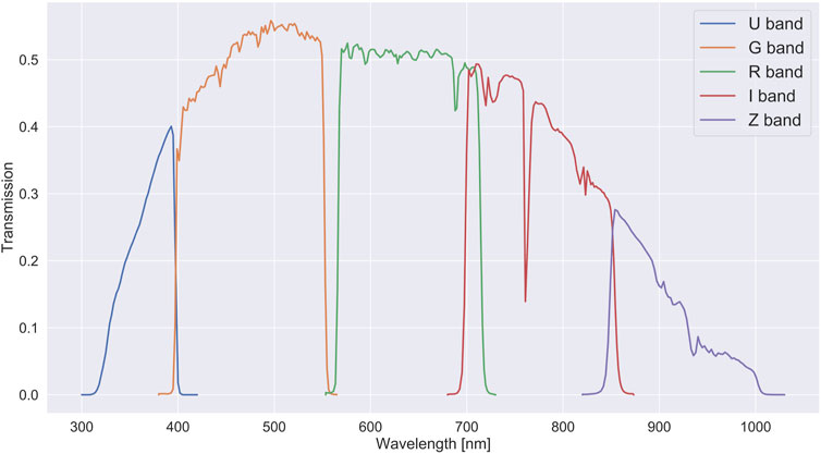
FIGURE 8. Third generation set of filters of the MegaCam instrument at the Canada–France–Hawaii Telescope that is currently being used for the Canada–France Imaging Survey. The transmission filter response includes the full telescope and 1.25 air masses of atmospheric attenuation. The full telescope includes mirrors, optics, and CCDs.

4 PSF field contributors and related degradations

So far, we have described how the PSF interacts with the images we observe and how we can model an observation. However, we have not given much information about the different PSF field contributors and the different degradations represented by F_p in Eq. 37 that can occur when modelling observations. We provide a non-exhaustive list of contributors to the PSF field, sources of known degradations, and the atmosphere’s effect on our PSF modelling problem.

4.1 Image coaddition

A fundamental contributor to the PSF is the choice of image coaddition scheme. A coadded image is a composite image created by combining multiple individual exposures of the same region of the sky in some way. This process can help increase the signal-to-noise ratio of the observation. Motivated by the analysis of the LSST data, Mandelbaum et al. (2022) have explored different coaddition schemes and studied how they affect the PSF of the resulting coadded image. In particular, Mandelbaum et al. (2022) have defined the schemes under which the coadded image accepts a well-defined PSF, i.e., the observation can be described by the convolution of an extended object and a uniquely defined coadded PSF. Bosch et al. (2017) have described the strategy for image and PSF coaddition in the HSC survey.

4.2 Dithering and super-resolution

Dithering consists of taking a series of camera exposures shifted by a fractional or a few pixel amount. There are several advantages of using a dithering strategy, which include the removal of cosmic rays and malfunctioning pixels, improving photometric accuracy, filling the gap between the detectors, and improving the sampling of the observed scene. Dithering allows estimating a sampling density of the images that is denser than the original pixel grid; in other words, to super-resolve the image. Regarding PSFs, it allows recovering Nyquist sampled PSF from undersampled observations. Bernstein (2002) studied the effect of dithering and the choice of pixel sizes in imaging strategies. Naturally, as we will see later, the dithering strategy is helpful for space-based telescopes thanks to their stability. In ground-based telescopes, the atmosphere constantly changes the PSF, making the dithering strategy less effective. However, a dithering strategy can be helpful if the telescope is equipped with adaptive optics technology, which will be described in Section 4.6. An example is the Spectro-Polarimetic High-contrast imager for Exoplanet REsearch (SPHERE) instrument (Beuzit et al., 2019) built for the European Southern Observatory’s (ESO's) Very Large Telescope (VLT) in Chile.

Lauer (1999b) discussed the limiting accuracy effect of undersampled PSFs in stellar photometry and proposed ways to correct it with dithered data (Lauer, 1999a). Fruchter and Hook (2002) presented the widely used Drizzle algorithm that consists of shifting and adding the dithered images onto a finer grid. Rowe et al. (2011) proposed a linear coaddition method coined IMCOM to obtain a super-resolved image from several undersampled images. Hirata et al. (2023) later studied the use of IMCOM on simulations (Troxel et al., 2023) from the Roman Space Telescope, while a companion paper by Yamamoto et al. (2023) explored its implications for weak-lensing analyses. Ngolè et al. (2015) proposed a super-resolution method coined SPRITE targeting the Euclid mission based on a sparse regularisation technique. More recent PSF models handle the undersampling of observations directly in their algorithms for estimating a well-sampled PSF field, as we will see later.

4.3 Optic-level contributors

These contributors affect the PSF by modifying the wave propagation in the optical system. In other words, they affect the wavefront’s amplitude and phase.

•Diffraction phenomena and aperture size: As we have seen in Section 2, the diffraction phenomena occurring in the optical system play an essential role in the formation of the PSF. The size of the optical system's aperture and the wavelength of light being studied are of particular interest. Eq. 35 shows us that under some approximations, the PSF is the Fourier transform of the aperture. Therefore, the size of the aperture and the PSF are closely related. For example, if we consider an ideal circular aperture, its diffraction pattern is the well-known Airy disk. The relationship between the width of the PSF and diameter of the aperture is given by

${\theta }_{\text{FWHM}}=1.025\frac{\lambda }{d},(40)$

where θ_FWHM is the full width at half maximum (FWHM) expressed in radians, λ is the wavelength of the light being studied, and d is the diameter of the aperture. The width of the PSF is a fundamental property of an optical system as it defines the resolution of the system. In other words, the PSF size defines the optical system’s ability to distinguish small details in the image.

•Optical aberrations: These aberrations are due to imperfections in the optical elements, e.g., a not ideally spherical mirror or not perfectly aligning optical components. The optical aberrations play a significant role in the morphology of the PSF and can be modelled using the WFE introduced in the generalised pupil function from Eq. 22. Some aberrations have a distinctive name, e.g., coma, astigmatism, and defocus, and they represent a specific Zernike polynomial (Noll, 1976).

•Surface errors or polishing effects: One would ideally like perfectly smooth surfaces in mirrors and lenses. However, imperfections arise in the optical surfaces due to imperfect surface polishing. Krist et al. (2011) showed the measurement of surface errors (SFE) in the Hubble Space Telescope (HST). Gross et al. (2006, §3.5.2) gave a more in-depth analysis of surface errors focusing on the tolerancing of SFE. Figure 9A shows the surface errors measured for the Hubble Space Telescope (HST). Krist and Burrows (1995) studied HST’s SFE before and after its iconic repair in 1993 with parametric and non-parametric (Gerchberg and Saxton, 1972) phase-retrieval algorithms.

•Obscurations: Complex optical systems have telescope designs where some elements can obscure some parts of the pupil. Obscurations are an essential contributor to PSF morphology and result from projecting a 3D structure onto the 2D focal plane. The resulting projection depends on the considered position of the focal plane. Accurate modelling of telescopes with wide-field imagers, e.g., Euclid, requires the computation of the obscuration’s position dependence arising from the 3D projection. The Euclid’s obscurations are presented in Figure 6A. Fienup et al. (1993) and Fienup (1994) studied HST’s obscuration from phase-retrieval algorithms and noticed a misalignment that caused a pupil shift.

•Stray and scattered light: Optical elements and instruments give rise to light reaching the detectors. Krist (1993) studied this problem for the HST. Storkey et al. (2004) developed methods to clean observations with scattered light from the SuperCOSMOS Sky Surveys (Hambly et al., 2001). Sandin (2014) studied the effect of scattered light on the outer parts of the PSF.

•Material outgassing and ice contamination: Material outgassing leads to molecular contamination that alters different properties of the imaging system. Water is the most common contaminant in cryogenic spacecraft, which then turns into thin ice films. A notable example is the Gaia mission which suffered from ice contamination (see Gaia Collaboration et al., 2016, §4.2.1) and required several decontamination procedures to slowly remove the ice from the optical system. Euclid Collaboration et al. (2023a) studied the ice formation and contamination for Euclid. The article also reviews the lessons learnt from other spacecraft on the topic of material outgassing. A companion paper by Euclid Collaboration et al. (2023a) is expected to be published soon that addresses the quantification of iced optics impact on Euclid’s data.

•Chromatic optical components: These components have a particular wavelength dependence, excluding the natural chromaticity due to diffraction. They are usually spectral filters and depend on the optical system design. A particular example is a dichroic filter which serves as an ideal band-pass filter. The Euclid optical system includes a dichroic filter which allows using both instruments, VIS and NISP, simultaneously as their passbands are disjoint. A dichroic filter is made of a stack of thin coatings of specific materials and thicknesses. Even if these components have a high-quality manufacturing process, they can induce significant chromatic variations in reflection that affect the PSF morphology. Baron et al. (2022) proposed a test bench to characterise Euclid’s dichroic filter and a numerical model of its chromatic dependence.

•Light polarisation: In Section 2, we studied the scalar diffraction theory, thus neglecting light polarisation. Firstly, the optical system can induce polarisation even when the incoming light is not polarised. Breckinridge et al. (2015) studied the effect of polarisation aberrations on the PSF of astronomical telescopes. The study of polarisation was carried out using Jones matrices (Jones, 1941). These matrices describe a ray’s polarisation change when going through an optical system. For more information on polarisation aberrations, see McGuire and Chipman (1990, 1991) and Yun et al. (2011). Secondly, there are some regions in space where the incoming light has been polarised by different sources, e.g., galactic foreground dust. Lin et al. (2020) studied the impact of light polarisation on weak-lensing systematics for the Roman Space Telescope (Spergel et al., 2015). The study found that the systematics introduced by light polarisation is comparable to the Roman Space Telescope’s requirements.

•Thermal variations: The thermal variations in a telescope introduce mechanical variations in its structure that affect the performance of the optical system. The origin of thermal variations is the strong temperature gradients due to the Sun’s illumination. It is sometimes referred to as the telescope’s breathing (Bély et al., 1993) for the periodical pattern consequence of its orbit. Thermal variations can introduce a small defocusing of the system that will change the PSF morphology. This phenomenon was first identified in the HST (Hasan et al., 1993). Nino et al. (2007) studied HST focus variations with temperature, and Lallo et al. (2006) studied HST temporal optical behaviour, where temperature variations play a principal role. Later works (Suchkov and Casertano, 1997; Makidon et al., 2006; Sahu et al., 2007) studied the impact of thermal variations, and consequently PSF variations, on different science applications. A Structural–Thermal–Optical Performance (STOP) test helps predict the thermal variations’ impact on the optical system. This effect is naturally more significant in space-based telescopes as the temperature gradients in space are considerably more prominent than the ones found on the ground. Space-based telescopes located at the stable L₂ Lagrange point, e.g., Euclid and James Webb Space Telescope (JWST), are less prone to thermal variations than telescopes orbiting the Earth, e.g., HST.

FIGURE 9

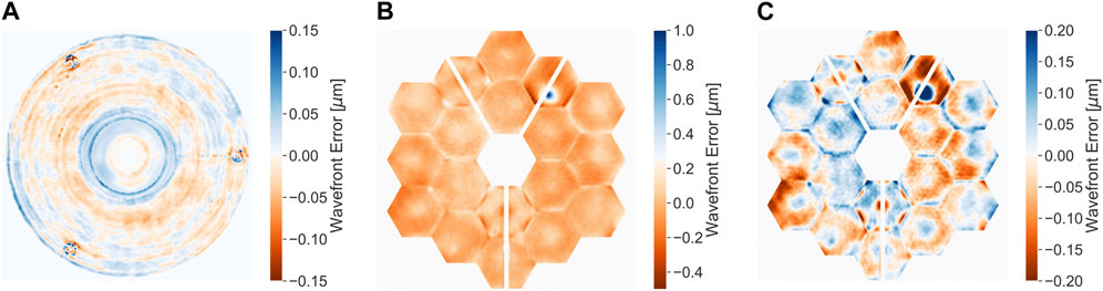
FIGURE 9. (A) Reduced range of variations to show the surface errors measured for the Hubble Space Telescope, where the scale has been reduced from ±22 nm to better show details. (B,C) Wavefront error measurements from the JWST Cycle 1 science operation on 30 July 2022 with the total and reduced range of variations, respectively.

As an example, Figures 9B,C show the measured optical contribution for the James Webb Space Telescope (JWST) PSF. Rigby et al. (2022) have presented a detailed analysis of JWST’s state, since its commissioning, which includes its PSF.

4.4 Detector-level degradations

Detector-level degradations are related to the detectors being used and, therefore, to the intensity of the PSF. They affect the observed images through the degradation operator F_p from Eq. 37, and as we will use star images, or eventually other observations, to constrain PSF models, it is necessary to consider their effects. Some of these degradations are non-convolutional and will not be well modelled by a convolutional kernel. Nevertheless, we expect that image preprocessing steps will mainly correct these effects. However, the correction will not be perfect, and some modelling errors can propagate to the observations.

•Undersampling and pixellation: The EM wave that arrives at the detectors is a continuous function. The discrete pixels in the detectors integrate the functions and measure the intensity of the wave in their respective areas. We name this process pixellation, also known as sampling. Some authors, e.g., Anderson and King (2000), Bernstein (2002), and Kannawadi et al. (2016), have defined an effective PSF as the convolution of the optical PSF, i.e., the flux distribution at the focal plane from a point source, with the pixel response of the instrument, e.g., a 2D top-hat function. High et al. (2007) performed an early study on the effects of pixellation in WL and the choice of pixel scale for a WL space-based mission. Krist et al. (2011, §3) gave some insights on the pixellation effects for the HST. Two aspects of pixellation play a crucial role in PSF modelling. Firstly, the sampling is done with the same grid, but it is indispensable to consider that the continuous function is not necessarily centred on the grid. This difference means that intra-pixel shifts between the different pixellations will be found. Figure 10 shows how two pixel representations of the same light profile change due to two different pixellations. When optimising a PSF model to reproduce some observed stars, the centroids of both images must be the same. Suppose the image centroids are the same, and the underlying model represents the observations satisfactorily. In such a case, the residual image between the two pixelated images will be close to zero. If the centroids are not the same, the residual can be far from zero even though the model is a good representation of the observation, as illustrated in the residual image in Figure 10. The second aspect is related to the Nyquist–Shannon sampling theorem. The theorem states the required number of samples that we have to use to determine perfectly a signal of a given bandwidth. In the telescopes we study, the bandwidth and number of samples are related to the aperture’s diameter and pixel size. Depending on the telescope’s design, the sampling may not verify the Nyquist–Shannon theorem. If the images are undersampled, i.e., the theorem is not verified, a super-resolution step is required in the PSF modelling, which is the case in Euclid. Using an observation strategy with dithering, as described in Section 4.2, can significantly mitigate the undesired effects of undersampling and pixellation. Kannawadi et al. (2021) studied ways of mitigating the effects of undersampling in WL shear estimations using metacalibration (Huff and Mandelbaum, 2017; Sheldon and Huff, 2017; Sheldon et al., 2020), which is a method for measuring WL shear from well-sampled galaxy images. Finner et al. (2023) studied near-IR weak-lensing (NIRWL) measurements in the CANDELS fields from HST images. The authors find that the most significant contributing systematic effect to WL measurements is caused by undersampling.

•Optical throughput and CCD quantum efficiency (QE): The optical throughput of the system is the combined effect of the different elements that compose the optical system, such as mirrors and optical elements like coatings (Venancio et al., 2016). The filter being used in the telescope forms a part of the optical throughput, as can be seen in Figure 8 for the MegaCam set of filters. Figure 8 also includes the CCD QE, which describes the sensibility of the CCD to detect photos of different wavelengths. Commonly, CCDs do not have a uniform response to the different wavelengths. Therefore, we must multiply the CCD QE with the telescope’s optical throughput to compute the total transmission.

•CCD misalignments: Ideally, we expect that all the CCDs in the detector lie in a single plane that happens to be the focal plane of the optical system. However, this is not the case in practice, as there might be small misalignments between the CCDs that introduce small defocuses that change from CCD to CCD. For a study of this effect for the Vera C. Rubin Observatory, see Jee and Tyson (2011, Figure 8).

•Guiding errors: Even if space telescopes are expected to be very stable during observations thanks to the Attitude and Orbit Control System (AOCS), there will exist a small residual motion that is called pointing jitter. The effect on the observation is the introduction of a small blur that can be modelled by a specific convolutional kernel that depends on the pointing time series. Fenech Conti (2017, §4.8.3) proposed to model the effect for Euclid with a Gaussian kernel.

•Charge transfer inefficiency: CCD detectors are in charge of converting incoming photons to electrons and collecting them in a potential well in the pixel during an exposure. The charge on each pixel is read when the exposure is complete. The collected electrons are transferred through a chain of pixels to the edge of the CCD, amplified, and then read. High-energy radiation above the Earth’s atmosphere gradually damages the CCD detector (Prod’homme et al., 2014b; Prod’homme et al., 2014a). The silicon damage in the detectors creates traps for the electrons that are delayed during the reading procedure. This effect is known as charge transfer inefficiency (CTI), producing a trailing of bright objects and blurring the image. This effect is noticeably significant for space telescopes, given the harsh environment. CTI effects are expected to be corrected in the VIS image preprocessing. Rhodes et al. (2010) carried out a study on the impact of CTI on WL studies. Massey et al. (2009) developed a model to correct CTI for the HST and later improved it in Massey et al. (2014).

•Brighter-fatter effect: The assumption that each pixel photon count is independent of its neighbours does not hold in practice. There is a photoelectron redistribution in the pixels as a function of the number of photoelectrons in each pixel. The brighter-fatter effect (BFE) is due to the accumulation of charge in the pixels’ potential wells and the build-up of a transverse electric field. The effect is stronger for bright sources. Antilogus et al. (2014) studied the effect and observed that the images from the CCDs do not scale linearly with flux, so bright star sizes appeared larger than fainter stars. Guyonnet et al. (2015) and Coulton et al. (2018) proposed methods to model and correct this effect. The preprocessing of VIS images is supposed to correct for the BFE, but there might be some residuals.

•Wavelength-dependent sub-pixel response: There exists a charge diffusion between neighbouring pixels in the CCD. Niemi et al. (2015) studied this effect for Euclid’s VIS CCD and modelled the response of the CCD. They proposed to model the effect as a Gaussian convolutional kernel where the standard deviations of the 2D kernel are wavelength dependent: σ_x(λ) and σ_y(λ). They measured the proposed model with a reference VIS CCD. Krist (2003) studied the charge diffusion in the HST and proposed spatially varying blur kernels to model the effect.

•Noise: There are several noise sources in the measurements. Thermal noise (Nyquist, 1928) refers to the signal measured in the detector due to the random thermal motion of electrons which is usually modelled as Gaussian. Readout noise (Basden et al., 2004) refers to the uncertainty in the photoelectron count due to imperfect electronics in the CCD. Dark-current shot noise (Baer, 2006) refers to the random generation of electrons in the CCD, and even though it is related to the temperature, it is not Gaussian. There are also unresolved and undetected background sources that contribute to the observation noise. These are the statistics of the predominant noise that depends on the imaging setting of the instrument and its properties.

•Tree rings and edge distortions: There exist electric fields in the detector that are transverse to the surface of the CCD. The origin of these fields includes doping gradients or physical stresses on the silicon lattice. This electric field displaces charge, modifying the effective pixel area. Consequently, it changes the expected astrometric and photometric measurements. This electric field also generates concentric rings, tree rings, and bright stripes near the boundaries of the CCD, edge distortions. Given the close relationship between this effect and the detector, its importance depends strongly on the instrument being used. This effect is unnoticeable in the MegaCam used in the Canada–France Imaging Survey (CFIS) as it depends on the CCD design. However, it is a major concern in the Dark Energy Camera that is used in the Dark Energy Survey (DES), as was shown by Plazas et al. (2014). Jarvis et al. (2020, Figure 9) illustrated the consequence of tree rings in PSF modelling.

•Other effects: These include detector nonlinearity (Stubbs, 2014; Plazas et al., 2016), sensor interpixel correlation (Lindstrand, 2019), interpixel capacitance (McCullough, 2008; Kannawadi et al., 2016; Donlon et al., 2018), charge-induced pixel shifts (Gruen et al., 2015), persistence (Smith et al., 2008a; Smith et al., 2008b), reciprocity failure (flux-dependent nonlinearity) (Bohlin et al., 2005; Biesiadzinski et al., 2011), and detector analogue-to-digital nonlinearity.

FIGURE 10

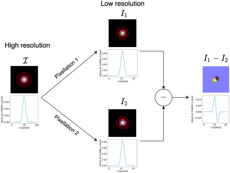
FIGURE 10. Example of two different pixellations on the same high-resolution image representing an Airy PSF. The difference between the two pixellations is an intra-pixel shift of (Δx, Δy) = (0.35, 0.15) between them. Figure reproduced from Liaudat (2022).

4.5 Atmosphere

The atmosphere plays a central role in ground-based telescopes’ PSFs. For an in-depth study of the subject, see Roddier (1981). How the atmosphere affects our images will strongly depend on the exposure time used to image an object. The PSF induced by the atmosphere for a very short exposure will look like a speckle, while a long exposure will produce a PSF that resembles a 2D Gaussian, or more precisely, a Moffat profile (Moffat, 1969). Figure 12 shows examples of atmospheric PSFs with different exposure times. The atmosphere’s effect on the PSF for a long exposure can be approximated by the effect of a spatially varying low-pass filter, thereby broadening the PSF and limiting the telescope’s resolution. Astronomers usually use the term seeing to refer to the atmospheric conditions of the telescope, and it is measured as the FWHM of the PSF. The loss of resolution due to the atmosphere is one of the main motivations for building space telescopes like Euclid and Roman, where the PSF is close to the diffraction limit and very stable.

The atmosphere is a heterogeneous medium whose composition changes with the three spatial dimensions and time. The inhomogeneity of the atmosphere affects the propagation of light waves that arrive at the telescope. Instead of supposing that the incoming light waves are plane, as emitted by the faraway source under study, these waves already have some phase lags or leads with respect to an ideal plane wave. The atmosphere introduces a WFE contribution to the optical system. These effects can be resumed as an effective phase-shifting plate, Φ_eff(x, y, t). However, calculating this effective plate is cumbersome as it involves having a model of the atmosphere and integrating the altitude, z, so that we have the spatial distribution, (x, y), of the effective WFEs. The model of the atmosphere is represented by the continuous $C_n^2(z)$ (Roddier, 1981) profile, which represents the variations of the refractive index due to atmospheric turbulence as a function of height. However, the $C_n^2(z)$ is challenging to model and measure, and even if it is possible, it is computationally expensive to exploit.

We can discretise the integral over the altitude into M thin phase screens of variable strengths at different altitudes to simulate the effect of the atmosphere. Each phase screen will have specific properties and move at different speeds in different directions. These assumptions are known as the frozen flow hypothesis. Each phase screen will be characterised by its power spectrum that can be modelled by a von Kármán model of turbulence (Kármán, 1930). The power spectrum of the atmosphere’s WFE contribution is given by

$\mathrm{\Psi }\left(\nu \right)=0.023r_0^{-5/3}{\left({\nu }^2+\frac{1}{L_0^2}\right)}^{-11/6},(41)$

where ν is the spatial frequency, r₀ is the Fried parameter, and L₀ is the outer scale. Both parameters, r₀ and L₀, are generally expressed in metres. The Fried parameter relates to the turbulence amplitude, and the outer scale relates to the correlation length. For an example of atmospherical phase screens, see Figure 11. For lengths longer than L₀, the power of the turbulence asymptotically flattens. If we take the limit of L₀ to infinite, we converge to the Kolmogorov model of turbulence (Kolmogorov, 1991). For more information on electromagnetic wave propagation in turbulence, see Sasiela (1994).

FIGURE 11

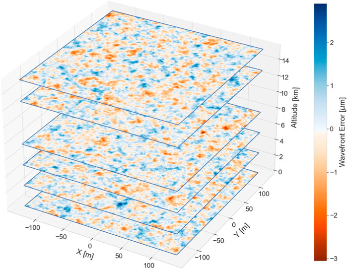
FIGURE 11. Illustration of six von Kármán phase screen layers at different altitudes simulated for LSST. The simulations were produced with the GalSim package (Rowe et al., 2015) using the parameters from Jee and Tyson (2011).

Once the phase screens, Φ_m(x, y|u_i, v_i), have been simulated following Eq. 41, the temporal variation of the screen has to be taken into account. The phase screens contribute to the WFEs of the PSF, which is why it depends on the pupil plane variables (x, y). The temporal variation is usually modelled with the wind’s properties at the phase screen’s reference altitude. We describe the wind with two components, v_u and v_v, where we have assumed that v_z = 0. We then obtain the effective phase screen by a weighted average of the phase screens at the different altitudes as

${\mathrm{\Phi }}_{\text{eff}}\left(x,y;t|u_i,v_i\right)=\sum _{m=1}^M{c}_m{\mathrm{\Phi }}_m\left(x,y;t|u_i,v_i\right),(42)$

where {c_m} are relative weights corresponding to the different phase screen. The difficulty of modelling the atmosphere is that the time scales are comparable with the exposure time. Therefore, the PSF that we estimate for a given time snapshot will change with respect to another PSF at another snapshot within the same camera exposure. This change means that we have to integrate the instantaneous PSF over time to model the PSF physically, which corresponds to

$I_{\text{img}}\left(\bar{u},\bar{v}|u_i,v_i\right)={\int }_{t_0}^{t_0+T_{\text{exp}}}{I}_{\text{img}}\left(\bar{u},\bar{v};t|u_i,v_i\right)dt,(43)$

where $I_{\text{img}}(\bar{u},\bar{v},t|u_i,v_i)$ is the instantaneous image of the object affected by the PSF $\mathcal{H}(u,v;\lambda ;t|u_i,v_i)$, t₀ is a random initial time, and T_exp is the exposure time.

Finally, we have to choose the time step size to discretise the integral from Eq. 43. Each instantaneous PSF will look like a speckle. Once we add them up in the integral, the PSF starts to become rounder and smoother. Figure 12 shows examples of atmospheric PSFs using different exposure times that were simulated using six-phase screens using the parameters from Jee and Tyson (2011) that correspond to an LSST-like scenario. It is interesting to see how the short-exposure PSF looks like a speckle, and then the profile becomes more and more smooth as the exposure time increases. As a reference, the exposure time used for the r-band observations in CFIS is 200 s⁴. de Vries et al. (2007) studied the PSF ellipticity change due to atmospheric turbulences as a function of the exposure time. They observed that the ellipticity of the PSF decreases its amplitude as the exposure time increases.

FIGURE 12

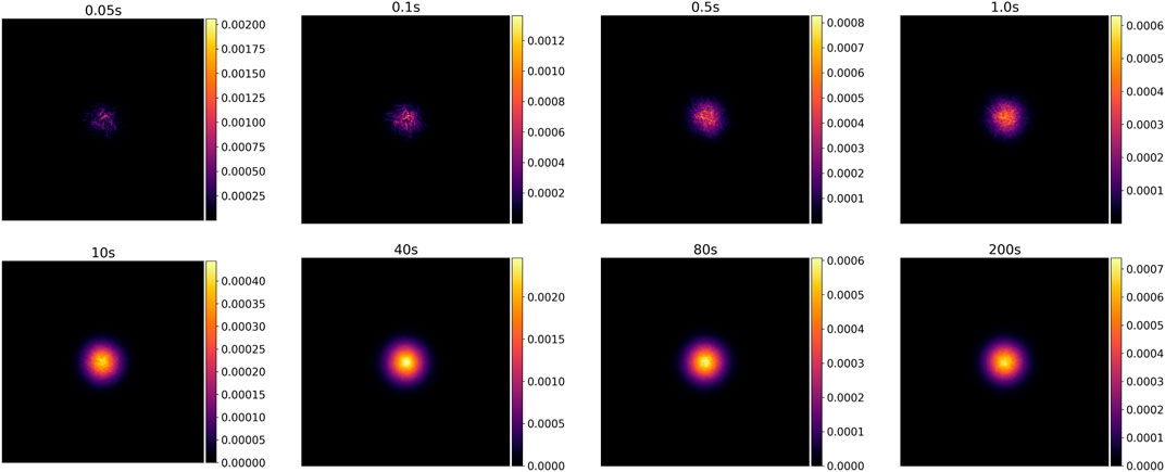
FIGURE 12. Example of atmospheric PSFs with different exposure times. The simulation was done using the atmospherical parameters from Jee and Tyson (2011) for an LSST-like scenario.

Another effect that should be considered is atmospheric differential chromatic refraction. This effect represents the refraction due to the change of medium from vacuum to the Earth’s atmosphere. The effect varies as a function of the zenith angle and wavelength. Meyers and Burchat (2015b) performed a study on the impact of the atmospheric chromatic effect on weak lensing for surveys like LSST and DES.

Heymans et al. (2012) performed a study on the impact of atmospheric distortions on weak-lensing measurement with real data from CFHT. They characterised the ellipticity contribution of the atmosphere to the PSF for different exposure times. To achieve this, they computed the two-point correlation function of the residual PSF ellipticity between the observations and a PSFEx-like PSF model (described in detail in Section 5). Salmon et al. (2009) studied the image quality and the observing environment at the CFHT (Xin et al., 2018) and carried out a study of the PSF and the variation of its width with time and wavelength for the Sloan Digital Sky Survey (SDSS) (Gunn et al., 1998; York et al., 2000). Jee and Tyson (2011) carried out a simulation study to evaluate the impact of atmospheric turbulence on weak-lensing measurement in LSST. Jee and Tyson (2011) used the atmospherical parameters from (Ellerbroek, 2002) that were measured in the LSST site in Cerro Pachón, Chile. There is an ongoing project at LSST DESC⁵ to leverage atmospheric and weather information at or near the observation site to produce realistically correlated wind and turbulence parameters for atmospheric PSF simulations.

Another way to simulate the atmosphere and the PSF is to use a photon Monte Carlo approach. This line of work was carried out in Peterson et al. (2015, 2019, 2020) with a simulator available coined⁶ that is capable of simulating several telescopes including the Vera C. Rubin observatory and JWST. The method consists of sampling photons from astronomical sources and simulating their interactions with their models of the atmosphere, the optics and the detectors. PhoSim is characterised by being a remarkably fast simulator regarding the level of simulation complexity handled. This simulator has proved helpful in several studies (Walter, 2015; Xin et al., 2015; Beamer et al., 2015; Carlsten et al., 2018; Xin et al., 2018; Burke et al., 2019; Sánchez et al., 2020; Nie et al., 2021b; Euclid Collaboration, 2023b; Euclid Collaboration, 2023c; Merz et al., 2023). PhoSim is a powerful simulation tool that can help to study the PSF of systems by following a forward model approach where simulations are compared with observations (Chang et al., 2012; Chang and Peterson, 2017). The PhoSim parameters can then be fitted or modified to match the simulation output with the observed images. Another known simulation software⁷, Rowe et al. (2015), incorporates options to simulate atmospheric PSFs from phase-screen exploiting the photon Monte Carlo approach from Peterson et al. (2015).

To conclude, we have seen that it is possible to develop a physical model of the atmosphere based on the optical understanding that we have from Section 2 and the studies of atmospheric turbulence of Kármán and Kolmogorov. However, this approach has two inconveniences. Firstly, the approach requires physical measurements of the atmosphere at the telescope’s site, which is not always available. Secondly, it is computationally expensive, as there is an altitude and a temporal integration to handle varying atmospherical properties and reach the exposure time, respectively. In practice, it is required to use long exposure times to obtain deeper observations, i.e., observing fainter objects that are important for weak-lensing studies. This fact simplifies the PSF modelling task as the long temporal integration smooths the PSF profile and PSF spatial variations over the FOV. Therefore, a data-driven approach to modelling the PSF can offer a feasible and effective solution in this scenario.

4.6 Adaptive optics

An alternative approach to work with ground-based observations affected by the atmosphere is to use adaptive optics (AO) systems (Beckers, 1993). This technology significantly improves the observation resolution in ground-based telescopes that is severely limited due to the atmosphere, as we have seen in Section 4.5. An AO system tries to counteract the effect of the atmosphere on the incoming wavefront by changing the shape of a deformable mirror. The key components of the AO system are wavefront sensors (WFS), wavefront reconstruction techniques, and deformable mirrors, which operate together inside a control loop. The WFS provides information about the incoming wavefront and usually incorporates a phase-sensitive device. The wavefront reconstruction has to compute a correction vector for the deformable mirrors by estimating the incoming wavefront from the WFS information. The control loop works in real-time sensing and modifies the deformable mirrors so that the wavefront received by the underlying instrument is free from optical path differences introduced by the atmosphere. Davies and Kasper (2012) have provided a detailed review of the AO systems for astronomy. The LSST that carries out weak-lensing studies contains an AO system (Angeli et al., 2014; Neill et al., 2014; Thomas et al., 2016). Exoplanet imaging studies have greatly benefited from AO systems and impose strict requirements for these systems. Some examples are the SPHERE instrument in the VLT (Beuzi et al., 2019) and the Gemini Planet Imager (Graham et al., 2007; Macintosh et al., 2014; Macintosh et al., 2018) in the Gemini South Telescope.

5 Current PSF models

Let us now discuss some of the most known PSF models, which can be divided into two main families, parametric and non-parametric, also known as data-driven.

5.1 Parametric PSF models

This family of PSF models is characterised by trying to build a physical optical system model that aims to be as close as possible to the telescope. Once the physical model is defined, a few parameters are estimated using star observations. Such an estimation, also called calibration, is required as some events, like launch vibrations, ice contaminations, and thermal variations, introduce significant variations in the model. These events prevent a complete on-ground characterisation from being a successful model. Parametric models are capable of handling chromatic variations of the PSF as well as complex detector effects. Nevertheless, parametric models have only been developed for space missions and are custom-made for a specific telescope. The parametric model is compelling if the proposed PSF model matches the underlying PSF field. However, if there are mismatches between both models, significant errors can arise due to the rigidity of the parametric models. The difficulty of building a physical model for the atmosphere, already discussed in Section 4.5, makes them impractical for ground-based telescopes.

The parametric model Tiny Tim⁸ (Krist, 1993; Krist, 1995; Krist et al., 2011) has been used to model the PSF of the different instruments on board the HST. The Advanced Camera for Surveys (ACS) in the HST was used to image the Cosmic Evolution Survey (COSMOS), which covers a 2-deg² field that was used to create a widely used space-based weak-lensing catalogue. The first WL shape catalogue used the Tiny Tim model (Leauthaud et al., 2007). Rhodes et al. (2007) studied the stability of the HST’s PSF, noticing a temporal change of focus in the images. In addition to the parametric Tiny Tim model, Anderson and King (2000) developed the concept of effective PSF, which is the continuous PSF arriving at the detectors, i.e., Equation 35, convolved with the pixel-response function of the detector. They proposed an algorithm to model the effective PSF iteratively from observed stars and continued the work on the effective PSF, adding some improvements and detailed a model for the HST instruments ACS and Wide Field Camera (WFC). Hoffmann and Anderson (2017) then carried out a comparison between Tiny Tim and the effective PSF approach for ACS/WFC. The study showed that the effective PSF approach consistently outperforms the Tiny Tim PSFs, exposing the limitations of parametric modelling. Anderson (2016) describes the adoption of the effective PSF approach applied to Wide Field Camera 3 (WFC3/IR) observations, which are undersampled. The software Photutils⁹ (Bradley et al., 2022) provides an implementation of the effective PSF approach from Anderson and King (2000) with enhancements from Anderson (2016). Schrabback, T. et al. (2010) used a data-driven PSF model based on PCA when studying the COSMOS field.

The early severe aberrations of HST’s optical system were an important driver of phase-retrieval algorithms. Several efforts to characterise HST were published in an Applied Optics special issue (Breckinridge and Wood, 1993). Solving the phase-retrieval problem provides a reliable approach to characterise the optical system accurately. Fienup (1993) studied new phase-retrieval algorithms and Fienup et al. (1993) presented several results characterising HST’s PSF.

Regarding recently launched space telescopes, Euclid’s VIS parametric model constitutes the primary approach for Euclid’s PSF modelling. The model will soon be published and used to work with observations from Euclid. JWST has a Python-based simulating toolkit, WebbPSF¹⁰ (Perrin et al., 2012, 2014). Recent works have developed and compared data-driven PSF models for JWST’s NIRCam (Nardiello et al., 2022; Zhuang and Shen, 2023).

5.2 Data-driven (or non-parametric) PSF models

The data-driven PSF models, also known as non-parametric, only rely on the observed stars to build the model in pixel space. They are blind to most of the physics of the inverse problem. These models assume regularity in the spatial variation of the PSF field across the FOV and usually differ in how they exploit this regularity. Data-driven models can easily adapt to the current state of the optical system. However, they have difficulties modelling complex PSF shapes occurring in diffraction-limited settings. One limitation shared by all the data-driven models is their sensitivity to the available number of stars to constrain their estimation. A low star number implies that there might be not enough stars to sample the spatial variation of the PSF. When the number of stars in an FOV falls below some threshold, the model built is usually considered unusable for WL purposes. This family of models has been widely used for modelling ground-based telescope PSFs. Nevertheless, they are not yet capable of successfully modelling the chromatic variations in addition to the spatial variations and super-resolution.

We proceed by describing several PSF models in chronological order. The first models, described in more detail, were used to process real data from different surveys, except for Resolved Component Analysis (Ngolè et al., 2016). The latter models are worth mentioning but have yet to be used to produce a WL shape catalogue with all the validation and testing it implies.

5.2.1 Shape interpolation

The first approach for PSF modelling consisted of estimating some parameters of the PSF at the positions of interest. It was done for early studies in WL and is closely related to the widely employed galaxy shape measurement method KSB (Kaiser et al., 1995). This precursor method only required the PSF’s ellipticity and size at the positions of the galaxies. Therefore, a full-pixel image of the PSF was unnecessary. Then, the KSB method can correct the galaxy shape measurement for the effects of the PSF. The method to interpolate the shape parameters to other positions is usually a polynomial interpolation. For example, this was the case for the early WL study of Canada-France-Hawaii Telescope Legacy Survey (CFHTLS) (Fu, L. et al., 2008). Gentile et al. (2013) reviewed the different interpolation methods and studied their performance for WL studies. Viola et al. (2011) performed a study showcasing different biases present in the KSB (Kaiser et al., 1995) method. These biases are a consequence of problematic KSB assumptions: 1) KSB gives a shear estimate per individual image and then takes an average, while WL shear should be estimated from averaged galaxy images; 2) KSB works under the assumption that galaxy ellipticities are small, but in the context of weak lensing, what is considered ‘small’ pertains to the alteration in ellipticity caused by the shear; and 3) KSB gives an approximate PSF correction that only holds in the limit of circular sources and does not invert the convolution with the PSF. Recent WL studies no longer use this approach. The WL studies have evolved to more sophisticated galaxy shape measurement techniques that require a full pixel image of the PSF at the position of galaxies.

5.2.2 Principal component analysis

The principal component analysis is a widely known method for multivariate data analysis and dimensionality reduction. Let us start with a set of star observations in ${\mathbb{R}}^{p^2}$ that we concatenate in a matrix $\bar{\mathbf{I}}=[{\bar{I}}_1,\dots ,{\bar{I}}_n]$. We have flattened the 2D images into an array to simplify expressions. One would like to represent the observations with r components ${\{X_i\}}_{i=1}^r$ in ${\mathbb{R}}^{p^2}$, where r ≥ n, assuming that p² > n. The PCA method gives r orthonormal components in ${\mathbb{R}}^{p^2}$ which define directions in the ${\mathbb{R}}^{p^2}$ space where the variance of the data set $\bar{\mathbf{I}}$ is maximized.

If n components are used to represent the observations, then the learned components in the PCA procedure represent a basis of the subspace spanned by the observations or the columns of $\bar{\mathbf{I}}$. The method can be interpreted as a linear transformation to a new representation with orthogonal components. As it is usual to observe regularity in the spatial variations of the PSF, most of the data set variability can be described with a few components. Then, one can only use the first r principal components and achieve a dimensionality reduction of the observations. The dimensionality reduction technique allows denoising the model as the observational noise cannot be represented with r components and only the PSF trends are well described.

The PCA method was used to model the PSF for the SDSS (Lupton et al., 2001), although it was referenced as the Karhunen–Loève transform. Jarvis and Jain (2004) then proposed its use in a WL context. Jee et al. (2007) used the PCA to model the spatial and temporal variations of the HST PSF. Jee and Tyson (2011) also used the PCA to model the PSF in LSST simulations. HST’s COSMOS catalogue (Schrabback, T. et al., 2010) used the PCA to model the PSF. The PCA showcased the utility and robustness of data-driven methods and the importance of using a pixel representation of the PSF and is the precursor of several of the following models.

5.2.3 PSFEx

PSFEx¹¹ (Bertin, 2011) has been widely used in astronomy for weak-lensing surveys, e.g., DES year 1 (Zuntz et al., 2018), HSC (Mandelbaum et al., 2017), and CFIS (Guinot et al., 2022). It was designed to work together with the SExtractor (Bertin and Arnouts, 1996) software which builds catalogues from astronomical images and measures several properties of the observed stars. The PSFEx models the variability of the PSF in the FOV as a function of these measured properties. It builds independent models for each CCD in the focal plane and works with polychromatic observations. It cannot model the chromatic variations of the PSF field. The model is based on a matrix factorisation scheme, where one matrix represents the PSF features and the other matrix represents the feature weights. Each observed PSF is represented as a linear combination of PSF features. The feature weights are defined as a polynomial law of the selected measured properties. This choice allows having an easy interpolation framework for target positions. In practice, the properties that are generally used are both components of the PSF’s FOV position. The PSF features are shared by all the observed PSFs and are learnt in an optimisation problem. The PSF reconstruction at a FOV position (u_i, v_i) can be written as

${\bar{I}}_{\text{star}}^{\text{PSFEx}}\left(\bar{u},\bar{v}|u_i,v_i\right)=F^{\text{PSFEx}}\underset{{\bar{H}}^{\text{PSFEx}}\left(\bar{u},\bar{v}|u_i,v_i\right)}{\underbrace{\left\{\sum _{\begin{array}{c}p,q\ge 0\\ p+q\le d\end{array}}{u}_i^p{v}_i^q{S}_{p,q}\left(\bar{u},\bar{v}\right)+S_0\left(\bar{u},\bar{v}\right)\right\}}},(44)$

where ${\bar{I}}_{\text{star},(\cdot |u_i,v_i)}^{\text{PSFEx}}\in {\mathbb{R}}^{p\times p}$ is the PSFEx reconstruction of the observed star ${\bar{I}}_{(\cdot |u_i,v_i)}$, $S_{p,q}\in {\mathbb{R}}^{P\times P}$ represents the learned PSF features or eigenPSFs, $S_0\in {\mathbb{R}}^{P\times P}$ represents the first guess of the PSF, the polynomial law is defined to be of degree d, and F^PSFEx represents the degradations required to match the model with the observations. The model’s PSF reconstruction is represented by ${\bar{H}}^{\text{PSFEx}}$. The first guess can be computed as a function of the median of all the observations. The dimensions p and P are the same if no downsampling operation is included in F^PSFEx.

The PSF features are learnt in an optimisation problem that aims to minimise the reconstruction error between the PSFEx model and observations, which are given by

$\underset{\begin{array}{c}{S}_{p,q}\\ \forall p,q\ge 0,p+q\le d\end{array}}{\min }\left\{\sum _{i=1}^{n_{\text{obs}}}{‖\frac{{\bar{I}}_{\left(\cdot |u_i,v_i\right)}-{\bar{I}}_{\text{star},\left(\cdot |u_i,v_i\right)}^{\text{PSFEx}}}{{\widehat{\sigma }}_i}‖}_F^2+\sum _{\begin{array}{c}p,q\ge 0\\ p+q\le d\end{array}}{‖T_{p,q}{S}_{p,q}‖}_F^2\right\},(45)$

where ${\widehat{\sigma }}_i^2$ represents the estimated per-pixel variances, $\bar{I}$ represents the noisy observations, and ‖ ⋅‖_F the Frobenius norm of a matrix. The second term in Eq. 45 corresponds to a Tikhonov regularisation, where T_p,q represents some regularisation weights to favour smoother PSF models. The PSF recovery at target positions is straightforward. One has to introduce new positions in Eq. 44 after learning the PSF features S_p,q. The recovery at a new FOV position (u_j, v_j) is simply given by

${\bar{H}}^{\text{PSFEx}}\left(\bar{u},\bar{v}|u_j,v_j\right)=\sum _{\begin{array}{c}p,q\ge 0\\ p+q\le d\end{array}}{u}_j^p{v}_j^q{S}_{p,q}\left(\bar{u},\bar{v}\right)+S_0\left(\bar{u},\bar{v}\right),(46)$

where ${\bar{H}}^{\text{PSFEx}}$ is the model’s PSF reconstruction, and S₀ and S_p,q are learnt during the training procedure.

5.2.4 Resolved component analysis

The resolved component analysis (RCA)¹² (Ngolè et al., 2016) is a state-of-the-art data-driven method designed for the space-based Euclid mission (Schmitz et al., 2020). The model builds an independent model for each CCD, can handle super-resolution, and, like the PSFEx, is based on a matrix factorisation scheme. However, there are three fundamental changes with respect to the PSFEx. The first difference is that, in RCA, the feature weights are defined as a further matrix factorisation and are also learnt from the data. The feature weights are constrained to be part of a dictionary¹³ built with different spatial variations based on the harmonics of a fully connected undirected weighted graph. The graph is built using the star positions as the nodes and a function of the inverse distance between the stars to define the edge weights. The rationale of the graph-harmonics dictionary is to capture localised spatial variations of the PSF that occur in space-based missions exploiting the irregular structure of the star positions. The RCA reconstruction of an observed star is then

$\begin{array}{ll}\hfill {\bar{I}}_{\text{star}}^{\text{RCA}}\left(\bar{u},\bar{v}|u_i,v_i\right)& =F^{\text{RCA}}\left\{{\bar{H}}^{\text{RCA}}\left(\bar{u},\bar{v}|u_i,v_i\right)\right\},\text{\hspace{0.17em}where}\hfill \\ \hfill {\bar{H}}^{\text{RCA}}\left(\bar{u},\bar{v}|u_i,v_i\right)& =\sum _{r=1}^{N_{\text{comp}}}{S}_r\left(\bar{u},\bar{v}\right)A\left[r,i\right]\hfill \\ \hfill & =\sum _{r=1}^{N_{\text{comp}}}{S}_r\left(\bar{u},\bar{v}\right)\left(\alpha V^{\top }\right)\left[r,i\right],\hfill \end{array}(47)$

where ${\bar{I}}_{\text{star},(\cdot |u_i,v_i)}^{\text{RCA}}\in {\mathbb{R}}^{p\times p}$ , F ^RCA corresponds to the degradation model of the RCA, which includes downsampling, intra-pixel shifts, among others, $S_r\in {\mathbb{R}}^{Dp\times Dp}$ corresponds to the data-driven feature, i.e., eigenPSF, r from a total of N _comp features, D is the upsampling factor in case a super-resolution step is required, and A [r, i] is the rth feature weight of the ith star. The feature weight matrix A is decomposed into a sparse matrix α and a dictionary matrix V ^⊤ of graph-based spatial variations; for more information, see Ngolè et al. (2016).

To regularise the inverse problem, the RCA enforces a low-rank solution by fixing N _comp, a positivity constraint on the modelled PSF, a denoising strategy based on a sparsity constraint in the starlet (Starck et al., 2015) domain, which is a wavelet representation basis, and a constraint to learn the useful spatial variations from the graph-harmonics-based dictionary. The optimisation problem that the RCA method targets is

$\begin{array}{ll}\hfill & \underset{S_k,{\alpha }_k}{\min }\left\{\frac{1}{2}\sum _{i=1}^{n_{\text{obs}}}\right.{‖{\bar{I}}_{\left(\cdot |u_i,v_i\right)}-F^{\text{RCA}}\left\{{\bar{H}}_{\left(\cdot |u_i,v_i\right)}^{\text{RCA}}\right\}‖}_F^2\hfill \\ \hfill & +\sum _{r=1}^{N_{\text{comp}}}\Vert w_r\odot \mathrm{\Phi }{S}_r{\Vert }_1+\left.{\iota }_{+}\left({\bar{H}}_{\left(\cdot |u_i,v_i\right)}^{\text{RCA}}\right)+{\iota }_{\mathrm{\Omega }}\left(\alpha \right)\right\}\text{s.t.\hspace{0.17em}}\hfill \\ \hfill & {\bar{H}}_i^{\text{RCA}}=\sum _{r=1}^{N_{\text{comp}}}{S}_r\left(\alpha V^{\top }\right)\left[r,i\right],\hfill \end{array}(48)$

where w _r is the weight, Φ represents a transformation allowing the eigenPSFs to have a sparse representation, e.g., a wavelet transformation, ⊙ denotes the Hadamard product, ι ₊ is the indicator function of the positive orthant, and ι _Ω is the indicator function over a set Ω, which is defined as a set of sparse vectors and is used to enforce sparsity on α.

The second difference with respect to PSFEx corresponds to the regularisations used in the objective function from Eq. 48, which ends up being non-convex due to matrix factorisation and non-smooth due to the ‖ ⋅‖₁ constraint. The optimisation is solved through a block coordinate descent, as it is a multi-convex problem, and proximal optimisation algorithms that tackle the non-smooth subproblems (Beck and Teboulle, 2009; Condat, 2013).

The third difference is handling the PSF recovery at a new position (u _j , v _j ). The recovery is carried out by a radial basis function (RBF) interpolation of the learned columns of the A matrix, issuing a vector, ${\widehat{\mathbf{a}}}_j\in {\mathbb{R}}^{N_{\text{comp}}}$ ; for more details, see Schmitz et al. (2020). This way, the spatial constraints encoded in the A matrix are preserved when estimating the PSF at galaxy positions. The interpolated feature weights ${\widehat{\mathbf{a}}}_j$ can be introduced in the Eq. 47 formulation to generate the PSF at the new j position.

The RCA model has yet to be used to generate a WL shape catalogue from real observations. Liaudat et al. (2021a) showed that the RCA is not robust enough to handle real ground-based observations from CFIS as some CCDs exhibited significant errors in the PSF shape.

5.2.5 Multi-CCD PSF model

The multi-CCD (MCCD) ¹⁴ (Liaudat et al., 2021a) model is a state-of-the-art data-driven method originally designed for the ground-based CFIS from the CFHT. The MCCD can model the full focal plane at once by incorporating the CCD mosaic geometry into the PSF model. The MCCD model rationale is explained by the limitations of other PSF models that build independent PSF models for every CCD, e.g., RCA and PSFEx: 1) fundamentally limited in the possible model complexity due to the lack of constraining power of a reduced number of star observations, and 2) the difficulty of modelling PSF spatial variations spanning the entire focal plane, i.e., several CCDs, from independently modelled CCDs. The MCCD overcomes these issues by building a PSF model containing two types of variations: global and CCD-specific. Both variations are modelled by a matrix factorisation approach, building over the success of PSFEx and RCA. The global features are shared between all CCDs, and the local CCD-specific features aim to provide corrections for the global features. The feature weights are defined as a combination of the polynomial variations from PSFEx and the graph-based variations from RCA. The model’s optimisation is more challenging than the previous models and is based on a novel optimisation procedure based on iterative schemes involving proximal algorithms (Parikh and Boyd, 2014).

The MCCD model has proven robust enough to handle real observations from CFIS (Liaudat et al., 2021a), giving state-of-the-art results. It has been incorporated into the recent ShapePipe shape measurement pipeline (Farrens, S. et al., 2022) originally designed to process the CFIS survey and generate a WL shape catalogue. The first version of the shape catalogue (Guinot et al., 2022), spanning 1,700 deg², from ShapePipe used PSFEx. However, the next version, spanning $\sim 3500{\text{deg}}^2$ , uses the MCCD PSF model and will be released soon.

5.2.6 lensfit

The lensfit (Miller et al., 2007; Kitching et al., 2008; Miller et al., 2013) refers to a Bayesian galaxy shape measurement method for WL surveys. It also includes a data-driven PSF model that will also be referenced as lensfit and is sparsely described throughout the different publications involving the shape measurement lensfit (Miller et al., 2013; Kuijken et al., 2015; Giblin et al., 2021). This method has been used with real data to produce the WL shape catalogues of CFHTLenS (Erben et al., 2013; Miller et al., 2013), KiDS+VIKING-450 (Wright et al., 2019), KiDS-450 (Hildebrandt et al., 2016; Fenech Conti et al., 2017), KiDS-1000 (Giblin et al., 2021), and VOICE (Fu et al., 2018). However, the code is not publicly available.

This PSF model differs from the previous ones. The PSFEx and RCA learn some features or eigenPSFs that all the PSFs share. The lensfit model is fitted on a pixel-by-pixel basis. Each pixel is represented as a polynomial model of degree d of the FOV positions. The lensfit model can use all the observations in one exposure, i.e., it uses several CCDs at once. The model uses the low-order polynomials, up to degree n _c < d, to be fitted independently for each CCD, and the rest of the monomials are fitted using the observations from all the CCDs. This multi-CCD modelling is a significant change with respect to previous methods that built independent models for each CCD. The total number of coefficients per pixel is given by

$N_{\text{coeff}}=\frac{1}{2}\left(\left(d+1\right)\left(d+2\right)+\left(N_{\text{CCD}}-1\right)\left(n_{\text{c}}+1\right)\left(n_{\text{c}}+2\right)\right),(49)$

where N _CCD is the total number of CCDs in the camera, d represents the degree of the polynomial varying in the full FOV, and n _c is the polynomial that is CCD-dependent. We can write the description of the pixel $(\bar{u},\bar{v})$ of the PSF model for a FOV position (u _j , v _j ) in CCD k as follows:

${\bar{H}}^{\text{lensfit}}\left(\bar{u},\bar{v}|u_j,v_j\right)=\sum _{\begin{array}{c}p,q\ge 0\\ p+q\le d\end{array}}{u}_j^p{v}_j^q{a}_{\left(p,q\right),\left(\bar{u},\bar{v}\right)}^k+\sum _{\begin{array}{c}p+q>n_{\text{c}}\\ p+q\le d\end{array}}{u}_j^p{v}_j^q{b}_{\left(p,q\right),\left(\bar{u},\bar{v}\right)},(50)$

where $a_{(p,q),(\bar{u},\bar{v})}^k$ is the coefficient specific of CCD k, pixel $(\bar{u},\bar{v})$ , and polynomial (p, q) to be fitted to the observations. The coefficient $b_{(p,q),(\bar{u},\bar{v})}$ is shared by all the CCDs.

One thing to notice in this approach is that as the modelling of the PSF is done pixel-by-pixel, then every observation should share the same pixel grid of the PSF. There is no guarantee that an observation will have its centroid aligned with the chosen pixel grid. Therefore, the PSF model has to be aligned with the observations. Other methods, like PSFEx and RCA, interpolate the model to the observation’s centroids. However, lensfit interpolates all the observations to the model’s pixel grid with a sinc function interpolation which implies interpolating noisy images. This procedure is described in Kuijken et al. (2015).

For the KiDS DR2 (Kuijken et al., 2015), the hyperparameters used by lensfit are n _c = 1, d = 3, and N _CCD = 32 (from the CFHT’s OmegaCAM instrument), where the images used belong to a 32 × 32 pixel grid. When fitting the model’s parameters, each star is given a weight that is a function of its SNR with the following empirical formula

$w_i=\frac{s_i^2}{s_i^2+50^2},(51)$

where s _i is the measured SNR of the star i.

5.2.7 PSFs in full field-of-view

The PSFs in the full field-of-view (PIFF) ¹⁵ (Jarvis et al., 2020) is a recently developed PSF model that was used for the DES year 3 WL shape catalogue (Gatti et al., 2021) replacing the PSFEx that was used for the DES year 1 release. The PIFF model targets the LSST survey. Some improvements of the PIFF with respect to the PSFEx are the ability to use the full focal plane to build the model and modelling the PSF in sky coordinates rather than pixel coordinates. The PIFF offers a modular and user-friendly design that will enable further improvements. The change of modelling coordinates was motivated by the strong tree-ring detector effect observed in the DES instrument, Dark Energy Camera, which introduces astrometric distortions that are easier to correct in sky coordinates. Pixel coordinates refer to the coordinates defined on the pixel grid of the instrument. By contrast, sky coordinates refer to the angles in the celestial sphere, known as right ascension (RA) and declination (DEC). The geometric transformations that allow going back and forth between the pixel and sky coordinates are known as the World Coordinate System (WCS).

Being a modular PSF modelling code, the PIFF allows choosing between different options for the PSF model and the interpolation method. For example, the model can be an analytical profile like a Gaussian, Moffat, or Kolmogorov profile, or a more general non-parametric profile called PixelGrid. The interpolation method can be a simple polynomial interpolation, a K-nearest neighbours method, a Gaussian process (also known as Kriging), or a basis-function polynomial interpolation. Let us clarify the difference between the first and last mentioned interpolations. The simple polynomial interpolation first fits the PSF model’s parameters p for each observed star. Then, it fits the coefficients of a polynomial of the 2D star positions that will later be used to interpolate. In the basis-function polynomial interpolation, the position polynomial’s interpolation coefficients are fitted simultaneously with the model’s parameters using all the available stars (from a single CCD or the entire exposure). If this last option is used with the PixelGrid model, it comes closer to the approaches of PSFEx and RCA without the specific characteristics of each model. We have only mentioned position polynomials, but, as in the PSFEx, the interpolation polynomial can be built on any parameter of the PSF, e.g., a colour parameter.

The current PIFF PSF model includes an outlier check after the algorithm has converged. The outlier check is based on the chi-squared, χ ², pixel residual error between the model and observations. The model implements an iterative refining approach which means that after the model has converged, one (or more) outlier star(s) is (are) removed from the observations. A new iteration then starts with the model being recomputed. Although this approach effectively removes outlier stars not representative of the PSF (because they are binary stars or have some contamination), it can be very computationally demanding. The computing time increases linearly with the number of iterations used, which might be problematic depending on the total area to analyse or the available computing resources. For more details, we refer the readers to Jarvis et al. (2020).

The DES year 3 shape catalogue (Gatti et al., 2021) uses the PIFF model. The model is a PixelGrid with the basis-function polynomial interpolation using a third-order polynomial. Even if the PIFF has the potential to build a model across several CCD chips, in practice, each model is built independently for each CCD.

5.2.8 WaveDiff and differentiable optics approaches

The WaveDiff ¹⁶ (Liaudat et al., 2023, 2021b) PSF model was recently developed targeting space telescopes, in particular the Euclid mission (Laureijs et al., 2011). The WaveDiff proposes a paradigm shift for data-driven PSF modelling. Instead of building a data-driven model of the PSF in the pixel space as the previous models, the WaveDiff builds its model in the wavefront error (WFE) space. This change relies on a differentiable optical forward model that allows propagating the wavefront from the pupil plane to the focal plane and then computing the pixel PSF. The model is based on two components: a parametric WFE and a data-driven WFE. The parametric WFE can be based on optical simulations, characterisations of the optical system, or complementary measurements such as phase diversity observations. The parametric part should aim to model very complex dependencies that cannot be inferred from the degraded star observations. Liaudat et al. (2023) propose a parametric model built using fixed features, namely, the Zernike polynomials (Noll, 1976). For several reasons, the obtained parametric WFE model often cannot accurately represent the observed PSF, e.g., the telescope changes over time, there are errors in the built parametric model, and relevant effects are not considered or neglected. Consequently, the data-driven WFE should be capable of correcting the aforementioned mismatches. This data-driven part is based on a matrix factorisation with spatial variations inspired by PSFEx and RCA. It is crucial to model smooth variations that have a reliable generalisation of the PSF to different positions in the FOV. An overview of the model is presented in Figure 13.

FIGURE 13

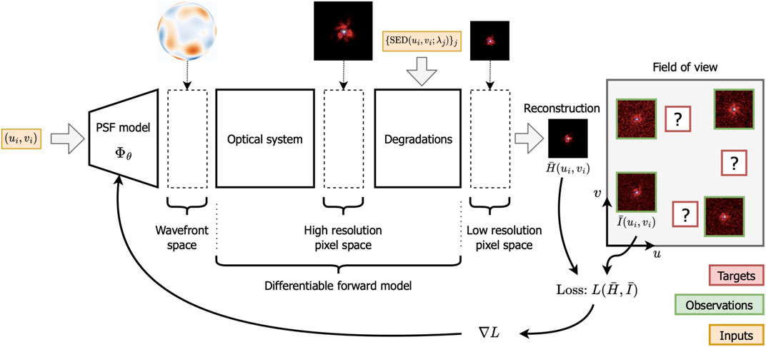
FIGURE 13. Overview of the WaveDiff approach to model the PSF with a differentiable optical forward model. Figure adapted from Liaudat et al. (2023).

Estimating the model’s parameters in the WFE space is a challenging, ill-posed inverse problem known as phase retrieval (Fienup, 1993; Fienup et al., 1993; Shechtman et al., 2015), i.e., estimating a complex signal from intensity-only observations. The optimisation problem is non-convex and non-smooth, the star observations are not very informative, and there is no guarantee that the WFE model’s structure can represent the underlying ground truth WFE. Liaudat et al. (2023) show that under the aforementioned conditions, targeting the estimation of the ground truth WFE is not the best option. The PSF model’s objective is to have a good pixel representation of the PSF. It is, therefore, possible to estimate a WFE manifold far away from the underlying WFE but very close in the pixel space. The data-driven features, the basis of the WFE manifold, are estimated with a stochastic gradient descent method widely used for estimating neural network parameters.

The WaveDiff model can handle spatial variations, super-resolve the PSF, and model chromatic variations thanks to the WFE formulation and the optical forward model, which also considers more general degradations as in Eq. 39. To the best of our knowledge and at the time of writing, this is the only data-driven PSF model that can cope with the spectral variations of the PSF. The WaveDiff shows a breakthrough in performance for data-driven PSF models in a simplified Euclid-like setting (Liaudat et al., 2023). It is flexible enough to be adapted to different space telescopes. The framework proposed shows an exciting research direction for future data-driven PSF modelling. The WaveDiff model has yet to be tested with real space-telescope observations and has to incorporate detector-level effects, which are more naturally modelled in pixel space. For more details, we refer the readers to Liaudat et al. (2023) and Liaudat (2022).

More general approaches based on differentiable optics have been recently emerging, e.g., ∂Lux ¹⁷ (Desdoigts et al., 2023). Approaches based on automatic differentiation can be useful not only for modeling the PSF but also for designing apodizing phase plate coronagraphs (Wong et al., 2021) and detector calibrations (Desdoigts et al., 2023).

5.2.9 Other PSF models

•Shapelets: Refregier (2003) proposed a framework to analyse images based on a series of localised basis functions of different shapes named shapelets and images could then be decomposed using these basis functions. Refregier and Bacon (2003) continued the work to propose the shapelet framework to be used for building shear estimates and modelling the PSF. The PSF modelling consists of decomposing the star images in the shapelet basis and then performing an interpolation of the coefficients to positions of interest. Essentially, it is an extension of the approach seen in shape interpolation. Expressing the image in shapelet coefficients allows denoising the star images and providing an easier framework for the galaxy-PSF deconvolution. However, capturing all the PSF structures in a finite expansion over analytical functions is not always possible, leading to the loss of information. Massey and Refregier (2005) extended the framework from Cartesian to polar shapelets.

•Moffatlets and Gaussianlets: Li et al. (2016) proposed two other series of basis functions to decompose the PSF named Moffatlets and Gaussianlets. They compared the PSF reconstruction using the aforementioned basis with a PCA-based method on LSST-like images. Using analytical basis functions leads to more denoised models, as expected. Nie et al. (2021a) continued the approach and forced the principal components being learnt in the PCA-like algorithm to be built using the Moffatlets basis. This choice avoids the principal components of learning noise as the Moffatlets basis avoids it. Both analyses lack a performance benchmark with a reference PSF model like PSFEx. In addition, the models’ performance is computed at the same position as the observed stars, so the models’ generalisation to other positions, a fundamental task of the PSF model, still needs to be studied.

•Fourier-based methods: Zhang (2007) proposed a Fourier-based method for directly measuring the cosmic shear, taking into account the PSF, which was further developed in several publications (Zhang, 2011; Zhang et al., 2015; Lu et al., 2017; Zhang et al., 2019). The method is based on the quadrupole moments of the galaxy images (described in detail in Section 7.2) but is measured in Fourier space. The handling of the PSF is also done in Fourier space. Lu et al. (2017) explore different interpolation approaches for the PSF in the aforementioned Fourier framework. The 2D power spectrum of the observed PSFs is interpolated to target positions. The interpolation is done pixel-by-pixel, and the best-performing method is a well-parametrised polynomial interpolation. An advantage of the Fourier interpolation is that the 2D power spectrum is automatically centred in Fourier space, simplifying the handling of images with intra-pixel shifts or, what is the same, different centroids. Another Fourier-based shear measurement method is Bayesian Fourier Domain (BFD) (Bernstein and Armstrong, 2014; Bernstein et al., 2016) built on the Bayesian formalism. However, it does not include a specific PSF model.

•Optimal transport (OT)-based methods: There exist two approaches involving OT (Peyré and Cuturi, 2019) to tackle the PSF modelling problem. Ngolè and Starck (2017) proposed to use Wasserstein barycenters as a nonlinear geometry-aware interpolation procedure of a low-dimensional embedding representation of the PSFs. Although elegant, the performance of the approach does not seem to justify its computational burden. In the comparison method, an RBF interpolation of the principal components obtained through the PCA achieves a similar performance. The performance of the PCA method is better in terms of ellipticity but slightly worse in terms of pixel error and PSF FWHM. Schmitz (2019) worked on a data-driven PSF model based on the RCA that could model the chromatic variations of the PSF through the use of Wasserstein barycenters that were previously developed by Schmitz et al. (2018). The OT-based PSF model named λRCA was compared to the RCA. The comparison showed a lower pixel and size error for λRCA, although the ellipticity error was similar or better for RCA. This method assumes that the PSF’s chromatic variation is smooth over all the passband. This assumption holds if the only chromatic effect of the PSF is due to the diffraction phenomena, which exhibits a smooth variation with the 1/λ dependence in the WFE that has already been presented in Eq. 35. However, if this is not the case and another non-smooth chromatic variation is present, currently occurring in Euclid (Venancio et al., 2016; Baron et al., 2022), there is no straightforward way to adapt the λRCA model to account for it.

•Wavefront approach: Soulez et al. (2016) proposed to model the propagation of light through the mirrors of the optical system. The PSF modelling problem is recast into the phase-retrieval problem. The article is a proof-of-concept as there are only qualitative results, and many PSF modelling difficulties remain unaddressed.

•Exploit out-of-focus images: Some instruments, like the Dark Energy Camera (DECam) (Flaugher et al., 2015), are equipped with wavefront sensors that are helpful for focus, alignment, and the adaptive optics system (AOS) (Roddier and Roddier, 1993; Roodman, 2010; Roodman, 2012). The LSST camera (LSST Science Collaboration et al., 2009) is also equipped with wavefront sensors (Manuel et al., 2010; Claver et al., 2012; Xin et al., 2015; Xin et al., 2016). Roodman et al. (2014) proposed to use the data from the wavefront sensors to constrain the optical contribution of the PSF. The work was continued by Davis et al. (2016) who proposed a wavefront-based PSF model for the DECam instrument using out-of-focus observations. The PSF model was based on Zernike polynomials fitted to out-of-focus stars, also called doughnuts, that contain considerably more wavefront information than in-focus stars. Then, a new fit is done for each exposure based on the measured quadrupole moments of the in-focus star images. It is not easy to understand at which point the quadrupole moments constrain the proposed PSF model and at which point it is the base physical wavefront measured from the out-of-focus images that are the only parts driving the performance of the model. Snyder et al. (2016) proposed using the AOS measurements to characterise atmospheric turbulence in terms of Zernike decomposition.

•Deep learning approaches: A model coined PSF-NET was proposed by Jia et al. (2020a) and is based on two convolutional neural networks (CNNs) trained jointly. One network transforms high-resolution images into low-resolution images, while the other does the opposite. The CNNs are trained in a supervised way expecting that the first network will learn a PSF manifold. However, it is unclear how the approach handles the spatial variation of the PSF, and it has not been tested for WL purposes. Jia et al. (2020b) proposed another approach for PSF modelling based on denoising auto-encoders, but the spatial variation of the PSF remains untackled. Another approach is followed by Herbel et al. (2018), where the PSF profile is modelled by a parametric function consisting of a base profile of two Moffat profiles and several parametrised distortions to increase the expressivity. A CNN is trained in a supervised manner to predict the parameters of the parametric profile from a noisy star observation. The neural network provides a good estimation of the parameters, but the spatial variation of the PSF is, again, not addressed. Having a PSF model that can model the observations is important. However, in PSF modelling for WL analysis, a crucial part is to capture the spatial variations of the PSF and that the model outputs the PSF at different positions in the FOV.

6 Desirable properties of PSF models

In the previous section, we reviewed some of the most relevant PSF models developed so far. After studying many models, we can conclude on desirable PSF model properties. The PSF model should

(a) Have an accurate modelling of the PSF light profile. This modelling is essential for any target task, as the light profile is the convolutional kernel for a given position. The smoothness and structure in the PSF profile are a consequence of the PSF being the Fourier transform, in Fraunhofer’s approximation, of a particular finite-length aperture that limits the frequency content of the PSF. This frequency limitation prevents us from having a Dirac distribution as a PSF, as it would require an infinite frequency content to build it. One difficulty is in accurately modelling the PSF’s wings or outer region, which is often below the noise level. In ground-based telescopes, the effect of the atmosphere can be interpreted as a low-pass filter for the PSF, smoothing the PSF light profile.

(b) Produce noiseless estimations of the PSF. The presence of noise in the PSF estimations is an issue for purely data-driven models, which sometimes tend to overfit noisy observations. Some regularisations have to be introduced in the PSF model parameter optimisation to avoid producing noisy PSFs. A seemingly straightforward solution to this problem is to rely on PSF models based on fixed basis functions like shapelets or Moffatlets. These models will always output denoise PSFs as their basis functions cannot reproduce the noise. However, they introduce modelling errors if they cannot accurately model the observed PSF light profiles.

(c) Capture the PSF field’s variations. It is often the case that a good quality PSF is required at the position of a certain object where no direct information about the PSF is available. The PSF model first has to capture most of the relevant information from the observations at other positions and wavelengths. Then, the model exploits this information and predicts the PSF at the required position and wavelength. The PSF model relies upon its generalisation power as it has to exploit the PSF field information from other positions.

(d) Be capable of exploiting the structure of the PSF field variations. This desired property is related to the previous point (c). An exciting approach to obtain good generalisation power is to learn the structure of the PSF field variations. This structure is a consequence of the physical properties of the telescope’s optical system. The following subsection provides a physical understanding of the PSF field structure, which imposes a certain smoothness to the variations. The spatial variations are also structured due to the atmosphere if we study the PSF field of a ground-based telescope. A data-driven PSF model should use a low-complexity representation of the PSF field, which can learn its structure and spatial variations.

(e) Handle discontinuities of the PSF field. The CCD misalignments are a source of discontinuity of the PSF’s spatial variations. The PSF field is piece-wise continuous, and the borders delimiting the discontinuity are well known as the geometry of the focal plane is accurately known. A straightforward way to handle the discontinuities is to model the PSF for each CCD independently, e.g., PSFEx. Although this is simple to implement, it limits the number of stars available to constrain the PSF model. Another more difficult but potentially more powerful approach is to build a PSF model for the entire focal plane, accounting for the focal plane discontinuities, e.g., MCCD. Another source of discontinuity is segmented mirrors, e.g., JWST’s hexagonal mirrors seen in Figure 9B.

(f) Be robust to outliers and contaminations of the star sample. Contaminations can come from the selection of stars, and the fact that the objects classified as stars are good representations of the PSF and are not small galaxies or binary stars (Kuntzer and Courbin, 2017). Outliers can come from imperfect image preprocessing where detector effects, like CTI, have not been adequately removed. In addition, the model should be robust to different observation conditions such as spatial distributions of the observed stars, SNRs, and the number of observed stars.

(g) Work appropriately with the target task. The PSF model can be exploited differently according to the target task’s objective, e.g., estimating a deconvolved object or estimating some summary statistic of the deconvolved image. The model should be developed with the task in mind, as each task might be more or less susceptible to different kinds of errors.

(h) Be fast. Upcoming surveys will be processing a vast amount of observations. Consequently, they put significant pressure on the computing time of PSF models as they have to cope with the data intake. The requirements in terms of computing time can drive many design choices in a PSF model, preventing the use of costly physical simulations.

Once the PSF model has been developed with all the aforementioned properties in mind, it is essential to validate the model’s performance. The validation should ensure that the expected performance of the model is achieved and helps to identify sources of problems and provide directions for the improvement of the model. In the next section, we give an overview of validation methods for PSF models.

7 Validation of PSF models

The validation of PSF models is a challenging problem. To derive a validation method, it would be necessary to quantify the impact of PSF modelling errors on the final objective of our analysis. We consider, as an example, a weak-lensing-based cosmological analysis, where the objective is to derive constraints on the parameter of the cosmological model under analysis. This exercise is challenging, given the analysis’ complexity and the large data volume. Nevertheless, with some simplifying assumptions, the PSF modelling requirements were set for the Euclid mission as shown in Section 7.3. In this analysis, some assumptions on the PSF shape used do not always hold for the high complexity of the PSF in a space-based mission like Euclid. Even though it is essential to derive requirements for the PSF model, these do not give much information on the nature of errors and possible problems that the PSF model has. Therefore, it is necessary to derive different diagnoses or null tests. Jarvis et al. (2016) proposed a set of null tests for the DES WL shear catalogues Science Verification, which includes the PSF model validation.

The most basic rule for any validation of the PSF models is to separate the observations in the FOV into two data sets for estimation and testing, i.e., validation, which could be 80% and 20%, respectively. The first one should be used to estimate the PSF model. The second one should help validate its performance and not be used in the PSF model estimation. This rule tests the PSF model’s generalisation power to unseen positions in the FOV. Next, we will describe the most used PSF diagnosis that will help us validate the performance of the PSF models.

7.1 Pixel-based metrics

The most straightforward diagnostic that we can think of is to compute the pixel residual of our PSF model. Once trained, the model is used to recover the PSF at test positions. We can then compute the RMSE of the pixel reconstruction residuals. The PSF model can ideally predict the observed test stars without error, and the reconstruction residual would only contain the observational noise. If we work with simulations, we can produce noiseless stars for our testing set, and the RMSE will directly indicate the pixel reconstruction error. Even though pixel-based metrics can give insight into the PSF model performance, they are not easily interpretable regarding scientific impact. Errors in the PSF core or the PSF wings can impact the observed galaxy’s estimated shape differently. With the existing methodology, it is difficult to translate a pixel-based metric into a scientifically meaningful quantity in terms of error propagation.

When working with real data, the PSF model’s validation with pixel-based metrics becomes more complicated. The different noise levels in the data can hide the pixel reconstruction error, making it difficult to compare different PSF models or even assess the performance of a single one. Liaudat et al. (2021a) proposed pixel-based reconstruction metrics for real observations. Let us denote with $I_{\text{star}}(\bar{u},\bar{v}|u_i,v_i),I_{\text{model}}(\bar{u},\bar{v}|u_i,v_i)\in {\mathbb{R}}^{p\times p}$ a test star and the predicted PSFs, respectively, at the FOV position (u _i , v _i ), where p ² is the total number of pixels in the image. To simplify the notation, we write $I(\bar{u},\bar{v}|u_i,v_i)=I_i$ . In star images, most of the PSF flux is concentrated in the centre of the square image, and the noise level can be considered constant in the image. Therefore, we can mask the image to only consider the central pixels within a given radius of R pixels and compute the pixel RMSE of the masked images. We note $\tilde{I}=I\odot M_R$ the masked image, where M _R ∈ {0,1} ^p×p is a binary mask and ⊙ is the Hadamard or element-wise product. Let us define the σ value as

$\sigma \left({\tilde{I}}_i\right)=\sigma \left(M_R\odot I_i\right)={\left(\frac{1}{{\tilde{p}}^2}\sum _{\bar{u},\bar{v}=1}^p{\left({\tilde{I}}_i\left(\bar{u},\bar{v}\right)\right)}^2\right)}^{1/2},(52)$

where ${\tilde{p}}^2$ is the number of unmasked pixels, and the sum is done on the unmasked pixel values. The first pixel metric is $Q_{p_1}$ and is defined as

$Q_{p_1}={\left({\text{Err}}^2-{\sigma }_{\text{noise}}^2\right)}^{1/2},(53)$

where

${\text{Err}}^2=\frac{1}{N_s}\sum _{i=1}^{N_s}\sigma {\left({\tilde{I}}_{\text{star},i}-{\tilde{I}}_{\text{model},i}\right)}^2,\text{and}{\sigma }_{\text{noise}}^2=\frac{1}{N_s}\sum _{i=1}^{N_s}\sigma {\left({\tilde{I}}_{\text{star},i}^{*}\right)}^2,(54)$

where the general noise standard deviation, σ _noise, is computed from the pixels on the outer region of the test stars, i.e., $\widetilde{I^{*}}$ , which we define as $\widetilde{I^{*}}=I_{\text{star}}\odot M_R^{*}$ , where $M_R^{*}$ is such that $M_R^{*}+M_R=1_{p\times p}$ . Subtracting our estimated model, I _model, from an observed star, I _star, should lead to a residual map containing only noise if the model is perfect. The probability of having our model correlated with the noise is minimal. Therefore, the method with the smallest $Q_{p_1}$ can be considered the best from the $Q_{p_1}$ point of view.

The next two metrics, $Q_{p_2}$ and $Q_{p_3}$ , help quantify the model noise. Let us define ${\sigma }_{\text{model},i}^2={[\sigma {({\tilde{I}}_{\text{star},i}-{\tilde{I}}_{\text{model},i})}^2-\sigma {({\tilde{I}}_{\text{star},i}^{*})}^2]}_{+}$ , where the operator [⋅]₊ sets to zero negative values. Then, both metrics are defined as follows:

$Q_{p_2}={\left(\frac{1}{N_s}\sum _{i=1}^{N_s}{\sigma }_{\text{model},i}^2\right)}^{1/2},Q_{p_3}={\left(\frac{1}{N_s}\frac{1}{N_s}\sum _{i=1}^{N_s}{\left({\sigma }_{\text{model},i}^2-Q_{p_2}^2\right)}^2\right)}^{1/4}.(55)$

The $Q_{p_2}$ metric represents the modelling error expectation for a given star, and the $Q_{p_3}$ metric indicates the fluctuation of the modelling error. A perfect PSF model would give values close to zero for the three metrics. We have assumed that there is no background contamination in the observed test stars or that it has been removed.

7.1.1 Chromatic PSF models

Some applications or analyses require a chromatic PSF model, and it is essential to validate the chromaticity of the PSF model. This monochromatic validation means validating the PSF at every single wavelength or validating the monochromatic PSF before it is integrated into the instrument’s passband. A PSF model with a good performance in reproducing the polychromatic stars does not necessarily have a good monochromatic performance. Supposing that is the case and even if the spectra of the different objects are known in advance, the PSF errors will be more significant when used with objects with considerably different spectra, e.g., galaxies. Chromatic PSF models will generally be required if the observing instrument has a wide passband, e.g., the Euclid’s VIS instrument passband goes from 550 nm to 900 nm. The pixel RMSE can be computed for monochromatic PSFs in the passband as done in Liaudat et al. (2023). However, it is cumbersome to validate with real data as we usually do not have access to the monochromatic PSFs of the instrument under study. Consequently, the monochromatic validation might only be possible with simulations.

7.2 Moment-based metrics

Weak gravitational lensing analyses are interested in measuring the shape of galaxies as the measured ellipticity is an estimator of the shear. Cosmologists have developed formulations to relate the PSF errors, expressed in terms of shape and size metrics (Massey et al., 2012), to the cosmological parameters of interest (Cropper et al., 2013). Therefore, it seems natural to have diagnosis metrics based on the ellipticity and size of the PSF. These metrics are determined using the moments of the polychromatic observation $\bar{I}[u,v]$ . Following Hirata and Seljak (2003), we redefine the image moments that we will use in practice, which include a weight function as follows:

$<\mu >=\frac{\int \mu \bar{I}\left(\bar{u},\bar{v}\right)w\left(\bar{u},\bar{v}\right)\text{d}\bar{u}\text{d}\bar{v}}{\int \bar{I}\left(\bar{u},\bar{v}\right)w\left(\bar{u},\bar{v}\right)\text{d}\bar{u}\text{d}\bar{v}},(56)$

$M_{\mu \nu }=\frac{\int \bar{I}\left(\bar{u},\bar{v}\right)\left(\mu -<\mu >\right)\left(\nu -<\nu >\right)w\left(\bar{u},\bar{v}\right)\text{d}\bar{u}\text{d}\bar{v}}{\int \bar{I}\left(\bar{u},\bar{v}\right)w\left(\bar{u},\bar{v}\right)\text{d}\bar{u}\text{d}\bar{v}},(57)$

where $\mu ,\nu \in \{\bar{u},\bar{v}\}$ , $<\mu >$ denotes the mean of μ, and $w(\bar{u},\bar{v})$ is a weight function that helps in noisy settings. The weight function is also useful to compute the moments from diffraction-limited PSFs, e.g., an Airy profile, as they prevent the integral from diverging due to the wings of the PSF. Eq. 56 defines the first-order moments, while Eq. 57 defines the second-order moments. The ellipticities, or shape metrics, are defined as

$e=e_1+\text{i}{e}_2=\frac{\left(M_{\bar{u}\bar{u}}-M_{\bar{v}\bar{v}}\right)+\text{i}2M_{\bar{u}\bar{v}}}{M_{\bar{u}\bar{u}}+M_{\bar{v}\bar{v}}},(58)$

where i is the imaginary unit, and the size metric is defined as

$R^2=T=M_{\bar{u}\bar{u}}+M_{\bar{v}\bar{v}}.(59)$

One widely used method to estimate these metrics is the adaptive moment algorithm from GalSim’s HSM (Hirata and Seljak, 2003; Mandelbaum et al., 2005). The adaptive moment algorithm measurement provides σ as size, which relates to the aforementioned size metric as R ² = 2σ ². The measurements are carried out on well-resolved polychromatic images. If the observations are undersampled, as is the case for Euclid, a super-resolution step is required for the model. Gillis et al. (2020) proposed alternative metrics, based on the image moments, that target the validation of space-based PSFs with emphasis on the HST PSF.

The measurements of the shape parameters based on the image moments are susceptible to image noise. If we are working with real data, we do not have access to ground truth images and are obliged to work with noisy observations. Therefore, we have to average over many objects in order to conclude from the different diagnostics. We continue by presenting different moment-based metrics.

7.2.1 Shape RMSE

We start with a set of test stars and their corresponding PSF estimations. Then, the most direct moment-based metric is to compute the RMSE of the ellipticities and size residuals between the observations and model prediction. However, this metric could be more insightful as it does not provide any information about the composition of the residuals and the estimation biases involved.

7.2.2 meanShapes

A useful diagnostic is to compute the spatial distribution of the ellipticities and size residuals, which we coin meanShapes. For an example, see Figure 14. This diagnostic allows us to inspect if there are spatial correlations in the shape and size residuals, indicating that the PSF model is not capturing certain spatial variations from the PSF field. In order to have a finely sampled distribution, we have to average over many exposures, as the available stars from a single exposure are not enough to observe patterns. The shape measurements are also noisy, therefore averaging over many exposures allows us to smooth out the residuals and observe systematic modelling errors. In practice, we divide the focal plane into several spatial bins, consider several exposures, and then the value of each bin is built by averaging the residuals of all the stars within that bin. A ground-based survey allows us to average the ellipticity contribution of the atmosphere (Heymans et al., 2012), as it can be considered a random field with a zero mean. Then, the observed ellipticity distribution over the focal plane is due to the telescope’s optical system that is consistent in every exposure. It is also possible to plot the same spatial distribution but observe the positions of the stars. Such a plot will help observe if there are regions of stellar under-density that could eventually affect the PSF model.

FIGURE 14

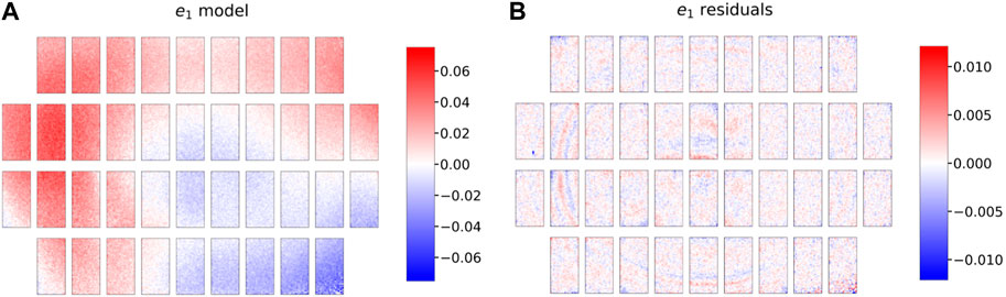
FIGURE 14. meanShapes plots showing the first component of the ellipticity of the PSF model (A) and of its residuals with the observed stars (B). The figure shows the 40-CCD mosaic from the MegaCam instrument’s focal plane at the Canada–France–Hawaii Telescope. Figure reproduced from Guinot et al. (2022).

We have assumed that the ellipticities and sizes are good descriptors, or summary statistics, of the PSF shape. If this is not the case, the diagnostic could be extended with more accurate descriptors.

7.2.3 ρ-statistics

Rowe (2010) proposed to compute the auto- and cross-correlations of the ellipticities and their residuals as a diagnostic. The diagnostic was then expanded by Jarvis et al. (2016) to a combination of ellipticities, sizes, and residuals. The ρ-statistics are helpful in identifying PSF modelling biases and detecting the scales at which it most affects the weak-lensing analysis. Following Jarvis et al. (2016), we define the ρ-statistics as follows:

${\rho }_1\left(\theta \right)=⟨\delta e_{\text{PSF}}^{*}\left({\mathit{\theta }}^{\prime }\right)\delta e_{\text{PSF}}\left({\mathit{\theta }}^{\prime }+\mathit{\theta }\right)⟩,(60)$

${\rho }_2\left(\theta \right)=⟨e_{\text{PSF}}^{*}\left({\mathit{\theta }}^{\prime }\right)\delta e_{\text{PSF}}\left({\mathit{\theta }}^{\prime }+\mathit{\theta }\right)⟩,(61)$

${\rho }_3\left(\theta \right)=⟨\left(e_{\text{PSF}}^{*}\frac{\delta R_{\text{PSF}}^2}{R_{\text{PSF}}^2}\right)\left({\mathit{\theta }}^{\prime }\right)\left(e_{\text{PSF}}\frac{\delta R_{\text{PSF}}^2}{R_{\text{PSF}}^2}\right)\left({\mathit{\theta }}^{\prime }+\mathit{\theta }\right)⟩,(62)$

${\rho }_4\left(\theta \right)=⟨\delta e_{\text{PSF}}^{*}\left({\mathit{\theta }}^{\prime }\right)\left(e_{\text{PSF}}\frac{\delta R_{\text{PSF}}^2}{R_{\text{PSF}}^2}\right)\left({\mathit{\theta }}^{\prime }+\mathit{\theta }\right)⟩,(63)$

${\rho }_5\left(\theta \right)=⟨e_{\text{PSF}}^{*}\left({\mathit{\theta }}^{\prime }\right)\left(e_{\text{PSF}}\frac{\delta R_{\text{PSF}}^2}{R_{\text{PSF}}^2}\right)\left({\mathit{\theta }}^{\prime }+\mathit{\theta }\right)⟩,(64)$

where * denotes complex conjugation, θ and θ ′ denote sky positions, θ denotes the modulus of θ , and δ denotes the residual error that can be computed as δe _PSF = e _PSF − e _star in case of PSF ellipticity. Suppose that the ellipticities are random fields that are isotropic and statistically homogenous. In such a case, we can compute the correlation ρ( θ , θ ′) as ρ(| θ − θ ′|) = ρ(θ), using the modulus θ. This choice means that we are assuming translational and rotational symmetry, a consequence of the cosmological principle. We define several θ bins in a logarithmic scale, corresponding to ln θ − Δ ln θ/2 < ln θ _ij < ln θ + Δ ln θ/2, where θ _ij = | θ _i − θ _j | is the distance between two objects at θ _i and θ _j . Consequently, the correlation function at θ can be computed using the following unbiased estimator of ρ:

$\widehat{\rho }\left(\theta \right)=\frac{{\sum }_{i,j}{w}_i{w}_j{e}_i^{\text{A}*}{e}_j^{\text{B}}}{{\sum }_{i,j}{w}_i{w}_j},(65)$

where we are computing, as an example, the correlation of two ellipticities e ^A and e ^B, and the weights depend on the SNR of the ellipticity measurements. We carry out the weighted sum over the pairs of objects within each bin.

The ρ-statistics are interesting as they can be propagated to the shear two-point correlation function (2PCF) (Kilbinger, 2015), which allows for studying the properties of the weak-lensing convergence field. Following Jarvis et al. (2020), we include the PSF errors into the shear 2PCF, making the ρ-statistics appear, and then express the systematic error in the shear 2PCF.

7.2.4 Other shape metrics

Another shape metric that gives insights into the performance of the PSF model in a weak-lensing analysis is the PSF leakage α from Jarvis et al. (2016). It is related to the linear modelling of the shear bias and where it has been decomposed into a multiplicative bias and an additive bias further decomposed into PSF-dependent (leakage) and PSF-independent terms. The PSF leakage helps quantify how the PSF affects the shear estimation through shape measurement. It measures the leakage of the PSF shape to the galaxy shapes.

7.3 Weak lensing: PSF error propagation and PSF requirements definition

The pioneers in the PSF error propagation for WL were Paulin-Henriksson et al. (2008), followed by Massey et al. (2012). The proposed framework is based on the second-order moments of the images, i.e., complex ellipticity e and size R ². It expresses how the PSF, or some other effect, affects the observed ellipticity and size. Let us consider the effect of the PSF on the unweighted moments from Eqs 58, 59 where unweighted represents computing Eqs 56, 57 without the w weight function. Then, we obtain

$e_{\text{obs}}=e_{\text{gal}}+\frac{R_{\text{PSF}}^2}{R_{\text{PSF}}^2+R_{\text{gal}}^2}\left(e_{\text{PSF}}-e_{\text{gal}}\right)\text{and}{R}_{\text{obs}}^2=R_{\text{gal}}^2+R_{\text{PSF}}^2,(66)$

where the subscript _obs refers to the quantity measured to the observed galaxy, the subscript _gal refers to the intrinsic quantity of the galaxy, and _PSF refers to the quantity measured to the PSF. There are intrinsic assumptions in Eq. 66, that the observational model is I _obs = I _gal*H _PSF, and that all the moments are well-defined. Then, Eq. 66 can be rewritten to express the quantity of interest in weak lensing, the intrinsic galaxy ellipticity, as follows:

$e_{\text{gal}}=\frac{e_{\text{obs}}{R}_{\text{obs}}^2-e_{\text{PSF}}{R}_{\text{PSF}}^2}{R_{\text{obs}}^2-R_{\text{PSF}}^2}.(67)$

The error propagation consists of expanding the previous equation in a first-order Taylor series with respect to the quantities of interest. In this case, it will be the shape and size of the PSF, and the propagation is given by

${\widehat{e}}_{\text{gal}}\approx e_{\text{gal}}+\frac{\partial e_{\text{gal}}}{\partial \left(R_{\text{PSF}}^2\right)}\delta \left(R_{\text{PSF}}^2\right)+\frac{\partial e_{\text{gal}}}{\partial e_{\text{PSF}}}\delta e_{\text{PSF}},(68)$

where δ refers to errors in the model with respect to the ground truth. It is straightforward to compute the partial derivatives in Eq. 68 from Eq. 67. We then obtain the following expression:

${\widehat{e}}_{\text{gal}}\approx e_{\text{gal}}\left(1+\frac{\delta \left(R_{\text{PSF}}^2\right)}{R_{\text{gal}}^2}\right)-\left(\frac{R_{\text{PSF}}^2}{R_{\text{gal}}^2}\delta e_{\text{PSF}}+\frac{\delta \left(R_{\text{PSF}}^2\right)}{R_{\text{gal}}^2}{e}_{\text{PSF}}\right).(69)$

The previous ellipticity estimator can be used to obtain a shear estimator assuming that the intrinsic galaxy distribution has a zero mean. The estimator can then be used in the linear shear bias parametrization from Jarvis et al. (2016). At this point, we can express the additive and multiplicative biases as a function of the elements from Eq. 69. This analysis shows us that the multiplicative bias is related to the size of the PSF with its estimation error and the size of the galaxy. The result is as expected if we pay attention to the first term of Eq. 69.

This framework allows us to consider different types of errors. Massey et al. (2012) use it to include errors due to non-convolutional detector effects, imperfect shape measurement, and the fact that the shape measurement method used weighted, i.e., Eq. 57, instead of unweighted moments. The procedure consists of adding the desired effect to the galaxy ellipticity expression, Eq. 67, and then adding their corresponding partial derivatives to the Taylor expansion seen in Eq. 68. Cropper et al. (2013) use this formalism to derive requirements for a WL mission in space. The aforementioned framework was used to derive the current PSF model requirements for the Euclid space mission (Laureijs et al., 2011).

The previous formalism is based on unweighted moments. However, in practice, the moments are always computed from noisy images using a compact weight function to ensure that the measurement yields significant results. Melchior et al. (2011) and Melchior and Viola (2012) showed that using a weight function mixes the image’s moments. Consequently, the second-order moments are affected by higher-order moments even in the absence of noise, thus exposing the Paulin-Henriksson et al. (2008) framework’s fundamental limitations. Schmitz et al. (2020) then noted and verified empirically in an Euclid-like scenario that the propagation is based on second-order moments of the PSF, which do not accurately describe the shape of a space-based PSF. A perfect second-order moment estimation of the PSF would have a zero shear bias contribution in the formalism described. However, the PSF’s higher moments error (HME) will impact the shear biases and are not considered in the framework proposed by Paulin-Henriksson et al. (2008). The higher the contribution of the HME to the PSF, the more significant the deviations are. A space mission like Euclid will have a PSF close to the diffraction limit, i.e., its shape will be complex and not well described by a Gaussian (or by its second-order moments). As a space PSF is not well described by second-order moments, the previous requirements should be used with caution. The LSST collaboration, concerned with the previous issue, studied the contribution to systematic biases of the HME of the PSF model on the shear measurement (Zhang et al., 2021; Zhang et al., 2022). Zhang et al. (2021) showed that the HME of the PSF model might be a significant source of systematics in upcoming WL analyses. Zhang et al. (2022) studied the impact of moments from the third to sixth order on the cosmological parameter inference, concluding that the HME of PSF models like PSFEx and PIFF should be reduced for future surveys like LSST if the WL analysis is to remain unchanged.

The use and adoption of automatic differentiable (Baydin et al., 2017) models could make a significant contribution to error propagation. The derivatives of the target estimators with respect to the model’s parameters, or intermediate products with physical meaning, would be available. This fact allows us to consider more complex scenarios than the one seen in Eq. 66, as we would not require explicitly writing the equations nor their derivatives. A differentiable forward model should be enough to describe how the PSF interacts with the target task.

8 Conclusion

This review gives an overview of point spread function (PSF) modelling for astronomical telescopes, emphasising cosmological analyses based on weak gravitational lensing. This application sets the tightest constraints on the PSF models and has driven much of the last progress in PSF models. The development of new instruments and telescopes seeking higher precision and accuracy requires more powerful PSF models to keep up with the reduction of other sources of errors. We differentiate two scenarios that fundamentally change how the PSF is modelled: the ground- and space-based telescopes. The main difference is the atmosphere, how it affects the observations, and how challenging it is to build an atmospherical physical model that can be exploited in a reasonable amount of time. The difficulty of handling the temporal integration of a representative atmospherical model fosters the use of purely data-driven PSF models built in the pixel space for ground-based telescopes. The stability of space-based telescopes allows for exploiting models more physically based on the wavefront.

The optics fundamentals to properly define the PSF and understand its effect on the underlying imaged object are not often introduced in PSF modelling articles. One of our goals was to solve this issue by providing a concise yet comprehensive introduction to optical principles. The provided optical background should cover most of the available PSF models and motivate the general observational model that we have proposed. This observational model can be further simplified and adapted to different use cases, which include ground or space telescopes. We described several assumptions that might not always hold. After describing how the PSF affects our observations, we presented an extended list of the leading optical- and detector-level contributors to the PSF field. These contributors are the sources of PSF’s spatial, spectral, and temporal variations in addition to its morphology. A detailed description of the atmospheric contribution based on phase screens was presented. We then gave a brief description of the most relevant PSF models.

The PSFEx model has been successful in modelling the PSF for several surveys with its robust and fast implementation. However, the next-generation telescopes set higher PSF requirements, demanding novel models to achieve such performances. Recent models target upcoming telescopes, e.g., the Vera C. Rubin observatory and the Euclid telescope and Roman Space Telescope. These models are continuously being developed, and they push forward the capabilities of PSF modelling. A common bottleneck for these is the computing time required to estimate the model from observations. It is unclear if the solution can be achieved through better software implementations that exploit parallel computing architectures or better-performing programming languages. A refactoring of the methods allowing for simplifications that accelerate calculations might be required, or even both approaches. One big challenge of PSF modelling is to build fast yet powerful models.

Another challenge is to include complex effects and contributions that cannot be directly constrained from the observations into the PSF model. These contributions can be modelled with simulations and obtained from complementary observations or instrument characterisations. However, this complementary information will not precisely match the state of the telescope during the imaging procedure due to several reasons, e.g., changes in the telescope, measurement errors, and imperfect modelling. The better way to correct this information and adapt it to real observations has to be further studied.

The validation of PSF models from real observations is a challenging subject that requires further development, as access to the ground truth PSF field is unavailable. Although some validation methods exist, they are generally not very informative or are based on second-order moments that are not well-suited to describe diffraction-limited PSFs. We have presented the error propagation of a galaxy-shape measurement, where several limitations were exposed. Current error propagation methods have simplifying assumptions, e.g., the PSF is well described by its quadrupole moments that do not hold anymore with recent and upcoming telescopes. Further development of these methods is required to define realistic PSF model requirements and study how PSF modelling errors affect the target task.

Author contributions

TL coordinated the entire effort, produced the figures, and wrote the text. J-LS and MK provided valuable comments and feedback on the different sections of the article. All authors contributed to the article and approved the submitted version.

Funding

This work was partially funded by the TITAN ERA Chair project (Contract No. 101086741) within the Horizon Europe Framework Programme of the European Commission. This work is also partially supported by EPSRC (grant number EP/W007673/1).

Acknowledgments

Part of this review has been adapted from the PhD thesis (Liaudat, 2022). The authors acknowledge and resume in the following list the open-source simulating and modelling software mentioned in this review:

•GalSim (Rowe et al., 2015): github.com/GalSim-developers/GalSim

•WebbPSF (Perrin et al., 2014): github.com/spacetelescope/webbpsf

•PhoSim (Peterson et al., 2015): bitbucket.org/phosim/phosim_release/wiki/Home

•WaveDiff (Liaudat et al., 2023): github.com/CosmoStat/wf-psf

•ShapePipe (Farrens, S. et al., 2022): github.com/CosmoStat/shapepipe

•PIFF (Jarvis et al., 2020): github.com/rmjarvis/Piff

•MCCD (Liaudat et al., 2021a): github.com/CosmoStat/mccd

•RCA (Ngolè et al., 2016; Schmitz et al., 2020): github.com/CosmoStat/rca

•PSFEx (Bertin, 2011): github.com/astromatic/psfex

•Tiny Tim (Krist et al., 2011): github.com/spacetelescope/tinytim

•Photutils (Bradley et al., 2022): github.com/astropy/photutils

•∂Lux (Desdoigts et al., 2023): github.com/LouisDesdoigts/dLux

•psf-weather-station: github.com/LSSTDESC/psf-weather-station.

Conflict of interest

The authors declare that the research was conducted in the absence of any commercial or financial relationships that could be construed as a potential conflict of interest.

Publisher’s note

All claims expressed in this article are solely those of the authors and do not necessarily represent those of their affiliated organizations, or those of the publisher, the editors, and the reviewers. Any product that may be evaluated in this article, or claim that may be made by its manufacturer, is not guaranteed or endorsed by the publisher.

Footnotes

¹ The binomial expansion is given by $\sqrt{1+b}=1+\frac{1}{2}b-\frac{1}{8}{b}^2+\cdots$ .

² Refraction refers to the change of direction in the propagation of a wave passing from one medium to another. Most of the wave energy is transmitted to the new medium. Reflection refers to the abrupt change of direction of the wave propagation due to a boundary between mediums. In this last case, most of the oncoming wave energy remains in the same medium.

³ The filter curves can be downloaded from the Spanish Virtual Observatory (SVO) webpage, http://svo2.cab.inta-csic.es/svo/theory/fps/index.php.

⁴ https://www.cfht.hawaii.edu/Science/CFIS/

⁵ github.com/LSSTDESC/psf-weather-station

⁶ bitbucket.org/phosim/phosim_release/wiki/Home

⁷ github.com/GalSim-developers/GalSim

⁸ github.com/spacetelescope/tinytim

⁹ github.com/astropy/photutils

¹⁰ github.com/spacetelescope/webbpsf

¹¹ github.com/astromatic/psfex

¹² github.com/CosmoStat/rca

¹³ In the signal processing community, a dictionary is a collection of templates, or basic elements, used to decompose a signal.

¹⁴ github.com/CosmoStat/mccd

¹⁵ github.com/rmjarvis/Piff

¹⁶ github.com/CosmoStat/wf-psf

¹⁷ github.com/LouisDesdoigts/dLux

References

Akeson, R., Armus, L., Bachelet, E., Bailey, V., Bartusek, L., Bellini, A., et al. (2019). The wide field infrared survey telescope: 100 hubbles for the 2020s. arXiv e-prints , arXiv:1902.05569. doi:10.48550/arXiv.1902.05569

CrossRef Full Text | Google Scholar

Anderson, J. (2016). Empirical models for the WFC3/IR PSF. Tech. Rep.

Google Scholar

Anderson, J., and King, I. R. (2000). Toward high-precision astrometry with wfpc2. i. deriving an accurate point-spread function. Publ. Astronomical Soc. Pac. 112, 1360. doi:10.1086/316632

CrossRef Full Text | Google Scholar

Anderson, J., and King, I. R. (2006). PSFs, photometry, and astronomy for the ACS/WFC. Tech. Rep.

Google Scholar

Angeli, G. Z., Xin, B., Claver, C., MacMartin, D., Neill, D., Britton, M., et al. (2014). “Real time wavefront control system for the large synoptic survey telescope (LSST),” in Proceeding volume 9150 modeling, systems engineering, and project management for astronomy VI. Editors G. Z. Angeli, and P. Dierickx (Society of Photo-Optical Instrumentation Engineers SPIE), 91500H. doi:10.1117/12.2055390

CrossRef Full Text | Google Scholar

Antilogus, P., Astier, P., Doherty, P., Guyonnet, A., and Regnault, N. (2014). The brighter-fatter effect and pixel correlations in CCD sensors. J. Instrum. 9, C03048. doi:10.1088/1748-0221/9/03/c03048

CrossRef Full Text | Google Scholar

Baer, R. L. (2006). “A model for dark current characterization and simulation,” in Proceedings volume 6068, sensors, cameras, and systems for scientific/industrial applications VII; 606805. Editor M. M. Blouke (International Society for Optics and Photonics SPIE), 37–48. doi:10.1117/12.639844

CrossRef Full Text | Google Scholar

Baron, M., Sassolas, B., Frugier, P.-A., Venancio, L. M. G., Amiaux, J., Castelnau, M., et al. (2022). “Measurement and modelling of the chromatic dependence of a reflected wavefront on the Euclid space telescope dichroic mirror,” in Space telescopes and instrumentation 2022: optical, infrared, and millimeter wave. Editors L. E. Coyle, S. Matsuura, and M. D. Perrin (International Society for Optics and Photonics SPIE), 12180, 121804V. doi:10.1117/12.2630072

CrossRef Full Text | Google Scholar

Basden, A., Tubbs, B., and Mackay, C. (2004). “L3ccd’s: low readout noise ccds in astronomy,” in Scientific detectors for astronomy. Editors P. Amico, J. W. Beletic, and J. E. Beletic (Dordrecht: Springer Netherlands), 599–602.

CrossRef Full Text | Google Scholar

Baydin, A. G., Pearlmutter, B. A., Radul, A. A., and Siskind, J. M. (2017). Automatic differentiation in machine learning: a survey. J. Mach. Learn. Res. 18, 5595–5637.

Google Scholar

Beamer, B., Nomerotski, A., and Tsybychev, D. (2015). A study of astrometric distortions due to “tree rings” in CCD sensors using LSST Photon Simulator. J. Instrum. 10 (05), C05027. doi:10.1088/1748-0221/10/05/C05027

CrossRef Full Text | Google Scholar

Beck, A., and Teboulle, M. (2009). A fast iterative shrinkage-thresholding algorithm for linear inverse problems. SIAM J. Img. Sci. 2, 183–202. doi:10.1137/080716542

CrossRef Full Text | Google Scholar

Beckers, J. M. (1993). Adaptive optics for astronomy: principles, performance, and applications. Annu. Rev. Astronomy Astrophysics 31, 13–62. doi:10.1146/annurev.aa.31.090193.000305

CrossRef Full Text | Google Scholar

Bély, P., Hasan, H., and Miebach, M. (1993). Orbital focus variations in the hubble space telescope. Tech. Rep.

Google Scholar

Beran, M. J., and Parrent, G. B. (1964). “Theory of partial coherence,” in Prentice-Hall International series in physics (Englewood Cliffs, N.J: Prentice-Hall).

Google Scholar

Bernstein, G. (2002). Advanced exposure-time calculations: undersampling, dithering, cosmic rays, astrometry, and ellipticities. Publ. Astronomical Soc. Pac. 114, 98–111. doi:10.1086/337997

CrossRef Full Text | Google Scholar

Bernstein, G. M., and Armstrong, R. (2014). Bayesian lensing shear measurement. Mon. Notices R. Astronomical Soc. 438, 1880–1893. doi:10.1093/mnras/stt2326

CrossRef Full Text | Google Scholar

Bernstein, G. M., Armstrong, R., Krawiec, C., and March, M. C. (2016). An accurate and practical method for inference of weak gravitational lensing from galaxy images. Mon. Notices R. Astronomical Soc. 459, 4467–4484. doi:10.1093/mnras/stw879

CrossRef Full Text | Google Scholar

Bertin, E., and Arnouts, S. (1996). Sextractor: software for source extraction. Astron. Astrophys. Suppl. Ser. 117, 393–404. doi:10.1051/aas:1996164

CrossRef Full Text | Google Scholar

Bertin, E. (2011). “Automated morphometry with SExtractor and PSFEx,” in Astronomical data analysis software and systems XX. Editors I. N. Evans, A. Accomazzi, D. J. Mink, and A. H. Rots (Astronomical Society of the Pacific Conference Series), 442, 435.

Google Scholar

Beuzit, J.-L., Vigan, A., Mouillet, D., Dohlen, K., Gratton, R., Boccaletti, A., et al. (2019). Sphere: the exoplanet imager for the very large telescope. A&A 631, A155. doi:10.1051/0004-6361/201935251

CrossRef Full Text | Google Scholar

Biesiadzinski, T., Lorenzon, W., Newman, R., Schubnell, M., Tarlé, G., and Weaverdyck, C. (2011). Measurement of reciprocity failure in near-infrared detectors. Publ. Astronomical Soc. Pac. 123, 179. doi:10.1086/658282

CrossRef Full Text | Google Scholar

Bohlin, R. C., Lindler, D. J., and Riess, A. (2005). Grism sensitivities and apparent non-linearity. Tech. Rep.

Google Scholar

Born, M., and Wolf, E. (1999). Principles of optics: electromagnetic theory of propagation, interference and diffraction of light. 7 edn. Cambridge: Cambridge University Press. doi:10.1017/CBO9781139644181

CrossRef Full Text | Google Scholar

Bosch, J., Armstrong, R., Bickerton, S., Furusawa, H., Ikeda, H., Koike, M., et al. (2017). The Hyper Suprime-Cam software pipeline. Publ. Astronomical Soc. Jpn. 70. doi:10.1093/pasj/psx080.S5

CrossRef Full Text | Google Scholar

Bradley, L., Sipőcz, B., Robitaille, T., Tollerud, E., Vinícius, Z., Deil, C., et al. (2022). astropy/photutils: 1.5.0. Zenodo. doi:10.5281/zenodo.6825092

CrossRef Full Text | Google Scholar

Breckinridge, J. B., Lam, W. S. T., and Chipman, R. A. (2015). Polarization aberrations in astronomical telescopes: the point spread function. Publ. Astronomical Soc. Pac. 127, 445. doi:10.1086/681280

CrossRef Full Text | Google Scholar

Breckinridge, J. B., and Wood, H. J. (1993). Space optics: an introduction by the editors. Appl. Opt. 32, 1677–1680. doi:10.1364/AO.32.001677

PubMed Abstract | CrossRef Full Text | Google Scholar

Burke, C. J., Peterson, J. R., Egami, E., Leisenring, J. M., Sembroski, G. H., and Rieke, M. J. (2019). PhoSim-NIRCam: photon-by-photon image simulations of the James Webb Space Telescope’s near-infrared camera. J. Astron. Telesc. Instrum. Syst. 5 (3), 1–14. doi:10.1117/1.JATIS.5.3.038002

CrossRef Full Text | Google Scholar

Carlsten, S. G., Strauss, M. A., Lupton, R. H., Meyers, J. E., and Miyazaki, S. (2018). Wavelength-dependent PSFs and their impact on weak lensing measurements. Monthly Notices of the Royal Astronomical Society.

CrossRef Full Text | Google Scholar

Chang, C., Marshall, P. J., Jernigan, J. G., Peterson, J. R., Kahn, S. M., Gull, S. F., et al. (2012). Atmospheric point spread function interpolation for weak lensing in short exposure imaging data. Monthly Notices of the Royal Astronomical Society), 427 (3). 2572–2587. doi:10.1111/j.1365-2966.2012.22134.x

CrossRef Full Text | Google Scholar

Cheng, J., and Peterson, J. P. (2017). Strong gravitational lens modeling of the cosmic horseshoe and photon simulation of DECam images. Indiana: Purdue University (10266501), 159.

Google Scholar

Claver, C. F., Chandrasekharan, S., Liang, M., Xin, B., Alagoz, E., Arndt, K., et al. (2012). “Prototype pipeline for LSST wavefront sensing and reconstruction,” in Ground-based and airborne telescopes IV. Editors L. M. Stepp, R. Gilmozzi, and H. J. Hall (International Society for Optics and Photonics SPIE), 8444. 84444P. doi:10.1117/12.926472

CrossRef Full Text | Google Scholar

Condat, L. (2013). A primal–dual splitting method for convex optimization involving lipschitzian, proximable and linear composite terms. J. Optim. Theory Appl. 158, 460–479.

CrossRef Full Text | Google Scholar

Coulton, W. R., Armstrong, R., Smith, K. M., Lupton, R. H., and Spergel, D. N. (2018). Exploring the brighter-fatter effect with the hyper suprime-cam. ApJ 155, 258.

CrossRef Full Text | Google Scholar

Crew, H., Huygens, C., Young, T., Fresnel, A. J., and Arago, F. (1900). The wave theory of light: memoirs of huygens, young and fresnel. New York: American Book Co.

Google Scholar

Cropper, M., Hoekstra, H., Kitching, T., Massey, R., Amiaux, J., Miller, L., et al. (2013). Defining a weak lensing experiment in space. MNRAS 431, 3103–3126.

CrossRef Full Text | Google Scholar

Davies, R., and Kasper, M. (2012). Adaptive optics for astronomy. Annu. Rev. Astronomy Astrophysics 50, 305–351. doi:10.1146/annurev-astro-081811-125447

CrossRef Full Text | Google Scholar

Davis, C. P., Rodriguez, J., and Roodman, A. (2016). “Wavefront-based PSF estimation,” in Ground-based and airborne telescopes VI. Editors H. J. Hall, R. Gilmozzi, and H. K. Marshall (International Society for Optics and Photonics SPIE), 9906, 2156–2168. doi:10.1117/12.2233366

CrossRef Full Text | Google Scholar

de Vries, W. H., Olivier, S. S., Asztalos, S. J., Rosenberg, L. J., and Baker, K. L. (2007). Image ellipticity from atmospheric aberrations. Astrophysical J. 662, 744–749. doi:10.1086/517873

CrossRef Full Text | Google Scholar

Debarnot, V., Escande, P., Mangeat, T., and Weiss, P. (2021a). Learning low-dimensional models of microscopes. IEEE Trans. Comput. Imaging 7, 178–190. doi:10.1109/TCI.2020.3048295

CrossRef Full Text | Google Scholar

Debarnot, V., Escande, P., Mangeat, T., and Weiss, P. (2021b). “Modelling a microscope as low dimensional subspace of operators,” in 2020 28th European signal processing conference (EUSIPCO), 765–769. doi:10.23919/Eusipco47968.2020.9287603

CrossRef Full Text | Google Scholar

Desdoigts, L., Pope, B. J. S., Dennis, J., and Tuthill, P. G. (2023). Differentiable optics with ∂Lux: I—deep calibration of flat field and phase retrieval with automatic differentiation. J. Astronomical Telesc. Instrum. Syst. 9, 028007. doi:10.1117/1.JATIS.9.2.028007

CrossRef Full Text | Google Scholar

Donlon, K., Ninkov, Z., and Baum, S. (2018). Point-spread function ramifications and deconvolution of a signal dependent blur kernel due to interpixel capacitive coupling. Publ. Astronomical Soc. Pac. 130, 074503. doi:10.1088/1538-3873/aac261

CrossRef Full Text | Google Scholar

Dougherty, G., and Kawaf, Z. (2001). The point spread function revisited: image restoration using 2-d deconvolution. Radiography 7, 255–262. doi:10.1053/radi.2001.0341

CrossRef Full Text | Google Scholar

Ellerbroek, B. L. (2002). Efficient computation of minimum-variance wave-front reconstructors with sparse matrix techniques. J. Opt. Soc. Am. A 19, 1803–1816. doi:10.1364/JOSAA.19.001803

PubMed Abstract | CrossRef Full Text | Google Scholar

Erben, T., Hildebrandt, H., Miller, L., van Waerbeke, L., Heymans, C., Hoekstra, H., et al. (2013). CFHTLenS: the Canada–France–Hawaii telescope lensing survey – imaging data and catalogue products. Mon. Notices R. Astronomical Soc. 433, 2545–2563. doi:10.1093/mnras/stt928

CrossRef Full Text | Google Scholar

Eriksen, M., and Hoekstra, H. (2018). Implications of a wavelength-dependent PSF for weak lensing measurements. Mon. Notices R. Astronomical Soc. 477, 3433–3448. doi:10.1093/mnras/sty830

CrossRef Full Text | Google Scholar

Euclid Collaboration Schirmer, M., Thürmer, K., Bras, B., Cropper, M., Martin-Fleitas, J., et al. (2023a). Euclid preparation. XXIX. Water ice in spacecraft part I: the physics of ice formation and contamination. arXiv e-prints, arXiv:2305.10107. doi:10.48550/arXiv.2305.10107

CrossRef Full Text | Google Scholar

Euclid Collaboration Merlin, E., Castellano, M., Bretonnière, M., Huertas-Company, M., Kuchner, U., Tuccillo, D., et al. (2023b). Euclid preparation - XXV. The Euclid Morphology Challenge: towards model-fitting photometry for billions of galaxies. A&A 671, A101. doi:10.1051/0004-6361/202245041

CrossRef Full Text | Google Scholar

Euclid Collaboration Bretonnière, H., Kuchner, U., Huertas-Company, M., Merlin, E., Castellano, M., Tuccillo, D., et al. (2023c). Euclid preparation - XXVI. The Euclid Morphology Challenge: Towards structural parameters for billions of galaxies. A&A 671, A102. doi:10.1051/0004-6361/202245042

CrossRef Full Text | Google Scholar

Farrens, S., Guinot, A., Kilbinger, M., Liaudat, T., Baumont, L., Jimenez, X., et al. (2022). Shapepipe: a modular weak-lensing processing and analysis pipeline. A&A 664, A141. doi:10.1051/0004-6361/202243970

CrossRef Full Text | Google Scholar

Fenech Conti, I., Herbonnet, R., Hoekstra, H., Merten, J., Miller, L., and Viola, M. (2017). Calibration of weak-lensing shear in the kilo-degree survey. Mon. Notices R. Astronomical Soc. 467, 1627–1651. doi:10.1093/mnras/stx200

CrossRef Full Text | Google Scholar

Fenech Conti, I. (2017). Point spread function modelling and shear calibration for weak lensing surveys. Malta: Ph.D. thesis, University of Malta.

Google Scholar

Fienup, J. (1994). “Diagnosing the aberrations of the hubble space telescope,” in Current trends in optics. Editor J. Dainty (Academic Press), 279–287. chap. 20.

Google Scholar

Fienup, J. R., Marron, J. C., Schulz, T. J., and Seldin, J. H. (1993). Hubble space telescope characterized by using phase-retrieval algorithms. Appl. Opt. 32, 1747–1767. doi:10.1364/AO.32.001747

PubMed Abstract | CrossRef Full Text | Google Scholar

Fienup, J. R. (1993). Phase-retrieval algorithms for a complicated optical system. Appl. Opt. 32, 1737–1746. doi:10.1364/AO.32.001737

PubMed Abstract | CrossRef Full Text | Google Scholar

Finner, K., Lee, B., Chary, R.-R., Jee, M. J., Hirata, C., Congedo, G., et al. (2023). Near-IR weak-lensing (NIRWL) measurements in the CANDELS fields I: point-spread function modeling and systematics. arXiv e-prints , arXiv:2301.07725. doi:10.48550/arXiv.2301.07725

CrossRef Full Text | Google Scholar

Flaugher, B., Diehl, H. T., Honscheid, K., Abbott, T. M. C., Alvarez, O., Angstadt, R., et al. (2015). The dark energy camera. Astronomical J. 150, 150. doi:10.1088/0004-6256/150/5/150

CrossRef Full Text | Google Scholar

Fresnel, A. (1819). Mémoire sur la diffraction de la lumière (De l’Imprimerie de Feugueray, rue du Cloitre Saint-Benoit, no. 4).

Google Scholar

Fruchter, A. S., and Hook, R. N. (2002). Drizzle: a method for the linear reconstruction of undersampled images. Publ. Astronomical Soc. Pac. 114, 144–152.

CrossRef Full Text | Google Scholar

Fu, L., Liu, D., Radovich, M., Liu, X., Pan, C., Fan, Z., et al. (2018). Weak-lensing study in VOICE survey – I. Shear measurement. Mon. Notices R. Astronomical Soc. 479, 3858–3872. doi:10.1093/mnras/sty1579

CrossRef Full Text | Google Scholar

Fu, L., Semboloni, E., Hoekstra, H., Kilbinger, M., van Waerbeke, L., Tereno, I., et al. (2008). Very weak lensing in the cfhtls wide: cosmology from cosmic shear in the linear regime. A&A 479, 9–25. doi:10.1051/0004-6361:20078522

CrossRef Full Text | Google Scholar

Gaia Collaboration, , Prusti, T., de Bruijne, J. H. J., Brown, A. G. A., Vallenari, A., Babusiaux, C., et al. (2016). The gaia mission. A&A 595, A1. doi:10.1051/0004-6361/201629272

CrossRef Full Text | Google Scholar

Gaskill, J. D. (1978). “Linear systems, Fourier transforms, and optics,” in Wiley series in pure and applied optics (New York: Wiley).

Google Scholar

Gatti, M., Sheldon, E., Amon, A., Becker, M., Troxel, M., Choi, A., et al. (2021). Dark energy survey year 3 results: weak lensing shape catalogue. Mon. Notices R. Astronomical Soc. 504, 4312–4336. doi:10.1093/mnras/stab918

CrossRef Full Text | Google Scholar

Gentile, M., Courbin, F., and Meylan, G. (2013). Interpolating point spread function anisotropy. A&A 549, A1.

CrossRef Full Text | Google Scholar

Gerchberg, R. W., and Saxton, W. O. (1972). A practical algorithm for the determination of phase from image and diffraction plane pictures. Optik 35, 237–246.

Google Scholar

Giblin, B., Heymans, C., Asgari, M., Hildebrandt, H., Hoekstra, H., Joachimi, B., et al. (2021). Kids-1000 catalogue: weak gravitational lensing shear measurements. A&A 645, A105. doi:10.1051/0004-6361/202038850

CrossRef Full Text | Google Scholar

Gillis, B. R., Schrabback, T., Marggraf, O., Mandelbaum, R., Massey, R., Rhodes, J., et al. (2020). Validation of PSF models for HST and other space-based observations. Mon. Notices R. Astronomical Soc. 496, 5017–5038. doi:10.1093/mnras/staa1818

CrossRef Full Text | Google Scholar

Goodman, J. W. (2005).Introduction to fourier optics. Editor J. W. Goodman 3rd ed. (Englewood, CO: Roberts & Co. Publishers), 1.

Google Scholar

Goodman, J. W. (1985). Statistical optics. New York: Wiley-Interscience, 567.

Google Scholar

Graham, J. R., Macintosh, B., Doyon, R., Gavel, D., Larkin, J., Levine, M., et al. (2007). Ground-based direct detection of exoplanets with the gemini planet imager (GPI). arXiv e-prints, arXiv:0704.1454. doi:10.48550/arXiv.0704.1454

CrossRef Full Text | Google Scholar

Gross, H. (2005). Handbook of optical systems: Volume 1: fundamentals of technical optics. John Wiley & Sons, Ltd.

Google Scholar

Gross, H. H., Zügge, H., Peschka, M., and Blechinger, F. (2006). Handbook of optical systems: Volume 3: aberration theory and correction of optical systems. John Wiley & Sons, Ltd.

Google Scholar

Gruen, D., Bernstein, G., Jarvis, M., Rowe, B., Vikram, V., Plazas, A., et al. (2015). Characterization and correction of charge-induced pixel shifts in decam. J. Instrum. 10, C05032. doi:10.1088/1748-0221/10/05/C05032

CrossRef Full Text | Google Scholar

Guinot, A., Kilbinger, M., Farrens, S., Peel, A., Pujol, A., Schmitz, M., et al. (2022). Shapepipe: a new shape measurement pipeline and weak-lensing application to unions/cfis data. arXiv:2204.04798. doi:10.48550/ARXIV.2204.04798

CrossRef Full Text | Google Scholar

Gunn, J. E., Carr, M., Rockosi, C., Sekiguchi, M., Berry, K., Elms, B., et al. (1998). The sloan digital sky survey photometric camera. Astronomical J. 116, 3040. doi:10.1086/300645

CrossRef Full Text | Google Scholar

Guyonnet, A., Astier, P., Antilogus, P., Regnault, N., and Doherty, P. (2015). Evidence for self-interaction of charge distribution in charge-coupled devices. Astronomy Astrophysics 575, A41. doi:10.1051/0004-6361/201424897

CrossRef Full Text | Google Scholar

Hambly, N., MacGillivray, H., Read, M., Tritton, S., Thomson, E., Kelly, B., et al. (2001). The SuperCOSMOS sky survey - i. introduction and description. Mon. Notices R. Astronomical Soc. 326, 1279–1294. doi:10.1111/j.1365-2966.2001.04660.x

CrossRef Full Text | Google Scholar

Hasan, H., Burrows, C. J., and Schroeder, D. J. (1993). Focus history of the hubble space telescope—Launch to may 1993. Publ. Astronomical Soc. Pac. 105, 1184–1191.

CrossRef Full Text | Google Scholar

Hecht, E. (2017). Optics. fifth edition edn. Harlow, England: Pearson Education.

Google Scholar

Herbel, J., Kacprzak, T., Amara, A., Refregier, A., and Lucchi, A. (2018). Fast point spread function modeling with deep learning. J. Cosmol. Astropart. Phys. 054. doi:10.1088/1475-7516/2018/07/054

CrossRef Full Text | Google Scholar

Heymans, C., Rowe, B., Hoekstra, H., Miller, L., Erben, T., Kitching, T., et al. (2012). The impact of high spatial frequency atmospheric distortions on weak-lensing measurements. Mon. Notices R. Astronomical Soc. 421, 381–389. doi:10.1111/j.1365-2966.2011.20312.x

CrossRef Full Text | Google Scholar

High, F. W., Rhodes, J., Massey, R., and Ellis, R. (2007). Pixelation effects in weak lensing. Publ. Astronomical Soc. Pac. 119, 1295–1307.

CrossRef Full Text | Google Scholar

Hildebrandt, H., Viola, M., Heymans, C., Joudaki, S., Kuijken, K., Blake, C., et al. (2016). KiDS-450: cosmological parameter constraints from tomographic weak gravitational lensing. Mon. Notices R. Astronomical Soc. 465, 1454–1498. doi:10.1093/mnras/stw2805

CrossRef Full Text | Google Scholar

Hirata, C., and Seljak, U. (2003). Shear calibration biases in weak-lensing surveys. MNRAS 343, 459–480.

CrossRef Full Text | Google Scholar

Hirata, C. M., Yamamoto, M., Laliotis, K., Macbeth, E., Troxel, M. A., Zhang, T., et al. (2023). Simulating image coaddition with the nancy grace roman space telescope: I. Simulation methodology and general results. arXiv e-prints , arXiv:2303.08749. doi:10.48550/arXiv.2303.08749

CrossRef Full Text | Google Scholar

Hoffmann, S. L., and Anderson, J. (2017). A study of PSF models for ACS/WFC, 8.

Google Scholar

Hogg, D. W. (2022). Magnitudes, distance moduli, bolometric corrections, and so much more. doi:10.48550/ARXIV.2206.00989

CrossRef Full Text | Google Scholar

Hopkins, H. H. (1957). Applications of coherence theory in microscopy and interferometry. J. Opt. Soc. Am. 47, 508–526. doi:10.1364/JOSA.47.000508

CrossRef Full Text | Google Scholar

Huff, E., and Mandelbaum, R. (2017). Metacalibration: direct self-calibration of biases in shear measurement. arXiv preprint arXiv:1702.02600.

Google Scholar

Huygens, C. (1690). Traité de la lumière: où sont expliquées les causes de ce qui lui arrive dans la reflexion; dans la refraction et particulièrement dans l’étrange réfraction du cristal d’Islande (Chez Pierre vander Aa, marchand libraire). doi:10.5479/sil.294285.39088000545160

CrossRef Full Text | Google Scholar

Ivezić, Ž., Kahn, S. M., Tyson, J. A., Abel, B., Acosta, E., Allsman, R., et al. (2019). Lsst: from science drivers to reference design and anticipated data products. Astrophysical J. 873, 111. doi:10.3847/1538-4357/ab042c

CrossRef Full Text | Google Scholar

Jarvis, M., and Jain, B. (2004). Principal component analysis of psf variation in weak lensing surveys. doi:10.48550/ARXIV.ASTRO-PH/0412234

CrossRef Full Text | Google Scholar

Jarvis, M., Sheldon, E., Zuntz, J., Kacprzak, T., Bridle, S., Amara, A., et al. (2016). The des science verification weak lensing shear catalogues. MNRAS 460, 2245–2281.

Google Scholar

Jarvis, M., Bernstein, G. M., Amon, A., Davis, C., Léget, P. F., Bechtol, K., et al. (2020). Dark energy survey year 3 results: point spread function modelling. Mon. Notices R. Astronomical Soc. 501, 1282–1299. doi:10.1093/mnras/staa3679

CrossRef Full Text | Google Scholar

Jee, M. J., Blakeslee, J. P., Sirianni, M., Martel, A. R., White, R. L., and Ford, H. C. (2007). Principal component analysis of the time- and position-dependent point-spread function of the advanced camera for surveys. Publ. Astronomical Soc. Pac. 119, 1403–1419. doi:10.1086/524849

CrossRef Full Text | Google Scholar

Jee, M. J., and Tyson, J. A. (2011). Toward precision lsst weak-lensing measurement. i. impacts of atmospheric turbulence and optical aberration. Publ. Astronomical Soc. Pac. 123, 596–614. doi:10.1086/660137

CrossRef Full Text | Google Scholar

Jia, P., Li, X., Li, Z., Wang, W., and Cai, D. (2020a). Point spread function modelling for wide-field small-aperture telescopes with a denoising autoencoder. Mon. Notices R. Astronomical Soc. 493, 651–660. doi:10.1093/mnras/staa319

CrossRef Full Text | Google Scholar

Jia, P., Wu, X., Yi, H., Cai, B., and Cai, D. (2020b). PSF-NET: a nonparametric point-spread function model for ground-based optical telescopes. AJ 159, 183. doi:10.3847/1538-3881/ab7b79

CrossRef Full Text | Google Scholar

Jones, R. C. (1941). A new calculus for the treatment of optical systemsi. description and discussion of the calculus. J. Opt. Soc. Am. 31, 488–493. doi:10.1364/JOSA.31.000488

CrossRef Full Text | Google Scholar

Joyce, K. T., Bardsley, J. M., and Luttman, A. (2018). Point spread function estimation in x-ray imaging with partially collapsed gibbs sampling. SIAM J. Sci. Comput. 40, B766–B787. doi:10.1137/17M1149250

CrossRef Full Text | Google Scholar

Kaiser, N., Squires, G., and Broadhurst, T. (1995). A method for weak lensing observations. ApJ 449, 460.

CrossRef Full Text | Google Scholar

Kannawadi, A., Shapiro, C. A., Mandelbaum, R., Hirata, C. M., Kruk, J. W., and Rhodes, J. D. (2016). The impact of interpixel capacitance in CMOS detectors on PSF shapes and implications for WFIRST. Publ. Astronomical Soc. Pac. 128, 095001. doi:10.1088/1538-3873/128/967/095001

CrossRef Full Text | Google Scholar

Kannawadi, A., Rosenberg, E., and Hoekstra, H. (2021). Mitigating the effects of undersampling in weak lensing shear estimation with metacalibration. Mon. Notices R. Astronomical Soc. 502, 4048–4063. doi:10.1093/mnras/stab211

CrossRef Full Text | Google Scholar

Kármán, T. V. (1930). “Mechanische aenlichkeit und turbulenz,” in Nachrichten von der Gesellschaft der Wissenschaften zu Göttingen, Mathematisch-Physikalische Klasse 58–76.

Google Scholar

Kilbinger, M. (2015). Cosmology with cosmic shear observations: a review. Rep. Prog. Phys. 78, 086901.

PubMed Abstract | CrossRef Full Text | Google Scholar

Kitching, T. D., Miller, L., Heymans, C. E., van Waerbeke, L., and Heavens, A. F. (2008). Bayesian galaxy shape measurement for weak lensing surveys - II. application to simulations. Mon. Notices R. Astronomical Soc. 390, 149–167. doi:10.1111/j.1365-2966.2008.13628.x

CrossRef Full Text | Google Scholar

Kolmogorov, A. N. (1991). The local structure of turbulence in incompressible viscous fluid for very large Reynolds numbers. Proc. R. Soc. Lond. Ser. A 434, 9–13. doi:10.1098/rspa.1991.0075

CrossRef Full Text | Google Scholar

Krist, J. (1993). “Tiny tim: an HST PSF simulator,” in Astronomical data analysis software and systems II. Editors R. J. Hanisch, R. J. V. Brissenden, and J. Barnes (Astronomical Society of the Pacific Conference Series) 52, 536.

Google Scholar

Krist, J. E. (1995). “Wfpc2 ghosts, scatter and psf field dependence,” in Calibrating hubble space telescope. Post servicing mission. Proceedings of a workshop held at the space telescope science institute. Editors A. Koratkar, and C. Leitherer Baltimore, Maryland.

Google Scholar

Krist, J. (2003). ACS WFC & HRC fielddependent PSF variations due to optical and charge diffusion effects. Tech. Rep. Space Telescope Science Institute.

Google Scholar

Krist, J. E., and Burrows, C. J. (1995). Phase-retrieval analysis of pre- and post-repair hubble space telescope images. Appl. Opt. 34, 4951–4964. doi:10.1364/AO.34.004951

PubMed Abstract | CrossRef Full Text | Google Scholar

Krist, J. E., Hook, R. N., and Stoehr, F. (2011). “20 years of hubble space telescope optical modeling using tiny tim,” in Optical modeling and performance predictions V. Editor M. A. Kahan (International Society for Optics and Photonics SPIE), 8127, 166–181. doi:10.1117/12.892762

CrossRef Full Text | Google Scholar

Kuijken, K., Heymans, C., Hildebrandt, H., Nakajima, R., Erben, T., de Jong, J. T., et al. (2015). Gravitational lensing analysis of the kilo-degree survey. MNRAS 454, 3500–3532.

CrossRef Full Text | Google Scholar

Kuntzer, T., and Courbin, F. (2017). Detecting unresolved binary stars in euclid vis images. A&A 606, A119.

CrossRef Full Text | Google Scholar

Lallo, M. D., Makidon, R. B., Casertano, S., and Krist, J. E. (2006). “Temporal optical behavior of HST: focus, coma, and astigmatism history,” in Observatory operations: strategies, processes, and systems. Editors D. R. Silva, and R. E. Doxsey (Society of Photo-Optical Instrumentation Engineers SPIE), 6270, 62701N. doi:10.1117/12.672040

CrossRef Full Text | Google Scholar

Lauer, T. R. (1999a). Combining undersampled dithered images. Publ. Astronomical Soc. Pac. 111, 227. doi:10.1086/316319

CrossRef Full Text | Google Scholar

Lauer, T. R. (1999b). The photometry of undersampled point-spread functions. Publ. Astronomical Soc. Pac. 111, 1434. doi:10.1086/316460

CrossRef Full Text | Google Scholar

Laureijs, R., Amiaux, J., Arduini, S., Augueres, J.-L., Brinchmann, J., Cole, R., et al. (2011). Euclid definition study report. ArXiv e-prints.

Google Scholar

Leauthaud, A., Massey, R., Kneib, J.-P., Rhodes, J., Johnston, D. E., Capak, P., et al. (2007). Weak gravitational lensing with COSMOS: galaxy selection and shape measurements. Astrophysical J. Suppl. Ser. 172, 219–238. doi:10.1086/516598

CrossRef Full Text | Google Scholar

Li, B.-S., Li, G.-L., Cheng, J., Peterson, J., and Cui, W. (2016). The point spread function reconstruction by using moffatlets — I. Res. Astronomy Astrophysics 16, 007. doi:10.1088/1674-4527/16/9/139

CrossRef Full Text | Google Scholar

Liaudat, T., Bonnin, J., Starck, J.-L., Schmitz, M. A., Guinot, A., Kilbinger, M., et al. (2021a). Multi-CCD modelling of the point spread function. A&A 646, A27. doi:10.1051/0004-6361/202039584

CrossRef Full Text | Google Scholar

Liaudat, T., Starck, J.-L., Kilbinger, M., and Frugier, P.-A. (2021b). “Rethinking the modeling of the instrumental response of telescopes with a differentiable optical model,” in NeurIPS 2021 machine learning for physical sciences workshop.

Google Scholar

Liaudat, T. I. (2022). “Data-driven modelling of ground-based and space-based telescope’s point spread functions,” in Ph.D. Thesis, université paris-saclay, saclay, France. 2022UPASP118.

Google Scholar

Liaudat, T., Starck, J.-L., Kilbinger, M., and Frugier, P.-A. (2023). Rethinking data-driven point spread function modeling with a differentiable optical model. Inverse Probl. 39, 035008. doi:10.1088/1361-6420/acb664

CrossRef Full Text | Google Scholar

Lin, C.-H., Tan, B., Mandelbaum, R., and Hirata, C. M. (2020). The impact of light polarization effects on weak lensing systematics. Mon. Notices R. Astronomical Soc. 496, 532–539. doi:10.1093/mnras/staa1298

CrossRef Full Text | Google Scholar

Lindstrand, M. (2019). Sensor interpixel correlation analysis and reduction: a review. J. Imaging Sci. Technol. 63, 010502. doi:10.2352/J.ImagingSci.Technol.2019.63.1.010502

CrossRef Full Text | Google Scholar

LSST Science Collaboration Abell, P. A., Allison, J., Anderson, S. F., Andrew, J. R., Angel, J. R. P., et al. (2009). LSST science book. Version 2.0. arXiv e-prints.

Google Scholar

Lu, T., Zhang, J., Dong, F., Li, Y., Liu, D., Fu, L., et al. (2017). Testing PSF interpolation in weak lensing with real data. Astronomical J. 153, 197. doi:10.3847/1538-3881/aa661e

CrossRef Full Text | Google Scholar

Lupton, R., Gunn, J. E., Ivezic, Z., Knapp, G. R., Kent, S., and Yasuda, N. (2001). The sdss imaging pipelines. doi:10.48550/ARXIV.ASTRO-PH/0101420

CrossRef Full Text | Google Scholar

Macintosh, B., Graham, J. R., Ingraham, P., Konopacky, Q., Marois, C., Perrin, M., et al. (2014). First light of the gemini planet imager. Proc. Natl. Acad. Sci. 111, 12661–12666. doi:10.1073/pnas.1304215111

PubMed Abstract | CrossRef Full Text | Google Scholar

Macintosh, B., Chilcote, J. K., Bailey, V. P., de Rosa, R., Nielsen, E., Norton, A., et al. (2018). “The gemini planet imager: looking back over five years and forward to the future,” in Adaptive optics systems VI. Editors L. M. Close, L. Schreiber, and D. Schmidt (Society of Photo-Optical Instrumentation Engineers SPIE), 10703, 107030. doi:10.1117/12.2314253

CrossRef Full Text | Google Scholar

Makidon, R. B., Lallo, M. D., Casertano, S., Gilliland, R. L., Sirianni, M., and Krist, J. E. (2006). “The temporal optical behavior of the hubble space telescope: the impact on science observations,” in Observatory operations: strategies, processes, and systems. Editors D. R. Silva, and R. E. Doxsey (Society of Photo-Optical Instrumentation Engineers SPIE), 6270, 62701L. doi:10.1117/12.671604

CrossRef Full Text | Google Scholar

Mandelbaum, R., Hirata, C. M., Seljak, U., Guzik, J., Padmanabhan, N., Blake, C., et al. (2005). Systematic errors in weak lensing: application to sdss galaxy-galaxy weak lensing. MNRAS 361, 1287–1322.

CrossRef Full Text | Google Scholar

Mandelbaum, R., Miyatake, H., Hamana, T., Oguri, M., Simet, M., Armstrong, R., et al. (2017). The first-year shear catalog of the subaru hyper suprime-cam subaru strategic program survey. Publ. Astronomical Soc. Jpn. 70. doi:10.1093/pasj/psx130.S25

CrossRef Full Text | Google Scholar

Mandelbaum, R. (2018). Weak lensing for precision cosmology. Annu. Rev. Astronomy Astrophysics 56, 393–433. doi:10.1146/annurev-astro-081817-051928

CrossRef Full Text | Google Scholar

Mandelbaum, R., Lanusse, F., Leauthaud, A., Armstrong, R., Simet, M., Miyatake, H., et al. (2018). Weak lensing shear calibration with simulations of the HSC survey. Mon. Notices R. Astronomical Soc. 481, 3170–3195. doi:10.1093/mnras/sty2420

CrossRef Full Text | Google Scholar

Mandelbaum, R., Jarvis, M., Lupton, R. H., Bosch, J., Kannawadi, A., Murphy, M. D., et al. (2022). PSFs of coadded images. arXiv e-prints, arXiv:2209.09253.

Google Scholar

Manuel, A. M., Phillion, D. W., Olivier, S. S., Baker, K. L., and Cannon, B. (2010). Curvature wavefront sensing performance evaluation for active correction of the large synoptic survey telescope (lsst). Opt. Express 18, 1528–1552. doi:10.1364/OE.18.001528

PubMed Abstract | CrossRef Full Text | Google Scholar

Massey, R., Hoekstra, H., Kitching, T., Rhodes, J., Cropper, M., Amiaux, J., et al. (2012). Origins of weak lensing systematics, and requirements on future instrumentation (or knowledge of instrumentation). MNRAS 429, 661–678.

CrossRef Full Text | Google Scholar

Massey, R., and Refregier, A. (2005). Polar shapelets. Mon. Notices R. Astronomical Soc. 363, 197–210. doi:10.1111/j.1365-2966.2005.09453.x

CrossRef Full Text | Google Scholar

Massey, R., Schrabback, T., Cordes, O., Marggraf, O., Israel, H., Miller, L., et al. (2014). An improved model of charge transfer inefficiency and correction algorithm for the Hubble Space Telescope. Mon. Notices R. Astronomical Soc. 439, 887–907. doi:10.1093/mnras/stu012

CrossRef Full Text | Google Scholar

Massey, R., Schrabback, T., Cordes, O., Marggraf, O., Israel, H., Miller, L., et al. (2014). An improved model of charge transfer inefficiency and correction algorithm for the Hubble Space Telescope. Mon. Notices R. Astronomical Soc. 439, 887–907. doi:10.1093/mnras/stu012

CrossRef Full Text | Google Scholar

McCullough, P. (2008). Inter-pixel capacitance: prospects for deconvolution. Tech. Rep.

Google Scholar

McGuire, J. P., and Chipman, R. A. (1990). Diffraction image formation in optical systems with polarization aberrations. i: formulation and example. J. Opt. Soc. Am. A 7, 1614–1626. doi:10.1364/JOSAA.7.001614

CrossRef Full Text | Google Scholar

McGuire, J. P., and Chipman, R. A. (1991). Diffraction image formation in optical systems with polarization aberrations. ii: amplitude response matrices for rotationally symmetric systems. J. Opt. Soc. Am. A 8, 833–840. doi:10.1364/JOSAA.8.000833

CrossRef Full Text | Google Scholar

Melchior, P., and Viola, M. (2012). Means of confusion: how pixel noise affects shear estimates for weak gravitational lensing. Mon. Notices R. Astronomical Soc. 424, 2757–2769. doi:10.1111/j.1365-2966.2012.21381.x

CrossRef Full Text | Google Scholar

Melchior, P., Viola, M., Schäfer, B. M., and Bartelmann, M. (2011). Weak gravitational lensing with deimos. MNRAS 412, 1552–1558.

CrossRef Full Text | Google Scholar

Merz, G., Liu, Y., Burke, C. J., Aleo, P. D., Liu, X., Kind, C., et al. (2023). Detection, instance segmentation, and classification for astronomical surveys with deep learning (DeepDISC): detectron2 implementation and demonstration with hyper suprime-cam data. Monthly Notices of the Royal Astronomical Society, stad2785. doi:10.1093/mnras/stad2785

CrossRef Full Text | Google Scholar

Meyers, J. E., and Burchat, P. R. (2015a). “Chromatic ccd effects on weak lensing measurements for lsst,” in arXiv: instrumentation and methods for astrophysics.

CrossRef Full Text | Google Scholar

Meyers, J. E., and Burchat, P. R. (2015b). Impact of atmospheric chromatic effects on weak lensing measurements. Astrophysical J. 807, 182. doi:10.1088/0004-637x/807/2/182

CrossRef Full Text | Google Scholar

Miller, L., Kitching, T. D., Heymans, C., Heavens, A. F., and Van Waerbeke, L. (2007). Bayesian galaxy shape measurement for weak lensing surveys – I. Methodology and a fast-fitting algorithm. Mon. Notices R. Astronomical Soc. 382, 315–324. doi:10.1111/j.1365-2966.2007.12363.x

CrossRef Full Text | Google Scholar

Miller, L., Heymans, C., Kitching, T., Van Waerbeke, L., Erben, T., Hildebrandt, H., et al. (2013). Bayesian galaxy shape measurement for weak lensing surveys–iii. application to the canada–france–hawaii telescope lensing survey. MNRAS 429, 2858–2880.

CrossRef Full Text | Google Scholar

Moffat, A. F. J. (1969). A theoretical investigation of focal stellar images in the photographic emulsion and application to photographic photometry. A&A 3, 455.

Google Scholar

Nardiello, D., Bedin, L. R., Burgasser, A., Salaris, M., Cassisi, S., Griggio, M., et al. (2022). Photometry and astrometry with JWST – I. NIRCam point spread functions and the first JWST colour–magnitude diagrams of a globular cluster. Mon. Notices R. Astronomical Soc. 517, 484–497. doi:10.1093/mnras/stac2659

CrossRef Full Text | Google Scholar

Neill, D., Angeli, G., Claver, C., Hileman, E., DeVries, J., Sebag, J., et al. (2014). “Overview of the LSST active optics system,” in Modeling, systems engineering, and project management for astronomy VI. Editors G. Z. Angeli, and P. Dierickx (Society of Photo-Optical Instrumentation Engineers SPIE), 9150, 91500G. doi:10.1117/12.2056553

CrossRef Full Text | Google Scholar

Ngolè, F., Starck, J.-L., Ronayette, S., Okumura, K., and Amiaux, J. (2015). Super-resolution method using sparse regularization for point-spread function recovery. A&A 575, A86.

Google Scholar

Ngolè, F., Starck, J.-L., Okumura, K., Amiaux, J., and Hudelot, P. (2016). Constraint matrix factorization for space variant psfs field restoration. Inverse Probl. 32, 124001.

Google Scholar

Ngolè, F., and Starck, J.-L. (2017). Point spread function field learning based on optimal transport distances. SIAM J. Imaging Sci. 10, 1549–1578.

Google Scholar

Nie, L., Li, G., Peterson, J. R., and Wei, C. (2021a). The point spread function reconstruction – II. The smooth PCA. Mon. Notices R. Astronomical Soc. 503, 4436–4445. doi:10.1093/mnras/stab733

CrossRef Full Text | Google Scholar

Nie, L., Li, G., Zhang, J., Fan, Z., and Peterson, J. R. (2021b). Constraining the point spread function by using galaxy images. Mon. Notices R. Astronomical Soc. 508 (3), 3785–3795. doi:10.1093/mnras/stab2824

CrossRef Full Text | Google Scholar

Niemi, S.-M., Cropper, M., Szafraniec, M., and Kitching, T. (2015). Measuring a charge-coupled device point spread function. Exp. Astron. 39, 207–231.

CrossRef Full Text | Google Scholar

Nino, D., Makidon, R., Lallo, M., Sahu, K., Sirianni, M., and Casertano, S. (2007). Hst focus variations with temperatures. Instrum. Sci. Rep. ACS, 2008–2103.

Google Scholar

Noll, R. J. (1976). Zernike polynomials and atmospheric turbulence. J. Opt. Soc. Am. 66, 207–211. doi:10.1364/JOSA.66.000207

CrossRef Full Text | Google Scholar

Nyquist, H. (1928). Thermal agitation of electric charge in conductors. Phys. Rev. 32, 110–113. doi:10.1103/PhysRev.32.110

CrossRef Full Text | Google Scholar

Parikh, N., and Boyd, S. (2014). Proximal algorithms. Found. Trends Optim. 1, 127–239. doi:10.1561/2400000003

CrossRef Full Text | Google Scholar

Paulin-Henriksson, S., Amara, A., Voigt, L., Refregier, A., and Bridle, S. (2008). Point spread function calibration requirements for dark energy from cosmic shear. A&A 484, 67–77.

CrossRef Full Text | Google Scholar

Perrin, M. D., Sivaramakrishnan, A., Lajoie, C.-P., Elliott, E., Pueyo, L., Ravindranath, S., et al. (2014). “Updated point spread function simulations for JWST with WebbPSF,” in Space telescopes and instrumentation 2014: optical, infrared, and millimeter wave. Editors J. Oschmann, M. Jacobus, M. Clampin, G. G. Fazio, and H. A. MacEwen (Society of Photo-Optical Instrumentation Engineers SPIE), 9143. 91433X. doi:10.1117/12.2056689

CrossRef Full Text | Google Scholar

Perrin, M. D., Soummer, R., Elliott, E. M., Lallo, M. D., and Sivaramakrishnan, A. (2012). “Simulating point spread functions for the james webb space telescope with WebbPSF,” in Space telescopes and instrumentation 2012: optical, infrared, and millimeter wave. Editors M. C. Clampin, G. G. Fazio, H. A. MacEwen, J. Oschmann, and M. Jacobus (Society of Photo-Optical Instrumentation Engineers SPIE), 8442, 84423D. doi:10.1117/12.925230

CrossRef Full Text | Google Scholar

Peterson, J. R., Jernigan, J. G., Kahn, S. M., Rasmussen, A. P., Peng, E., Ahmad, Z., et al. (2015). Simulation of astronomical images from optical survey telescopes using a comprehensive photon monte carlo approach. Astrophysical J. Suppl. Ser. 218, 14. doi:10.1088/0067-0049/218/1/14

CrossRef Full Text | Google Scholar

Peterson, J. R., Peng, E., Burke, C. J., Sembroski, G., and Cheng, J. (2019). Deformation of optics for photon Monte Carlo simulations. Astrophysical J. 873, 98. doi:10.3847/1538-4357/ab0418

CrossRef Full Text | Google Scholar

Peterson, J. R., O’Connor, P., Nomerotski, A., Magnier, E., Jernigan, J. G., Cheng, J., et al. (2020). Sensor distortion effects in photon Monte Carlo simulations. Astrophysical J. 889, 182. doi:10.3847/1538-4357/ab64e0

CrossRef Full Text | Google Scholar

Peyré, G., and Cuturi, M. (2019). Computational optimal transport: with applications to data science. Found. Trends® Mach. Learn. 11, 355–607. doi:10.1561/2200000073

CrossRef Full Text | Google Scholar

Plazas, A., Bernstein, G., and Sheldon, E. (2014). On-sky measurements of the transverse electric fields’ effects in the dark energy camera ccds. Publ. Astronomical Soc. Pac.

Google Scholar

Plazas, A. A., Shapiro, C., Kannawadi, A., Mandelbaum, R., Rhodes, J., and Smith, R. (2016). The effect of detector nonlinearity on wfirst psf profiles for weak gravitational lensing measurements. Publ. Astronomical Soc. Pac. 128, 104001. doi:10.1088/1538-3873/128/968/104001

CrossRef Full Text | Google Scholar

Prod’homme, T., Verhoeve, P., Kohley, R., Short, A., and Boudin, N. (2014a). “A comparative study of charge transfer inefficiency value and trap parameter determination techniques making use of an irradiated ESA-Euclid prototype CCD,” in High energy, optical, and infrared detectors for astronomy VI. Editors A. D. Holland, and J. Beletic (International Society for Optics and Photonics SPIE), 9154. doi:10.1117/12.2054862915409

CrossRef Full Text | Google Scholar

Prod’homme, T., Verhoeve, P., Oosterbroek, T., Boudin, N., Short, A., and Kohley, R. (2014b). “Laboratory simulation of Euclid-like sky images to study the impact of CCD radiation damage on weak gravitational lensing,” in High energy, optical, and infrared detectors for astronomy VI. Editors A. D. Holland, and J. Beletic (International Society for Optics and Photonics SPIE), 9154. doi:10.1117/12.2054870915414

CrossRef Full Text | Google Scholar

Racca, G. D., Laureijs, R., Stagnaro, L., Salvignol, J.-C., Alvarez, J. L., Criado, G. S., et al. (2016). “The Euclid mission design,” in Space telescopes and instrumentation 2016: optical, infrared, and millimeter wave. Editors H. A. MacEwen, G. G. Fazio, M. Lystrup, N. Batalha, N. Siegler, and E. C. Tong (International Society for Optics and Photonics SPIE), 9904, 235–257. doi:10.1117/12.2230762

CrossRef Full Text | Google Scholar

Rees, W. G. (1987). The validity of the fresnel approximation. Eur. J. Phys. 8, 44.

CrossRef Full Text | Google Scholar

Refregier, A. (2003). Shapelets — I. A method for image analysis. Mon. Notices R. Astronomical Soc. 338, 35–47. doi:10.1046/j.1365-8711.2003.05901.x

CrossRef Full Text | Google Scholar

Refregier, A., and Bacon, D. (2003). Shapelets — II. A method for weak lensing measurements. Mon. Notices R. Astronomical Soc. 338, 48–56. doi:10.1046/j.1365-8711.2003.05902.x

CrossRef Full Text | Google Scholar

Rhodes, J. D., Massey, R. J., Albert, J., Collins, N., Ellis, R. S., Heymans, C., et al. (2007). The stability of the point-spread function of the advanced camera for surveys on the hubble space telescope and implications for weak gravitational lensing. Astrophysical J. Suppl. Ser. 172, 203–218. doi:10.1086/516592

CrossRef Full Text | Google Scholar

Rhodes, J., Leauthaud, A., Stoughton, C., Massey, R., Dawson, K., Kolbe, W., et al. (2010). The effects of charge transfer inefficiency (CTI) on galaxy shape measurements. Publ. Astronomical Soc. Pac. 122, 439–450. doi:10.1086/651675

CrossRef Full Text | Google Scholar

Rigby, J., Perrin, M., McElwain, M., Kimble, R., Friedman, S., Lallo, M., et al. (2022). The science performance of JWST as characterized in commissioning. arXiv e-prints, arXiv:2207.05632.

Google Scholar

Roddier, C., and Roddier, F. (1993). Wave-front reconstruction from defocused images and the testing of ground-based optical telescopes. J. Opt. Soc. Am. A 10, 2277–2287. doi:10.1364/JOSAA.10.002277

CrossRef Full Text | Google Scholar

Roddier, F. (1981). V the effects of atmospheric turbulence in optical astronomy, 19. Elsevier, 281–376. of Progress in Optics. doi:10.1016/S0079-6638(08)70204-X

CrossRef Full Text | Google Scholar

Roodman, A. (2010). “Focus and alignment using out-of-focus stellar images at the Dark Energy Camera,” in Ground-based and airborne instrumentation for astronomy III. Editors I. S. McLean, S. K. Ramsay, and H. Takami (International Society for Optics and Photonics SPIE), 7735. 77353T. doi:10.1117/12.857680

CrossRef Full Text | Google Scholar

Roodman, A. (2012). “Focus and alignment of the Dark Energy Camera using out-of-focus stars,” in Ground-based and airborne instrumentation for astronomy IV. Editors I. S. McLean, S. K. Ramsay, and H. Takami (International Society for Optics and Photonics SPIE), 8446. 84466O. doi:10.1117/12.926671

CrossRef Full Text | Google Scholar

Roodman, A., Reil, K., and Davis, C. (2014). “Wavefront sensing and the active optics system of the dark energy camera,” in Ground-based and airborne telescopes V. Editors L. M. Stepp, R. Gilmozzi, and H. J. Hall (International Society for Optics and Photonics SPIE), 9145. doi:10.1117/12.2056904914516

CrossRef Full Text | Google Scholar

Rowe, B. (2010). Improving psf modelling for weak gravitational lensing using new methods in model selection. MNRAS 404, 350–366.

CrossRef Full Text | Google Scholar

Rowe, B., Hirata, C., and Rhodes, J. (2011). Optimal linear image combination. Astrophysical J. 741, 46. doi:10.1088/0004-637X/741/1/46

CrossRef Full Text | Google Scholar

Rowe, B., Jarvis, M., Mandelbaum, R., Bernstein, G. M., Bosch, J., Simet, M., et al. (2015). Galsim: the modular galaxy image simulation toolkit. Astronomy Comput. 10, 121–150.

CrossRef Full Text | Google Scholar

Sahu, K. C., Lallo, M., and Makidon, R. (2007). ACS PSF variations with temperatures. Tech. Rep.

Google Scholar

Salmon, D., Cuillandre, J.-C., Barrick, G., Thomas, J., Ho, K., Matsushige, G., et al. (2009). Cfht image quality and the observing environment. Publ. Astronomical Soc. Pac. 121, 905–921.

CrossRef Full Text | Google Scholar

Sánchez, C., Walter, C. W., Awan, H., Chiang, J., Daniel, S. F., Gawiser, E., et al. (2020). The LSST DESC data challenge 1: generation and analysis of synthetic images for next-generation surveys. Monthly Notices of the Royal Astronomical Society 497 (07), 210–228. doi:10.1093/mnras/staa1957

CrossRef Full Text | Google Scholar

Sandin, C. (2014). The influence of diffuse scattered light - i. the psf and its role in observations of the edge-on galaxy ngc 5907. A&A 567, A97. doi:10.1051/0004-6361/201423429

CrossRef Full Text | Google Scholar

Sasiela, R. J. (1994). “Electromagnetic wave propagation in turbulence: evaluation and application of mellin transforms,” in Springer series on wave phenomena. 1 edn (Springer Berlin, Heidelberg).

Google Scholar

Schmidt, J. D. (2010). Numerical simulation of optical wave propagation with examples in MATLAB. Bellingham, WA: SPIE Bellingham, WA.

Google Scholar

Schmitz, M. A. (2019). Euclid weak lensing: PSF field estimation. Saclay, France: Ph.D. thesis, Université Paris-Saclay. 2019SACLS359.

Google Scholar

Schmitz, M. A., Heitz, M., Bonneel, N., Ngole, F., Coeurjolly, D., Cuturi, M., et al. (2018). Wasserstein dictionary learning: optimal transport-based unsupervised nonlinear dictionary learning. SIAM J. Imaging Sci. 11, 643–678.

CrossRef Full Text | Google Scholar

Schmitz, M. A., Starck, J. L., Mboula, F. N., Auricchio, N., Brinchmann, J., Capobianco, R. I. V., et al. (2020). Euclid: nonparametric point spread function field recovery through interpolation on a graph laplacian. A&A 636, A78. doi:10.1051/0004-6361/201936094

CrossRef Full Text | Google Scholar

Schrabback, T., Hartlap, J., Joachimi, B., Kilbinger, M., Simon, P., Benabed, K., et al. (2010). Evidence of the accelerated expansion of the universe from weak lensing tomography with cosmos. A&A 516, A63. doi:10.1051/0004-6361/200913577

CrossRef Full Text | Google Scholar

Shechtman, Y., Eldar, Y. C., Cohen, O., Chapman, H. N., Miao, J., and Segev, M. (2015). Phase retrieval with application to optical imaging: a contemporary overview. IEEE Signal Process. Mag. 32, 87–109. doi:10.1109/MSP.2014.2352673

CrossRef Full Text | Google Scholar

Shechtman, Y., Eldar, Y. C., Cohen, O., Chapman, H. N., Miao, J., and Segev, M. (2015). Phase retrieval with application to optical imaging: a contemporary overview. IEEE Signal Process. Mag. 32, 87–109. doi:10.1109/MSP.2014.2352673

CrossRef Full Text | Google Scholar

Sheldon, E. S., and Huff, E. M. (2017). Practical weak-lensing shear measurement with metacalibration. ApJ 841, 24.

CrossRef Full Text | Google Scholar

Smith, R. M., Zavodny, M., Rahmer, G., and Bonati, M. (2008a). “A theory for image persistence in HgCdTe photodiodes,” in High energy, optical, and infrared detectors for astronomy III. Editors D. A. Dorn, and A. D. Holland (International Society for Optics and Photonics SPIE), 7021. 70210J. doi:10.1117/12.789372

CrossRef Full Text | Google Scholar

Smith, R. M., Zavodny, M., Rahmer, G., and Bonati, M. (2008b). “Calibration of image persistence in HgCdTe photodiodes,” in High energy, optical, and infrared detectors for astronomy III. Editors D. A. Dorn, and A. D. Holland (International Society for Optics and Photonics SPIE), 7021. 70210K. doi:10.1117/12.789619

CrossRef Full Text | Google Scholar

Snyder, A., Srinath, S., Macintosh, B., and Roodman, A. (2016). “Temporal characterization of Zernike decomposition of atmospheric turbulence,” in Ground-based and airborne telescopes VI. Editors H. J. Hall, R. Gilmozzi, and H. K. Marshall (International Society for Optics and Photonics SPIE), 9906. doi:10.1117/12.2234362990642

CrossRef Full Text | Google Scholar

Soulez, F., Courbin, F., and Unser, M. (2016). “Back-propagating the light of field stars to probe telescope mirrors aberrations,” in Proc. SPIE 9912, advances in optical and mechanical technologies for telescopes and instrumentation II, 991277. (July 22, 2016). doi:10.1117/12.2232702

CrossRef Full Text | Google Scholar

Soulez, F., Denis, L., Tourneur, Y., and Thiébaut, É. (2012). “Blind deconvolution of 3d data in wide field fluorescence microscopy,” in 2012 9th IEEE international symposium on biomedical imaging (ISBI). 1735–1738.

CrossRef Full Text | Google Scholar

Southwell, W. H. (1981). Validity of the fresnel approximation in the near field. J. Opt. Soc. Am. 71, 7–14. doi:10.1364/JOSA.71.000007

CrossRef Full Text | Google Scholar

Spergel, D., Gehrels, N., Baltay, C., Bennett, D., Breckinridge, J., Donahue, M., et al. (2015). Wide-Field InfrarRed survey telescope-astrophysics focused telescope assets WFIRST-AFTA 2015 report. Tech. Rep.

Google Scholar

Starck, J.-L., Murtagh, F., and Fadili, J. (2015). Sparse image and signal processing: wavelets and related geometric multiscale analysis. Second Edition (Cambridge: Cambridge University Press). doi:10.1017/CBO9781316104514

CrossRef Full Text | Google Scholar

Storkey, A. J., Hambly, N. C., Williams, C. K. I., and Mann, R. G. (2004). Cleaning sky survey data bases using Hough transform and renewal string approaches. Mon. Notices R. Astronomical Soc. 347, 36–51. doi:10.1111/j.1365-2966.2004.07211.x

CrossRef Full Text | Google Scholar

Stubbs, C. W. (2014). Precision astronomy with imperfect fully depleted ccds — An introduction and a suggested lexicon. J. Instrum. 9, C03032. doi:10.1088/1748-0221/9/03/C03032

CrossRef Full Text | Google Scholar

Suchkov, A., and Casertano, S. (1997). Impact of focus drift on aperture photometry. Tech. Rep.

Google Scholar

Thomas, S. J., Chandrasekharan, S., Lotz, P., Xin, B., Claver, C., Angeli, G., et al. (2016). “LSST active optics system software architecture,” in Ground-based and airborne telescopes VI. Editors H. J. Hall, R. Gilmozzi, and H. K. Marshall (Society of Photo-Optical Instrumentation Engineers SPIE), 9906. 99063B. doi:10.1117/12.2231798

CrossRef Full Text | Google Scholar

Troxel, M. A., Lin, C., Park, A., Hirata, C., Mandelbaum, R., Jarvis, M., et al. (2023). A joint roman space telescope and rubin observatory synthetic wide-field imaging survey. Mon. Notices R. Astronomical Soc. doi:10.1093/mnras/stad664.Stad664

CrossRef Full Text | Google Scholar

Venancio, L. M. G., Carminati, L., Alvarez, J. L., Amiaux, J., Bonino, L., Salvignol, J.-C., et al. (2016). “Coating induced phase shift and impact on Euclid imaging performance,” in Space telescopes and instrumentation 2016: optical, infrared, and millimeter wave, Editors. H. A. MacEwen, G. G. Fazio, M. Lystrup, N. Batalha, N. Siegler, and E. C. Tong (International Society for Optics and Photonics SPIE), 9904,325–330.

Google Scholar

Venancio, L. M. G., Carminati, L., Amiaux, J., Bonino, L., Racca, G., Vavrek, R., et al. (2020). “Status of the performance of the Euclid spacecraft,” in Space telescopes and instrumentation 2020: optical, infrared, and millimeter wave. Editors M. Lystrup, M. D. Perrin, N. Batalha, N. Siegler, and E. C. Tong (International Society for Optics and Photonics SPIE), 11443, 45–60. doi:10.1117/12.2562490

CrossRef Full Text | Google Scholar

Viola, M., Melchior, P., and Bartelmann, M. (2011). Biases in, and corrections to, KSB shear measurements. Mon. Notices R. Astronomical Soc. 410, 2156–2166. doi:10.1111/j.1365-2966.2010.17589.x

CrossRef Full Text | Google Scholar

Walter, C. W. (2015). The Brighter-Fatter and other sensor effects in CCD simulations for precision astronomy. J. Instrumentation 10 (05), C05015. doi:10.1088/1748-0221/10/05/C05015

CrossRef Full Text | Google Scholar

Wong, A., Pope, B., Desdoigts, L., Tuthill, P., Norris, B., and Betters, C. (2021). Phase retrieval and design with automatic differentiation. J. Opt. Soc. Am. B 38, 2465. doi:10.1364/josab.432723

CrossRef Full Text | Google Scholar

Wright, A. H., Hildebrandt, H., Kuijken, K., Erben, T., Blake, R., Buddelmeijer, H., et al. (2019). Kids+viking-450: a new combined optical and near-infrared dataset for cosmology and astrophysics. A&A 632, A34. doi:10.1051/0004-6361/201834879

CrossRef Full Text | Google Scholar

Xin, B., Claver, C., Liang, M., Chandrasekharan, S., Angeli, G., and Shipsey, I. (2015). Curvature wavefront sensing for the large synoptic survey telescope. Appl. Opt. 54, 9045–9054. doi:10.1364/AO.54.009045

PubMed Abstract | CrossRef Full Text | Google Scholar

Xin, B., Roodman, A., Angeli, G., Claver, C., and Thomas, S. (2016). “Comparison of LSST and DECam wavefront recovery algorithms,” in Ground-based and airborne telescopes VI. Editors H. J. Hall, R. Gilmozzi, and H. K. Marshall (International Society for Optics and Photonics SPIE), 9906. 99064J. doi:10.1117/12.2234456

CrossRef Full Text | Google Scholar

Xin, B., Ivezić, Ž., Lupton, R. H., Peterson, J. R., Yoachim, P., Jones, R. L., et al. (2018). A study of the point-spread function in sdss images. Astronomical J. 156, 222. doi:10.3847/1538-3881/aae316

CrossRef Full Text | Google Scholar

Yamamoto, M., Laliotis, K., Macbeth, E., Zhang, T., Hirata, C. M., Troxel, M. A., et al. (2023). Simulating image coaddition with the nancy grace roman space telescope: II. Analysis of the simulated images and implications for weak lensing. arXiv e-prints, arXiv:2303.08750. doi:10.48550/arXiv.2303.08750

CrossRef Full Text | Google Scholar

York, D. G., Adelman, J., JohnAnderson, E. J., Anderson, S. F., Annis, J., Bahcall, N. A., et al. (2000). The sloan digital sky survey: technical summary. Astronomical J. 120, 1579. doi:10.1086/301513

CrossRef Full Text | Google Scholar

Yun, G., Crabtree, K., and Chipman, R. A. (2011). Three-dimensional polarization ray-tracing calculus i: definition and diattenuation. Appl. Opt. 50, 2855–2865. doi:10.1364/AO.50.002855

PubMed Abstract | CrossRef Full Text | Google Scholar

Zhang, J. (2007). Measuring the cosmic shear in Fourier space. Mon. Notices R. Astronomical Soc. 383, 113–118. doi:10.1111/j.1365-2966.2007.12585.x

CrossRef Full Text | Google Scholar

Zhang, J. (2011). Measuring the reduced shear. J. Cosmol. Astropart. Phys. 2011, 041. doi:10.1088/1475-7516/2011/11/041

CrossRef Full Text | Google Scholar

Zhang, J., Luo, W., and Foucaud, S. (2015). Accurate shear measurement with faint sources. J. Cosmol. Astropart. Phys. 2015, 024. doi:10.1088/1475-7516/2015/01/024

CrossRef Full Text | Google Scholar

Zhang, J., Dong, F., Li, H., Li, X., Li, Y., Liu, D., et al. (2019). Testing shear recovery with field distortion. Astrophysical J. 875, 48. doi:10.3847/1538-4357/ab1080

CrossRef Full Text | Google Scholar

Zhang, T., Mandelbaum, R., and Collaboration, T. L. D. E. S. (2021). Impact of point spread function higher moments error on weak gravitational lensing. Mon. Notices R. Astronomical Soc. 510, 1978–1993. doi:10.1093/mnras/stab3584

CrossRef Full Text | Google Scholar

Zhang, T., Almoubayyed, H., Mandelbaum, R., Meyers, J. E., Jarvis, M., Kannawadi, A., et al. (2022). Impact of point spread function higher moments error on weak gravitational lensing ii: a comprehensive study. doi:10.48550/ARXIV.2205.07892

CrossRef Full Text | Google Scholar

Zhuang, M.-Y., and Shen, Y. (2023). Characterization of JWST NIRCam PSFs and implications for AGN+Host image decomposition. arXiv e-prints, arXiv:2304.13776. doi:10.48550/arXiv.2304.13776

CrossRef Full Text | Google Scholar

Zuntz, J., Sheldon, E., Samuroff, S., Troxel, M. A., Jarvis, M., MacCrann, N., et al. (2018). Dark energy survey year 1 results: weak lensing shape catalogues. MNRAS 481, 1149–1182.

Google Scholar