Interhemispheric asymmetries of neutral upwelling and ion upflow

This work addresses interhemispheric differences in cusp-related neutral density enhancements. The focus is on enhancements that are driven by Poleward Moving Auroral Forms (PMAF), which provide a repetitive sequence of soft electron precipitation to the ionosphere. Because the time-scales of the resultant electron heating, ion upflow and neutral upwelling range from a few seconds to tens of minutes, i.e., longer than the time required for the thermosphere to return to its relaxed state, each subsequent PMAF encounters different initial conditions. With this in mind, our study investigates the role of a dark versus daylight ionosphere, using 3 different scenarios. The first case compares this effect during solar minimum at Longyearbyen, Svalbard, an ideal location for observing cusp dynamics. The second case addresses solar maximum at Longyearbyen and the third case compares Longyearbyen to its magnetically conjugate Zhongshan Station in Antarctica. We conclude 1) for each of the 3 scenarios ion upflow speeds, neutral upwelling speeds and neutral density enhancements are all significantly greater in a dark ionosphere, by perhaps as much as a factor or 2 or 3, relative to a sunlit ionosphere, 2) that upflowing ions are the driver of neutral upwelling via ion-neutral collisions (momentum transfer), with fast-moving ions transferring upward momentum to slow-moving neutrals, and 3) the ratios of neutral upflow speeds to ion upflow speeds, $v_{n_{\mathit{Sunlit}}}/v_{i_{\mathit{Sunlit}}}$ is the order of 0.07 for all stations (at 800 km) in the first and second cases studied, but only 0.02 at Zhongshan in the 3rd case studied, a factor of $\sim 3$ less than the other locations. This is thought to be due to an increased thermospheric density at Zhongshan, which essentially provides a greater total mass for the upflowing ions to lift.

1 Introduction

This paper addresses neutral upwelling measured by the CHAMP satellite, as reported by Lühr et al. (2004) and shown in Figure 1. In particular, we focus on the small-scale structures in its accelerometer data, observed as narrow spikes that are seen in both hemispheres. In Figure 1, the peaks in the northern hemisphere appear to be significantly greater than in the southern hemisphere. This has been confirmed by Rentz and Lühr (2008), who carried out a statistical study using 4 years of CHAMP data (2002–2005) in a general study of these mass density anomalies. Two key results from that study are relevant to the work presented in this paper. One is that the events appear to be confined to the cusp in each hemisphere; the other is that “anomalies in the Northern Hemisphere are larger by a factor of 1.35 than in the Southern” for similar solar wind inputs. In this paper, we present model results that show how differences in a sunlit versus dark ionosphere can cause this effect.

FIGURE 1

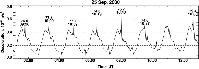
FIGURE 1. Accelerometer observations from the CHAMP satellite (Lühr et al., 2004) This plot shows 12 h of data, spanning a total of 8 orbits. The large-scale variations are the most obvious feature, with drag in the northern hemisphere being greater than in the southern hemisphere. This study, however, focuses on the narrow spikes that are associated with passes through the cusp region. The southern spikes are clearly much less significant than in the north. From Lühr et al. (2004).

Historically speaking, neutral upwelling was first observed in the very early days of space exploration, based on observations of satellite drag that was greater during times of enhanced solar activity (Jacchia, 1959). This was soon followed by a theory described by Jacchia and Slowey (1964), who attributed the effect to enhanced large-scale electric fields that drove Joule heating and the subsequent thermospheric heating.

The small-scale peaks in CHAMP data, however, are quite different than what was being addressed at that time, partly because the scale size of the peaks rendered them indetectable using the indirect measurements of decayed orbits that were used for that purpose. In fact, the small-scale peaks have since been linked to a number of distinct observables, including a high correlation with field-aligned currents (Kervalishvili and Lühr, 2013). Field-aligned currents imply the presence of electron precipitation that causes aurora, of course, and the soft electron precipitation associated with PMAFs has been highly correlated with ion upflow (Ogawa et al., 2003; Moen et al., 2004; Lynch et al., 2007). Not surprisingly, ion upflow has also been correlated with neutral upwelling as observed by CHAMP (Olson, 2012) and Kervalishvili and Lühr (2013), who reported a strong correlation between CHAMP thermospheric density anomalies with enhanced electron temperatures, small-scale field-aligned currents and ion up-flow in the cusp region.

To summarize, there appear to be two different processes that can drive neutral upwelling, one being large-scale Joule heating and the other being soft electron precipitation. These processes parallel two processes associated with ion upflow, as described by Wahlund et al. (1992). One process is associated with horizontal electric fields that drive convection and heat the ions without significant electron precipitation, which these authors call “Type 1” outflow (and this is the same basic process that was proposed by Jacchia and Slowey (1964) to cause thermospheric heating/upwelling).

The second mechanism is associated with aurora (i.e., electron precipitation) along with heated ionospheric electron populations, and is designated as “Type 2” outflow by Wahlund et al. (1992). It is this latter process that we consider in this paper that, as explained by Sadler et al. (2012), can also drive neutral upwelling. Essentially, these two mechanisms that drive ion upflow can also lift neutral particles via ion-neutral collisions (momentum transfer) with fast-moving ions transferring upward momentum to slow-moving neutrals.

1.1 The role of poleward moving auroral forms

Poleward Moving Auroral Forms (PMAFs) clearly play an important role in neutral upwelling, at least in the cases where the upwelling is due to auroral precipitation (i.e., Type 2 upflow). The prevalence of PMAFs in the cusp region is discussed by Fasel (1995), who examined 12 years of ground-based optical data from Longyearbyen, Svalbard. During that period, 476 days were examined, where the authors included only intervals occurring between 10:00–14:00 MLT (e.g., local magnetic noon). A total of 784 PMAF events were recorded over the course of the 58 days that had clear skies and aurora, suggesting that their occurrence is very common in the cusp.

As the name suggests, PMAFs consist of sets of auroral arcs that drift poleward, associated primarily with solar wind B_z < 0 conditions (Fasel, 1995) and controlled by the solar wind magnetic field as described by Sandholt et al. (2004), who note that the in Northern Hemisphere, PMAFs move westward when B_y is positive, and eastward when B_y is negative. Sandholt et al. (1990) describe PMAF dynamics, which are quite unique in terms of magnetosphere-ionosphere coupling. Figure 2 shows a typical PMAF event, one that occurred in conjunction with the Rocket Experiment for Neutral Upwelling 2 (RENU2) sounding rocket launch (Lessard et al., 2020). In this example, the early part of the keogram was acquired while there was snow on the optical dome, so the PMAF behavior is only clear beginning around 6:50 UT. The poleward motion of aurora, which typically includes numerous thin and dynamic arcs, is clear. The periodic repetition roughly every 10–15 min is also clear. This behavior is consistent with estimates provided by Sandholt et al. (1990), who determined that individual PMAFs have durations of 2–10 min and repeat roughly every 3–15 min.

FIGURE 2

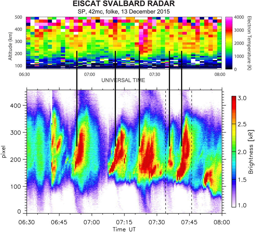
FIGURE 2. An elucidation of the PMAF effect. The lower panel shows a keogram of 630.0 nm emissions acquired at Longyearbyen of Poleward Moving Auroral Forms during the RENU2 launch. The upper panel shows electron temperature measurements acquired by the EISCAT radar, also at Longyearbyen. Electron temperature enhancements at altitudes from 200 to 400 km are observed as the various auroral forms drift into the EISCAT beam. The quasi-periodic occurrences of heated electron population (that establish ambipolar electric fields and subsequent ion upflow) are the basis for what we are calling the cusp “PMAF effect”.

An important consequence of PMAF activity has to do with the wide range of time scales involved in the coupling from soft electron precipitation to neutral upwelling. While a cold ionospheric electron population will be heated by these precipitating electrons within a small fraction of a minute and ion populations will be significantly heated over the course of several 10s of seconds, the much greater density (and heat capacity) of the neutral population requires 10 s of minutes to reach temperatures that will result in neutral upwelling (Sadler et al., 2012).

As the “first” PMAF passes over the cold ionosphere, it provides a source of precipitating electrons that is confined in latitude but that drifts over the entire region at ∼1 km/s for the event shown (analogous to waving a heat gun over an extended region). As it does so, the result of that activity is to transfer energy to a broad region in a transient manner with the end result depending on the state (i.e., the initial conditions) of the ionosphere and thermosphere. That is, because of the short time scales required for heating and cooling of electron and ion populations, these populations return to their nominal states fairly quickly. Heating and cooling of the neutral population, however, lags significantly behind, such that it does not cool to its initial state before a “second” PMAF enters the region, etc. Thus, each subsequent PMAF encounters different initial conditions that, in particular, include a progressively pre-heated neutral population. We denote this effect, where the shorter time scales of electron and ion dynamics transfer energy to thermosphere via quasi-periodic coupling of these populations, the “PMAF effect”.

In this paper, however, we do not model the complete PMAF effect (but see (Sadler et al., 2012), which does explain these details). We chose to focus on a PMAF-type of event because this is likely the most common scenario in the cusp during ion outflow and neutral upwelling, but the point here is to isolate interhemispheric differences. All that is discussed in this paper is what might be called an “initial”, individual PMAF effect.

1.2 The role of the ionosphere

As mentioned above, Sadler et al. (2012) show that soft electron precipitation can not only drive ion upflow, but that the upflowing ion population can then couple to the neutral particles and lift them to higher altitudes as well. Ion-neutral coupling in the model is incorporated using a momentum equation that calculates the change in momentum-density based on four terms including a) advection, b) pressure balance, c) ionization/recombination and d) momentum transfer. The model results imply, then, that interhemispheric differences in neutral upwelling may be associated with comparable differences in ion upflow and that the underlying cause of these interhemispheric differences perhaps lies in properties of the ionosphere, specifically its conductivity.

In fact, based on a statistical study of EISCAT data acquired between 1 March 2007 and 29 February 2008 (Ogawa et al., 2011), noted a strong seasonal dependence of ion upflow occurrence frequencies, specifically noting that the occurrence frequency of ion upflow events is ∼25% in winter, while only being ∼3% in the summer. On the other hand, upflowing fluxes are greater in the summer than in the winter.

A related study was carried out by Ji et al. (2019), who also used EISCAT data, but spanning the years 2000–2015. Their main objective was to determine occurrence frequencies of the various types of upflow, including not only Type 1 and Type 2, but also what they termed as Type 3 (Type 1 and 2) and Type 4 (neither Type 1 nor Type 2). While a main conclusion is that the highest frequencies occur with Type 3 (up to 40%), they also considered seasonal differences and note that maximum frequencies occur around winter solstice, with minimum frequencies during sumer solstice. in addition, they note lower occurrence frequencies during intervals of increases solar activity. All of these results imply that ionospheric conductivity plays an important role in ion upflow.

Other studies include that of Liu et al. (2001), who also used EISCAT data to observe upflow occurrences but focused on their connection to geomagnetic activity. They do also note, however, that the events show a “winter-over-summer” preference, consistent with the (Ogawa et al., 2011) and Ji et al. (2019). All three of these studies used EISCAT data with an event threshold of 100 m/s.

A possible explanation for this seasonal effect is provided by Cohen et al. (2015), who showed model results of ion upflow parameters having different initial electron density profiles during auroral precipitation events. These authors found that, in advance of the onset of soft precipitation, cases having increased electron density profiles led to smaller ionospheric (e.g., ambient) electron temperature increases and, therefore, weaker ambipolar fields. This is the field that is responsible for ion upflow and is consistent with our own model results.

The process works as follows. Precipitating electrons couple kinetic energy very efficiently to the cold background population (in the range of ∼250–400 km), driving significant increases in the temperature of that population and causing it to expand upwards and leading to a field-aligned electron pressure gradient. This pressure gradient is associated with an ambipolar electric field that can be described by the following equation (Cohen et al., 2015):

$E_a=\frac{-1}{e{n}_e}\nabla \left(k_B{n}_e{T}_e\right)=\frac{-k_B}{e}\left[\nabla T_e+T_e\frac{\nabla n_e}{n_e}\right](1)$

where E_a is the near-vertical ambipolar field, n_e is the electron density, T_e is the electron temperature, k_B is the Boltzmann constant and e is the elementary charge.

For a given precipitating electron input, the transfer of energy to a higher-density (e.g., sunlit) ionospheric electron population consequence is that, in a sunlit ionosphere, we should expect reduced upflow speeds but longer upflow timescales and larger upflow fluxes, consistent with the statistical studies discussed above. The implication is that reduced upflow speeds tend to lower the maximum speed below the 100 m/s event selection criteria that were used in Ogawa et al. (2011), Ji et al. (2019) and Liu et al. (2001), thereby leading to an apparent decrease in the occurrence rate. In order to illustrate the process quantitatively for each of the case studies presented below, we include estimates of electron temperatures as well as that of the ambipolar fields and ion upflow speeds associated with the soft electron precipitation.

2 Model description and results

The broad objective of this work is to characterize the physics of the coupling processes in order to lay the framework for further studies of PMAFs in a 2D geometry. As described above, any connection between PMAF activity and neutral upwelling in the cusp will need to account for overlapping timescales that range from a few seconds to tens of minutes. This is well within the capabilities of our model, though the model currently addresses dynamics only at a single location and uses a 1D field-aligned geometry (which is essentially vertical in the cusp region). Thus, it is not capable of modeling the integrated effects of a set of repetitive sequences of arcs passing over a specific extended region in the ionosphere/thermosphere (i.e., the full PMAF effect, in particular). On the other hand, in the context of exploring interhemispheric asymmetries, we are able to further advance our understanding of the role of the ionosphere and how it might impact cross-scale coupling.

The model implements a calculation of magnetosphere-ionosphere-thermosphere interactions from 100 km to 1,100 km with a gravitationally bound neutral MSIS-E-90 atmosphere of N₂, O₂ and O. The simulation uses a three-fluid model that includes inertial ion and neutral terms. It solves the continuity, momentum and energy equations for an average ion, neutral and electron component, with ionization, recombination and electron heating input based on an ionospheric transport model of Lummerzheim (1992). The electron energy equation incorporates ohmic heating and heating by precipitation, as well as conduction and advection and energy losses to neutrals. No mechanism is explicitly included to accelerate particles upward, although an ambipolar field develops as expected from the soft precipition. Basically, the model uses fundamental fluid model equations (continuity, momentum, energy, Ohms law) to produce a vertical electric (ambipolar) field, leading to “ambipolar diffusion.”

Inputs to the model include an ionospheric density profile, for which the International Reference Ionosphere (IRI) 2016 model was used with the appropriate date, time, and geographic location for each run. Altitude profiles were acquired from 100 km to 1,000 km with steps of 10 km. Output data included electron density, neutral temperature, electron temperature, O⁺ percentage, H⁺ percentage, He⁺ percentage, ${\mathrm{O}}_2^{+}$ percentage, NO⁺ percentage, and N⁺ percentage.

In order to understand interhemispheric differences in neutral upwelling and ion upflow, we concentrate on the variability of the ionosphere. However, since the IRI model only provides empirical estimates based on monthly averages, the variations in our study are primarily due to differences in solar elevation angles rather than ongoing magnetic activity. Our results illustrate the role of the ionosphere during these steady-state conditions in order to characterize the basic processes. They do not include changes in conductivity during a PMAF event as shown in Figure 2, for example.

Two steps were taken in this study. First, neutral upwelling was modeled for a single location in one hemisphere for four different ionospheric density profiles, including summer and winter solstices during solar maximum and solar minimum. This was done to keep the location (e.g., the magnetic coordinates) constant while varying only the density profiles. The location of Longyearbyen in Svalbard (78.2° Lat, 15.6° Lon, geographic) was used because this location routinely passes through the cusp (where ion upflow is most common).

The second step compares simultaneous, interhemispheric effects at Longyearbyen and at Zhongshan Station in Antarctica (−70.5° Lat, 76.2° Lon, geographic), roughly magnetic conjugate to Longyearbyen, with Longyearbyen in darkness and Zhongshan in sunlight.

2.1 Differences between a dark and sunlit ionosphere at a cusp location during solar minimum

Figure 3 shows the four ionospheric density profiles that were used in the first part of our study, all produced by the IRI model for Longyearbyen. For simply comparing the differences between a sunlit versus dark ionosphere at a cusp location, the IRI model was run for 21 December 2019 and 21 June 2019 (solar minimum) and for 21 June 2014 and 21 December 2013 (solar maximum). In all cases, the model was run using 09:30 UT, when Longyearbyen is approximately at magnetic noon. For the solar minimum case, the light blue trace shows the profile for a dark (e.g. winter) ionosphere and the yellow trace shows it for a sunlit (summer) ionosphere. For solar maximum, the dark blue trace is used for a dark ionosphere and the orange trace shows the profile for a sunlit ionosphere.

FIGURE 3

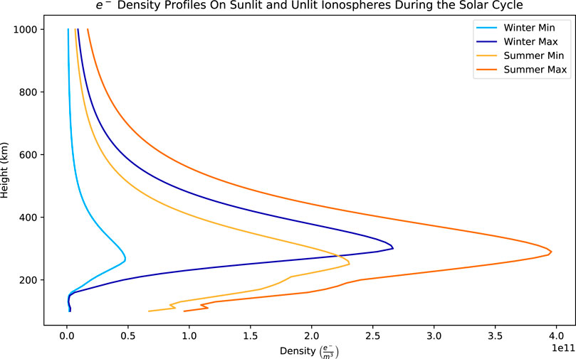
FIGURE 3. IRI density profiles for Longyearbyen for 4 different cases, to show the expected variability at that location (i.e., in the northern cusp). The light blue trace shows the profile for a dark (e.g. winter) ionosphere (21 Dec 2019) during solar minimum; the dark blue trace also shows the profile for a dark ionosphere, but during solar maximum (21 Dec 2013). The yellow trace shows the density for a sunlit (summer) ionosphere (21 Jun 2014) during solar minimum; the orange trace also shows the profile for a sunlit ionosphere, but during solar maximum (21 Jun 2014). All profiles were based on a time of 09:30 UT, which places Longyearbyen near the cusp region.

For each of these profiles, we ran the upwelling model by introducing soft electron precipitation having a Maxwellian distribution with a characteristic energy of 100 eV and an energy flux of 4 mW/m², as is commonly observed during cusp PMAFs. Figure 4 shows the results for solar minimum, with time (in minutes) along the horizontal axis. For altitudes of 400, 600 and 800 km, we show model predictions of ion upflow velocities, neutral particle velocities and relative neutral density variability. The top three panels show quantities during a sunlit ionosphere at Longyearbyen. The bottom three panels show these quantities during a dark ionosphere, at the same location.

FIGURE 4

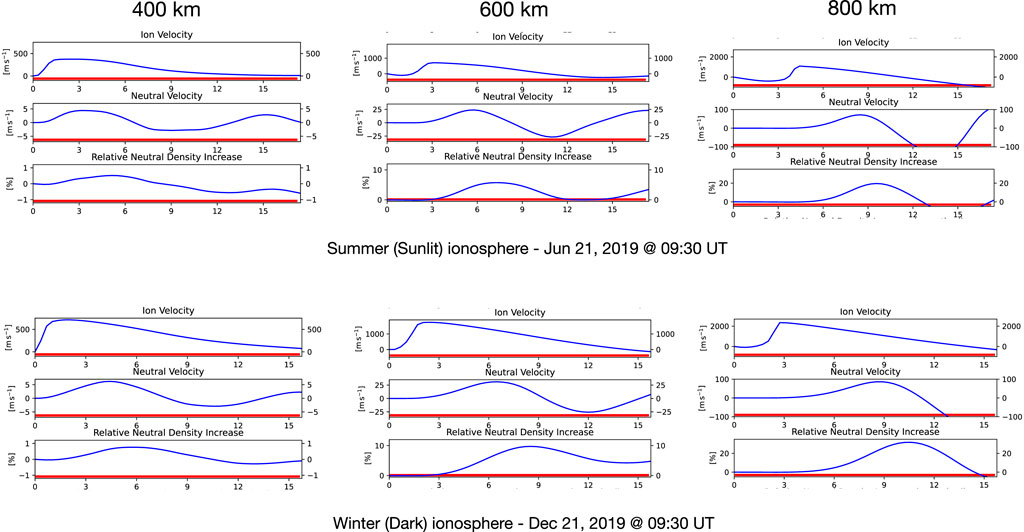
FIGURE 4. Model predictions of ion flow velocities, neutral particle velocities and relative neutral density variability during solar minimum. The top three panels show quantities during a sunlit ionosphere at Longyearbyean (typical cusp location), at altitudes of 400, 600 and 800 km. The bottom three panels show these quantities during a dark ionosphere, at the same location.

In order to interpret these results correctly, we remind the reader that this is a 1D model that can illustrate the upwelling process but it does not replicate the full PMAF effect. In this 1D case, electron precipitation will generate an ambipolar field that lifts the ions (and neutrals) upwards, leaving a depleted region behind as the event persists for several minutes. In a 2D case, the drifting arc will be continuously encountering an unperturbed ionosphere that would result in an extended region of ion upflow and neutral upwelling. This process can still leave a depleted region at lower altitudes, as shown in the plots and consistent with reports of depleted regions in upwelling events (Clemmons et al., 2008; Kervalishvili and Lühr, 2018; Lessard et al., 2020).

Interpretation of the results in Figure 4 is best accomplished by noting the various features that propagate to higher altitudes over time. Ion upflow speeds in sunlight are increased after ∼2 min at 400 km, reaching 375 m/s and, eventually, reaching 1,093 m/s at 800 km.

A neutral velocity enhancement occurs at 400 km, ∼3 min after the start of the run. It then appears at 600 km after about 5 min (at ∼14 m/s) and then at 800 km after ∼8 min with a speed of ∼71 m/s. There is also a second wave starting around 16 min at 400 km and as it propagates upward, the higher altitude plots show the tail end of the bump as the model time ends.

Regarding a density enhancement, we see an initial depletion at 400 km as the ion upflow begins and presumably drags the neutrals upwards, leaving the depletion. A density increase of ∼5.7% is seen at 600 km after 7–8 min and then a 19.6% increase at 800 km after ∼10 min. Comparing all quantities to the 600 and 800 km winter (dark) ionospheres, we see that ion upflow speeds, neutral velocity and density enhancements (up to ∼31.7% at 800 km) are all greater in a dark ionosphere. This is consistent with Cohen et al. (2015) results.

In terms of the physics behind the process that controls how a sunlit ionosphere modifies ion upflow speeds, we note the following results from the model. Once precipitation is turned on, ionospheric electron heating develops in a matter of seconds; the model shows that, after a period of 20 s, T_e will have increased to peak near ∼5234 K for a dark ionosphere but only ∼3568 K for a sunlit ionosphere. The elevated T_e causes the electron population to rapidly expand upwards and establishes an ambipolar field of 5.4 × 10⁻⁶ V/m in a dark ionosphere, while the cooler sunlit ionosphere leads to an ambipolar field of only 3.2 × 10⁻⁶ V/m. Again, Figure 4 shows that the upflow speeds vary accordingly, reaching ∼1750 m/s (at 600 km altitude) and ∼2,340 m/s (at 800 km) in darkness, compared to ∼708 m/s (at 600 km) and ∼1,093 m/s (at 800 km) in sunlight.

To summarize, the differences between upflow in a dark versus sunlit ionosphere (for solar minimum) are presented in Table 1. The values listed are the peak values during the model run, rather than an average. We take this approach because the peak values reflect the magnitude of the intensifications of these quantities and it is these structures that contribute to the upwelling observed by CHAMP.

TABLE 1

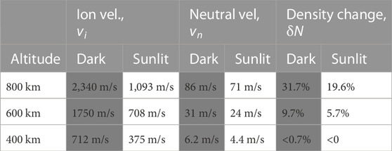
TABLE 1. Peak values for LYR during solar minimum, using a dark versus sunlit ionosphere. Boxes shaded in grey show values for a dark ionosphere.

2.2 Differences between a dark and sunlit ionosphere at a cusp location during solar maximum

Figure 5 uses the same format as Figure 4, but in the context of solar maximum. The expectation, of course, is that the increased conductivity due to the storm (see Figure 3) will tend reduce upflow speeds relative to solar minimum. Maximum values of the data shown in Figure 5 are summarized in Table 2.

FIGURE 5

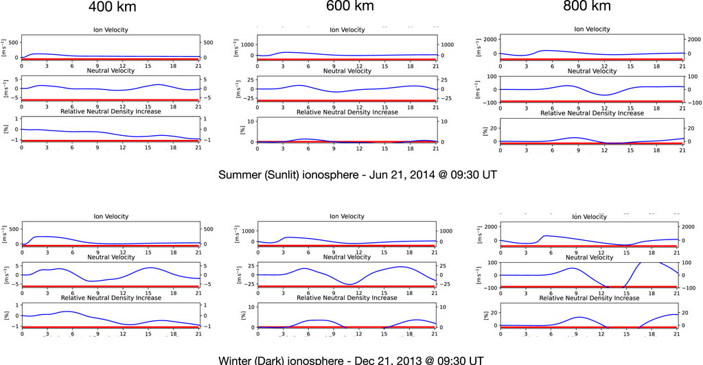
FIGURE 5. Model predictions of ion flow velocities, neutral particle velocities and relative neutral density variability during solar maximum. The top three panels show quantities during a sunlit ionosphere at Longyearbyean (typical cusp location), at altitiudes of 400, 600 and 800 km. The bottom three panels show these quantities during a dark ionosphere, at the same location.

TABLE 2

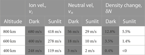
TABLE 2. Peak values for LYR during solar maximum, using a dark versus sunlit ionosphere. Boxes shaded in grey show values for a dark ionosphere.

In the upper panels of Figure 5, which shows results for a sunlit ionosphere, we see ion upflow speeds of 119 m/s at 400 km, increasing to 418 m/s at 800 km. The neutral population follows the same trend, as expected. Neutral upwelling occurs ∼2 min after the start of the run with an upflow speed of ∼2 m/s. The enhancement then appears at 600 km after about 5 min (at only ∼10 m/s) and then at 800 km after ∼8 min with a speed of only ∼29 m/s. There is also a second wave starting around 17 min at 400 km and as it propagates upward, the 600 km panel shows it at 19 min at ∼8 m/s.

Regarding the density enhancement in sunlight, we again see an initial depletion at 400 km as the ion upflow begins and presumably drags the neutrals upwards. A density increase of ∼1.4% is seen at 600 km after 6 min, leading to a 5.5% increase at 800 km after ∼9 min.

Comparing dynamics for this solar-maximum case to those of solar minimum, once precipitation is turned on and after a period of 20 s, T_e will have increased to peak near ∼3436 K for a dark ionosphere but only ∼2941 K for a sunlit ionosphere. The elevated T_e causes the electron population to rapidly expand upwards and establishes an ambipolar field of 2.6 × 10⁻⁶ V/m in a dark ionosphere, while the cooler sunlit ionosphere leads to an ambipolar field of only 2.2 × 10⁻⁶ V/m. Figure 5 shows that the upflow speeds vary accordingly, reaching ∼400 m/s (at 600 km altitude) and ∼680 m/s (at 800 km) in darkness, compared to ∼278 m/s (at 600 km) and ∼418 m/s (at 800 km) in sunlight.

The maximum values of density enhancements shown in the table are roughly half of what we see during solar minimum, presumably due to the lower upflow speeds. This seems counter-intuitive and, in fact, it is well known that ion outflow during storm times is dramatically increased, relative to non-stormtime events. The reason that the model leads to this result, we expect, is that the slower upward speeds simply require more time to develop the enhancement. Also, the lagging response of the neutral population may mean that the process fundamentally requires repeated PMAF passages, not just the isolated event described by the model.

2.3 Differences between a dark and sunlit ionosphere in opposite hemispheres

In this section, we present a specific case of interhemispheric ion upflow and neutral upwelling. We again include Longyearbyen as the northern hemispheric site, but add Zhongshan Station in Antarctica (−70.5° Lat and 76.2° Lon, geographic). Zhongshan Station is roughly magnetically conjugate to Longyearbyen, with Longyearbyen in darkness and Zhongshan in sunlight in this case. The date and time chosen coincide with the launch of the Rocket Experiment for Neutral Upwelling 2 (RENU2, Lessard et al. (2020)), 13 December 2015 at 07:34 UT. We use this date because EISCAT Svalbard and other data readily available, including the measured ionospheric density profile at Longyearbyen.

Figure 6 shows Ionospheric density profiles for this event. The blue trace shows IRI predictions for Longyearbyen. The green trace shows EISCAT measurements at 7:34 UT, “in between” PMAF auroral arcs. Again, the IRI model produces an average density profile and would not be expected to show the quasi-periodic nature of PMAF activity. The EISCAT data are quite similar to the IRI model results, except that the profile appears at a lower altitude. The orange trace shows IRI predictions for Zhongshan Station in Antarctica, with the extended F-region peak showing the effects of sunlight at that location.

FIGURE 6

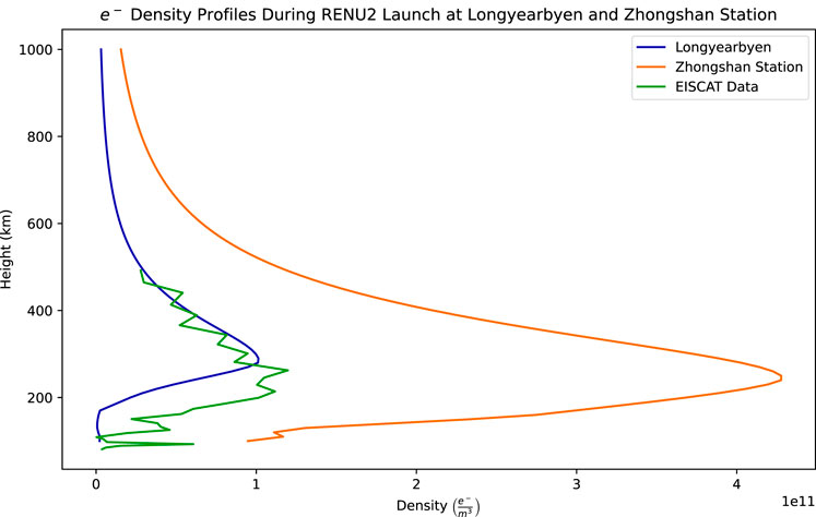
FIGURE 6. Ionospheric density profiles during the RENU2 launch. The blue trace shows IRI predictions; the green trace shows EISCAT observations at 7:34 UT, “in between” auroral arcs, which is similar to the IRI results except at a somewhat lower altitude. The orange trace shows IRI predictions for Zhongshan Station in Antarctica, nominally conjugate to Longyearbyen.

Figure 7 shows model predictions of upflow velocities, neutral particle velocities and relative neutral density variability, with the same format as in the previous figures. The upper panels show results for Zhongshan Station while it is sunlit, the bottom panel shows results for Longyearbyen, in darkness.

FIGURE 7

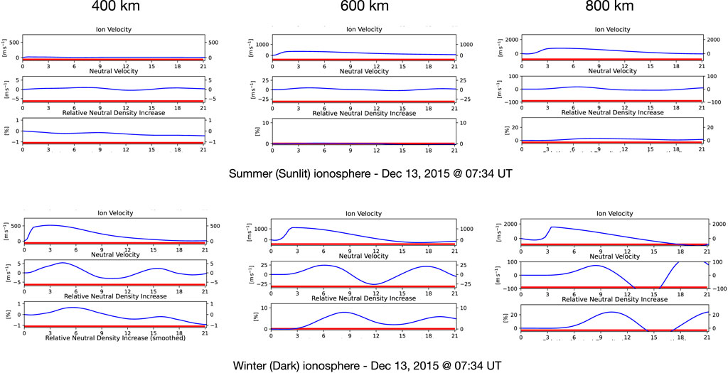
FIGURE 7. Model predictions of ion flow velocities, neutral particle velocities and relative neutral density variability, with the same format as in the previous figures. This provides an example of simultaneous interhemispheric predictions, with Zhongshan Station (Antarctica) in the southern hemisphere being in sunlight and Longyearbyen in the northern hemisphere, darkness. Density profiles for these model runs are shown in Figure 6.

Table 3 summarizes the important values from Figure 7. In the upper panel of that figure, we see ion upflow speeds for a sunlit ionosphere reaching 362 m/s at 600 km and increasing to 762 m/s at 800 km. Again, the neutral upwelling speeds are only a fraction of the ion upflow speeds, being 5 m/s at 600 km and 17 m/s at 800 km. This upwelling leads to an increase in density of ∼0.6% at 600% and 3.0% at 800. As seen in the lower panel, showing LYR in darkness, the model predicts ion upflow speeds of 1,110 m/s at 600 km and 1,580 m/s at 800 km. The neutral upwelling speeds are only 17 m/s and 73 m/s at these altitudes, while the density enhancements are 3.0% and 21.4%.

TABLE 3

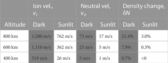
TABLE 3. Peak values for the simultaneous modeling of Longyeabyen (in darkness) and Zhongshan (in sunlight) for 13 December 2015 at 07:34 UT. Boxes shaded in grey show values for a dark ionosphere.

Interpretation of the process is similar to the case studies above. Once precipitation is turned on, after a period of 20 s, T_e will have increased to peak near ∼4254 K for a dark ionosphere but only ∼4348 K for a sunlit ionosphere, just slightly greater than for a dark ionosphere. The elevated T_e causes the electron population to rapidly expand upwards and establishes an ambipolar field of 3.8 × 10⁻⁶ V/m in a dark ionosphere, while the cooler sunlit ionosphere leads to an ambipolar field of only 2.6 × 10⁻⁶ V/m. Again, Figure 5 shows that the upflow speeds vary accordingly, reaching ∼1,110 m/s (at 600 km altitude) and ∼1,580 m/s (at 800 km) in darkness, compared to ∼362 m/s (at 600 km) and ∼762 m/s (at 800 km) in sunlight.

2.3.1 The role of the thermosphere

Cannata and Gombosi (1989) present results from a numerical study of solar cycle variations of the thermosphere and how these variations modify the composition and intensity of ion upflows during solar minimum and maximum. The authors attribute the effects to EUV/UV-driven thermospheric increases in atomic oxygen and, based on this consideration, show numerical ion upflow results comparable to in situ observations. Pham et al. (2021) also carried out a numerical study, with their results showing how thermospheric regulation of ion outflows can modify ionospheric convection in such a way as to provide feedback that modifies the evolving O⁺ outflow process. Consistent with Cannata and Gombosi (1989), these authors also highlight the fact that during active times (e.g., increased F10.7), the neutral atomic oxygen density is increased and photoionization of that population directly supports increased O⁺ outflow.

The results from our study show a related, but unexpected and important outcome. Tables 1 and 2 show ion and neutral upflow speeds during solar minimum and solar maximum, respectively. The case presented in Table 3 was chosen because it coincided with the RENU2 launch in December 2015, which occurred near solar maximum (Solar Cycle 24 reached its maximum in April 2014).

We consider momentum transfer from ions to neutrals in the case of a sunlit ionosphere, focusing on the ratios of neutral upflow speeds to ion upflow speeds, $v_{n_{\mathit{Sunlit}}}/v_{i_{\mathit{Sunlit}}}$. Focusing on effects at 800 km (results at 600 km are comparable), from Table 1 the ratio is 71/1,093 = 0.065, while from Table 2 it is 29/418 = 0.069. The ratio from Table 3, however is only 17/762 = 0.022, reduced from the other two cases by a factor of ∼3. That is, the relative neutral upflow speeds are lower in a sunlit thermosphere.

The reason for this difference lies in the fact that the thermospheric temperature and density for Zhongshan are both higher than in the other cases discussed above. Presumably driven by intense and persistent sunlight (24-h sunlight, with significant reflectivity from a very high albedo from the snow in Antarctica), the MSIS-E−90 model predicts the temperature to be 1235 K at 1,000 km, significantly higher than the 820 K (at 800 km) predicted for Longyearbyen. Our model incorporates this information via the inclusion of 3 “typical” neutral profiles that are built-in to the model and specified by the temperature at 1,000 km altitude as 883 K, 1044 K or 1304 K. For this particular case, the 1235 K prediction by MSIS-E−90 is accomodated using our model’s 1304 K version of the neutral atmosphere.

The physics behind this process involves ion upflow, of course. As with each of the cases in this study, the driver begins with soft electron precipitation, e.g., a Maxwellian distribution with a characteristic energy of 100 eV and an energy flux of 4 mW/m². With Zhongshan being in a sunlit ionosphere, the upflowing ion speeds will tend to be reduced (relative to a dark ionosphere) but would be expected to be comparable to the sunlit examples in Sections 2.1 and Section 2.2 above. As the ions drift upwards, momentum will be transferred to the neutral particles due to ion-neutral collisions. In the first 2 cases, this led to $v_{n_{\mathit{Sunlit}}}/v_{i_{\mathit{Sunlit}}}$ being the order of 6.7%. In the third case, however, the increased density in the thermosphere equates to a greater mass that needs to be accelerated upwards. The net result is that the upward velocity of the greater mass leads to a decreased upflowing particle speed, on average. The model predicts that $v_{n_{\mathit{Sunlit}}}/v_{i_{\mathit{Sunlit}}}$ is only $\sim 2$% in this case.

If momentum transfer is a key component of the process, then the ratio of neutral upflow speeds to ion upflow speeds presumably depends on the ratio of the neutral density to the ion density. Using results from the model runs, we find that the peak ratio of these densities are ${\rho }_{n_{\mathit{LYR}}}/{\rho }_{i_{\mathit{LYR}}}\sim$8 at 600 km and $<$1 at 800 km for Longyearbyen. On the other hand, the values are much greater for Zhongshan, being ${\rho }_{n_{\mathit{ZHO}}}/{\rho }_{i_{\mathit{ZHO}}}\sim$55 at 600 km and 15 at 800 km, consistent with the idea that a greater relative neutral density results in a decreased neutral upward velocity.

Finally, It is important to note that the concept of ion-neutral coupling via momentum exchange, including how a denser thermosphere leads to lower upflow speeds, is valid where the ion upflow is driven by electron precipitation (Type 2) or by Joule heating (Type 1).

3 Discussion

We studied three scenarios to highlight how ionospheric conductivity might be responsible for modifying or controlling the rates and/or speeds of ion upflow and neutral upwelling. Each case used Longyearbyen, Svalbard as a key location because of its high magnetic latitude that generally has it routinely passing through the noon-time cusp, a feature that has historically made that location very important for upflow studies. We also take advantage of the fact that Longyearbyen is approximately magnetically conjugate to Zhongshan Station in Antarctica. Results are summarized in the tables above.

Our study does not include effects of Joule heating because the goal has been to isolate/study PMAF effects. However, Ji et al. (2019) determined that up to 40% of EISCAT upflow events coincided with a combination of Type 1 (Joule heating) and Type 2 (electron precipitation) drivers. It may be for this reason that the density enhancements predicted by our model are somewhat less than what is observed by CHAMP.

Relating the model results presented here to the CHAMP observations is problematic in this simple study. Unlike CHAMP measurements that show an integregated effect over a 2D region (altitude versus the satellite trajectory), our model considers only the 1D case. Visualizing a 2D version of our result by simply replacing changes in time with changes in space would not be appropriate because of the PMAF effects described above. Such a strategy would produce a uniform extended region with a density enhancement of the magnitude that the 1D model predicts with the passage of the first PMAF.

As described above, the first PMAF in a sequence might encounter a quiet ionosphere as it drifts poleward. The time scales required for the thermosphere to respond to various inputs is several tens of minutes, while the intervals between PMAF passages is the order of 10–15 min. This means that the ionosphere/thermosphere system does not have time to relax to its original state before the next PMAF arrives, i.e., that subsequent PMAFs will encounter different “initial conditions”. While a 1D model cannot track these dynamics, this study does provide the opportunity to investigate the basic effects that ionospheric conductivity has on this process.

Our study leads to the following conclusions.

1. Although our model considers only 1D, we show that ionospheric density profiles play a fundamentally important role in ion upflow and neutral upwelling. For each of the 3 scenarios, we show that ion upflow speeds, neutral upwelling speeds and neutral density enhancements are all significantly greater in a dark ionosphere, by perhaps as much as a factor or 2 or 3, relative to a sunlit ionosphere.

2. Noting that neutral upwelling speeds are less than ion upflow speeds in all cases, our results suggest (also see Sadler et al., 2012) that upflowing ions are the driver of neutral upwelling via ion-neutral collisions (momentum transfer), with fast-moving ions transferring upward momentum to slow-moving neutrals. This implies that the speeds of neutral upwelling particles must also be greater in a dark ionosphere, which is what the model results show in all cases.

3. From the various case studies, we note an interesting and unexpected result by considering the ion and neutral relative velocities. Specifically, from Table 1, the ratio $v_{n_{\mathit{Sunlit}}}/v_{i_{\mathit{Sunlit}}}$ at 800 km (results at 600 km are comparable) is 71/1,093 = 0.065, while from Table 2 it is 29/418 = 0.069. The ratio from Table 3, however is only 17/762 = 0.022, reduced from the other two cases by a factor of ∼3. The model results imply that this is due to a greater neutral density at Zhongshan, where the effect for a given input is that the increased density leads to an average decreased velocity (per particle) of the upwelling population.

Data availability statement

The raw data supporting the conclusion of this article will be made available by the authors, without undue reservation.

Author contributions

The general concept for this study was provided by ML, who also wrote the bulk of the text for this paper. FS implemented numerous improvements in the neutral upwelling model and provided guidance for its use. AD acquired appropriate ionospheric profiles and used this input to carry out the detailed modeling work. KO provided the EISCAT data and comments. LC processed the allsky camera data and provided the auroral keogram. All authors contributed to the article and approved the submitted version.

Funding

This work was supported at the University of New Hampshire by NASA Grants 80NSSC21K0972 and NNX17A138G. KO is supported by the Research Council of Norway Grant 223252. ML thanks the International Space Science Institute in Bern for their support of the ISSI team “Understanding Interhemispheric Asymmetry in MIT Coupling,” which enabled excellent discussions on this topic.

Acknowledgments

The authors would like to thank the undergraduate and graduate student researchers, faculty, and staff of the Magnetosphere-Ionosphere Research Laboratory at the University of New Hampshire for their input and scientific expertise. The authors also thank the EISCAT Svalbard radar facility for providing the ground-based data. EISCAT is an international association supported by research organizations in China (CRIRP), Finland (SA), Japan (NIPR and STEL), Norway (NFR), Sweden (VR), and the United Kingdom (NERC). EISCAT data were from the Madrigal Database at EISCAT, https://madrigal.eiscat.se/madrigal.

Conflict of interest

The authors declare that the research was conducted in the absence of any commercial or financial relationships that could be construed as a potential conflict of interest.

Publisher’s note

All claims expressed in this article are solely those of the authors and do not necessarily represent those of their affiliated organizations, or those of the publisher, the editors and the reviewers. Any product that may be evaluated in this article, or claim that may be made by its manufacturer, is not guaranteed or endorsed by the publisher.

References

Cannata, R. W., and Gombosi, T. I. (1989). Modeling the solar cycle dependence of quiet-time ion upwelling at high geomagnetic latitudes. Geophys. Res. Lett. 16, 1141–1144. doi:10.1029/GL016i010p01141

CrossRef Full Text | Google Scholar

Clemmons, J. H., Hecht, J. H., Salem, D. R., and Strickland, D. J. (2008). Thermospheric density in the Earth’s magnetic cusp as observed by the Streak mission. Geophys. Res. Lett. 35, 24103. doi:10.1029/2008GL035972

CrossRef Full Text | Google Scholar

Cohen, I. J., Lessard, M. R., Varney, R. H., Oksavik, K., Zettergren, M., and Lynch, K. A. (2015). Ion upflow dependence on ionospheric density and solar photoionization. J. Geophys. Res. Space Phys. 120, 10039–10052. doi:10.1002/2015ja021523

CrossRef Full Text | Google Scholar

Fasel, G. J. (1995). Dayside poleward moving auroral forms: a statistical study. J. Geophys. Res. 100, 11891. doi:10.1029/95JA00854

CrossRef Full Text | Google Scholar

Jacchia, L. G. (1959). Corpuscular radiation and the acceleration of artificial satellites. Nature 183, 1662–1663. doi:10.1038/1831662a0

CrossRef Full Text | Google Scholar

Jacchia, L. G., and Slowey, J. (1964). Atmospheric heating in the auroral zones: a preliminary analysis of the atmospheric drag of the injun 3 satellite. J. Geophys. Res. 69, 905–910. doi:10.1029/jz069i005p00905

CrossRef Full Text | Google Scholar

Ji, E.-Y., Jee, G., and Lee, C. (2019). Characteristics of the occurrence of ion upflow in association with ion/electron heating in the polar ionosphere. J. Geophys. Res. Space Phys. 124, 6226–6236. doi:10.1029/2019JA026799

CrossRef Full Text | Google Scholar

Kervalishvili, G. N., and Lühr, H. (2018). “Climatology of air upwelling and vertical plasma flow in the terrestrial cusp region: seasonal and IMF-dependent processes,” in Of astrophysics and space science library. Magnetic fields in the solar system. Editors H. Lühr, J. Wicht, S. A. Gilder, and M. Holschneider, 448, 293–329. doi:10.1007/978-3-319-64292-5_11

CrossRef Full Text | Google Scholar

Kervalishvili, G. N., and Lühr, H. (2013). The relationship of thermospheric density anomaly with electron temperature, small-scale FAC, and ion up-flow in the cusp region, as observed by CHAMP and DMSP satellites. Ann. Geophys. 31, 541–554. doi:10.5194/angeo-31-541-2013

CrossRef Full Text | Google Scholar

Lessard, M. R., Fritz, B., Sadler, B., Cohen, I., Kenward, D., Godbole, N., et al. (2020). Overview of the rocket experiment for neutral upwelling sounding rocket 2 (RENU2). Geophys. Res. Lett. 47, e81885. doi:10.1029/2018GL081885

CrossRef Full Text | Google Scholar

Liu, H., Ma, S.-Y., and Schlegel, K. (2001). Diurnal, seasonal, and geomagnetic variations of large field-aligned ion upflows in the high-latitude ionospheric f region. J. Geophys. Res. Space Phys. 106, 24651–24661. doi:10.1029/2001JA900047

CrossRef Full Text | Google Scholar

Lühr, H., Rother, M., Köhler, W., Ritter, P., and Grunwaldt, L. (2004). Thermospheric up-welling in the cusp region: evidence from CHAMP observations. Geophys. Res. Lett. 31, L06805. doi:10.1029/2003GL019314

CrossRef Full Text | Google Scholar

Lummerzheim, D. (1992). Comparison of energy dissipation functions for high energy auroral electron and ion precipitation. Fairbanks: Geophys. Inst. Univ. of Alaska. Rep. uag-r-318.

Google Scholar

Lynch, K. A., Semeter, J. L., Zettergren, M., Kintner, P., Arnoldy, R., Klatt, E., et al. (2007). Auroral ion outflow: low altitude energization. Ann. Geophys. 25, 1967–1977. doi:10.5194/angeo-25-1967-2007

CrossRef Full Text | Google Scholar

Moen, J., Oksavik, K., and Carlson, H. C. (2004). On the relationship between ion upflow events and cusp auroral transients. Geophys. Res. Lett. 31, L11808. doi:10.1029/2004GL020129

CrossRef Full Text | Google Scholar

Ogawa, Y., Buchert, S. C., Häggström, I., Rietveld, M. T., Fujii, R., Nozawa, S., et al. (2011). On the statistical relation between ion upflow and naturally enhanced ion-acoustic lines observed with the EISCAT Svalbard radar. J. Geophys. Res. Space Phys. 116, A03313. doi:10.1029/2010JA015827

CrossRef Full Text | Google Scholar

Ogawa, Y., Fujii, R., Buchert, S. C., Nozawa, S., and Ohtani, S. (2003). Simultaneous EISCAT Svalbard radar and DMSP observations of ion upflow in the dayside polar ionosphere. J. Geophys. Res. (Space Phys. 108, 1101. doi:10.1029/2002JA009590

CrossRef Full Text | Google Scholar

Olson, D. K. (2012). Neutral Gas and plasma Interactions in the polar Cusp. phd thesis. Maryland: University of Maryland.

Google Scholar

Pham, K. H., Lotko, W., Varney, R. H., Zhang, B., and Liu, J. (2021). Thermospheric impact on the magnetosphere through ionospheric outflow. J. Geophys. Res. Space Phys. 126. doi:10.1029/2020JA028656

CrossRef Full Text | Google Scholar

Rentz, S., and Lühr, H. (2008). Climatology of the cusp-related thermospheric mass density anomaly, as derived from CHAMP observations. Ann. Geophys. 26, 2807–2823. doi:10.5194/angeo-26-2807-2008

CrossRef Full Text | Google Scholar

Sadler, F. B., Lessard, M., Lund, E., Otto, A., and Lühr, H. (2012). Auroral precipitation/ion upwelling as a driver of neutral density enhancement in the cusp. J. Atmos. Solar-Terrestrial Phys. 87, 82–90. doi:10.1016/j.jastp.2012.03.003

CrossRef Full Text | Google Scholar

Sandholt, P. E., Farrugia, C. J., and Denig, W. F. (2004). Dayside aurora and the role of imf |B_y|/|B_z| detailed morphology and response to magnetopause reconnection. Ann. Geophys. 22, 613–628. doi:10.5194/angeo-22-613-2004

CrossRef Full Text | Google Scholar

Sandholt, P. E., Lockwood, M., Oguti, T., Cowley, S. W. H., Freeman, K. S. C., Lybekk, B., et al. (1990). Midday auroral breakup events and related energy and momentum transfer from the magnetosheath. J. Geophys. Res. Space Phys. 95, 1039–1060. doi:10.1029/JA095iA02p01039

CrossRef Full Text | Google Scholar

Wahlund, J.-E., Opgenoorth, H. J., Haggstrom, I., Winser, K. J., and Jones, G. O. L. (1992). EISCAT observations of topside ionospheric ion outflows during auroral activity - revisited. J. Geophys. Res. 97, 3019–3037. doi:10.1029/91ja02438

CrossRef Full Text | Google Scholar