 Astrid Maute
 Jeffrey M. Forbes
 Chihoko Y. Cullens3
95% of researchers rate our articles as excellent or good
Learn more about the work of our research integrity team to safeguard the quality of each article we publish.
Find out more
ORIGINAL RESEARCH article
Front. Astron. Space Sci. , 22 March 2023
Sec. Space Physics
Volume 10 - 2023 | https://doi.org/10.3389/fspas.2023.1147571
This article is part of the Research Topic Vertical Coupling in the Atmosphere-Ionosphere-Magnetosphere System View all 21 articles
Introduction: The vertical coupling of the lower and upper atmosphere via atmospheric solar tides is very variable and affects the thermosphere and ionosphere system. In this study, we use Ionospheric Connection (ICON) explorer data from 220–270 Day Of Year (DOY), 2020 when large changes in the migrating semidiurnal tide (SW2) and the zonal and diurnal mean (ZM) zonal wind occur within 8 days.
Method: We use the ICON Level4 product, the thermosphere-ionosphere-electrodynamics general circulation model (TIEGCM) driven by tides fitted to ICON observations via the Hough Mode Extension (HME) method. The effect of the upward propagating tides is isolated by examining the difference between two TIEGCM simulations with and without tidal HME forcing at the model lower boundary.
Results: The simulations reveals that the solar SW2 changes its latitudinal structure at 250 after DOY 232 from two peaks at mid latitudes to one broad low latitude peak, while at 110 km the two-peak structure persists. The ZM zonal wind at 250 km undergoes a similar dramatic change. These SW2 changes are associated with the prevalence of antisymmetric HMEs after DOY 232. The migrating diurnal, terdiurnal and quaddiurnal tides at 250 km undergo similar variations as SW2. TW3 is strong in the thermosphere and most likely caused by non-linear tidal interaction between DW1 and SW2 above 130 km. Surprisingly, the solar in situ forcing of TW3 and SW2 in the upper thermosphere is not nearly as important as their upward propagating tidal component. Associated with the strong dynamical changes, the zonal and diurnal mean NmF2 decreases by approximately 15%–20%, which has a major contribution from the O/N2 decrease by roughly 10%. These changes are stronger than general seasonal behavior.
Discussion: While studies have reported on the dynamical changes via SW2 in the mesosphere-lower thermosphere (MLT) region during the equinox transition period, this study is, to our knowledge, the first to examine the effects of rapid changes in SW2 on the upper thermosphere and ionosphere. The study highlights the potential of using ICON-TIEGCM for scientific studies.
Solar atmospheric tides excited in the lower atmosphere can propagate into the lower thermosphere where they modify among others, the neutral wind circulation, the composition, and the electrodynamics. Some tides can even propagate into the upper thermosphere, directly changing the plasma distribution. The Ionosphere Connection (ICON) explorer (Immel et al., 2018) is designed to study the connection between the lower and upper atmosphere by observing key quantities. The value of the ICON observations are demonstrated in many studies (e.g., Immel et al., 2021; Cullens et al., 2022; England et al., 2022; Harding et al., 2022; Heelis et al., 2022). The ICON mission is augmented by accompanying numerical simulations to enhance the scientific return (e.g., Forbes et al., 2017; Huba et al., 2017; Maute, 2017; Cullens et al., 2020). In this study, we demonstrate the value of these simulations in aiding the interpretation of the ICON observations during the August-September 2020 time period.
Upward propagating solar tides from the lower atmosphere have a rich spectrum due to different generation processes, i. e., absorption of solar radiation by tropospheric water vapor, by stratospheric ozone, by lower thermospheric molecular oxygen, by thermospheric atomic oxygen, and latent heat release in the tropics due to deep convection (e.g., Butler and Small, 1963; Lindzen and Chapman, 1969; Forbes, 1982b; a; Hagan et al., 2007). In addition, depending on tidal characteristics and the mean atmospheric conditions, tides might propagate upward, are modulated, dissipate, and/or interact non-linearly with other tides, planetary waves, and gravity waves (e.g., Holton, 1975; Volland, 1988; Miyahara and Forbes, 1991). In the following, we use the term “upward propagating lower atmospheric tides” for the tidal spectrum close to 97 km.
In this study, our primary focus is on the various harmonics of solar tides with frequencies nΩ and zonal wavenumbers s = n, denoted [n, s], where Ω = 2π/24 h. Here, if n and s are equal and s is positive it implies westward migration with the apparent motion of the Sun to a ground-based observer, and thus are referred to as “migrating” tides. We use the common shorthand notation DW1, SW2, TW3 and QW4 to denote migrating diurnal (D), semidiurnal (S), terdiurnal (T) and quaddiurnal (Q) tides, respectively. We use alternatively [1, 1], [2, 2], [3, 3], and [4, 4] when quantifying primary and secondary waves engaged in non-linear interactions. Stationary planetary waves are denoted by SPWs or [0, s] and the zonal and diurnal mean as ZM = [0, 0]. Eastward propagating tides are denoted by an “E” e.g., SE2 is the eastward propagating semidiurnal tide with zonal wavenumber 2 or [2,-2].
It is now well accepted, based on both, observations and theory, that the interaction between two primary waves [n1, s1] and [n2, s2] results in two secondary waves (sw) with frequencies and zonal wavenumbers that are the sums and differences of the frequencies and zonal wavenumbers of the primary waves: sw+ = [n1+n2, s1+s2], sw- = [n1-n2, s1-s2] (e.g., see Teitelbaum and Vial, 1991). These relationships will be used in the current study to identify the likely origins of some waves.
The current study focuses on the time period August 7 - 26 September 2020 (Day of Year DOY 220–270) when the migrating semidiurnal tide (SW2) and the thermospheric background circulation exhibits large, sudden changes. This period is close to the equinox transition time, therefore we will provide some overview of associated studies in the following, even though in the discussion of our results we do not focus on a connection to the equinox transition.
The equinox transitions in thermosphere and ionosphere (TI) are complex since the TI is influence by processes in different regions, each with their associated seasonal behavior, e.g., lower atmospheric upward propagating tides (e.g., Hagan and Forbes, 2002, 2003; Oberheide et al., 2011a) and corresponding changes in the mean circulation and composition (e.g., Fesen et al., 1991; Fuller-Rowell, 1998), in situ processes such as direct solar radiation (e.g., Ward et al., 2021), and coupling to the polar regions (e.g., Millward et al., 1996). Therefore, studies have shown that the equinox transition exhibits variability from year to year and does not necessarily align with the solar equinox (e.g., Pancheva et al., 2009; Burns et al., 2012; Venkateswara Rao et al., 2015).
While seasonal changes occur all the time, recently Conte et al. (2018) reported on a sharp semidiurnal solar tidal (S2) amplitude decrease during the equinox transitions, especially around September, which was observed by three meteor radars in the northern hemisphere and southern hemisphere (Conte et al., 2017). They found that the S2 decrease extends from the mesosphere to the lower thermosphere (approximately 75–100 km) with varying onset DOY (between DOY 265–295) for different years. By employing the Hamburg Model of the Neutral and Ionized Atmosphere (HAMMONIA) model (Schmidt et al., 2006), the authors could attribute the S2 changes mainly to distinct SW2 tidal changes with some contribution from SW1 later in the seasonal transition.
In a follow on study, Pedatella et al. (2021) used the Specified Dynamics Whole Atmosphere Community Climate Model with thermosphere-ionosphere eXtension simulations (SD-WACCMX) to find that during the September transition the antisymmetric Hough modes (2,3) and (2,5) are decreasing in amplitude leading to the decrease in SW2 amplitude. The timing of the lower thermospheric SW2 transition was linked to the seasonal transition in the middle atmosphere. Other studies have also used differences in Hough modes and vertical wavelengths to understand the changes in the SW2 latitudinal variation with altitude (e.g., Azeem et al., 2016; Stober et al., 2021; Forbes and Zhang, 2022). In addition, signals of distinct September transitions are observed in the D-region ionosphere in the propagation of very low frequency (VLF) radio wave signals (Macotela et al., 2021), suggesting an association with the mean temperature variation at 70–80 km and the semidiurnal solar tidal enhancement.
As noted by Pedatella et al. (2021), evolution of the latitude structure of SW2 during the 1–2 months leading up to solar equinox (DOY 266) is complex, and characterized by asymmetries between hemispheres that vary from year to year. While the troposphere and stratosphere excitations of SW2 project mainly onto the first symmetric mode of SW2 during both equinox and solstice conditions (e.g., Forbes and Garrett, 1978), it is the interaction of this mode with the middle atmosphere zonal wind field that plays a strong role in exciting antisymmetric modes through “mode coupling” (Lindzen and Hong, 1974) or “cross coupling” (Walterscheid and Venkateswaran, 1979a; b). Moreover, vertical propagation of the first symmetric mode of SW2 is sensitive to the vertical temperature gradient in the mesosphere (Geller, 1970; Forbes et al., 2022). At lower thermospheric heights, these modes, all with different vertical and latitudinal structures, achieve their largest amplitudes and constructively and destructively interfere as a function of time to produce the evolution of latitude structures at any given height that comprise the complexity noted above.
Several studies examined the connection between different migrating tidal changes in the mesosphere-lower thermosphere region (MLT) during the September-October season and we mention only a few recent ones in the following. van Caspel et al. (2020) used 16 years of northern hemisphere high latitude Super Dual Auroral Radar Network (SuperDARN) meteor winds finding the largest SW2 amplitudes in early fall of all seasons (peaking around DOY 260) and they attributed the seasonal variation of SW2 mainly to the changes in the background atmospheric conditions (e.g., Hagan et al., 1999). In addition, the authors reported on a pronounced migrating terdiurnal tidal (TW3) peak at DOY 265, which agrees with modeling results by Du and Ward (2010); Conde et al. (2018) reported on terdiurnal tides in meteor radar (40N–70N) with sudden changes starting after DOY 250.
Terdiurnal tides can be generated by the non-linear interaction between diurnal and semidiural tides (e.g., Teitelbaum et al., 1989; Smith, 2000; Younger et al., 2002) and/or diurnal tides with gravity waves (Miyahara and Forbes, 1991), and direct solar forcing. There is still discussion about the importance of these different mechanisms with season and we refer to the literature for more insights. Direct solar forcing was identified as the dominant TW3 driver during all seasons (e.g., Smith and Ortland, 2001; Du and Ward, 2010; Lilienthal et al., 2018). Non-linear interaction between tides and/or gravity waves were found to become more important in January and April (Lilienthal et al., 2018). Akmaev (2001) stated that non-linear interactions play a role especially at equinox between 95 and 100 km. Similarly, Huang et al. (2007); Moudden and Forbes (2013) determined that non-linear tidal interaction of DW1 and SW2 is important in TW3 excitation and is overlaid on the upward propagating part.
In general, the terdiurnal tides in the zonal and meridional wind is small in the MLT region, roughly around 4–6 m/s with peaks around equinox (e.g., Du and Ward, 2010; Liu et al., 2020; Pancheva et al., 2021). This could be a factor why less is known about the terdiurnal tide in the upper thermosphere. Gong and Zhou (2011) reported on the terdiurnal tide in the meridional wind between 90 and 350 km at Arecibo for January 2010, finding amplitude in the F-region smaller than the diurnal tidal amplitudes but larger than the semidiurnal tides. Note that the terdiurnal tide at a location is the superposition of various terdiurnal tides with different zonal wavenumbers and can therefore be an over- or underestimation of TW3 (e.g., Du and Ward, 2010).
The quaddiurnal tide is in general even smaller than the terdiurnal tide in the MLT region and therefore not the focus of many studies. Jacobi et al. (2017) examined meteor radar observations at mid-latitude in Europe, finding that the quaddiurnal tide in the zonal wind is up to 7 m/s around December and approximately 1–2 m/s in August-September with much shorter vertical wavelength in northern hemisphere summer than winter. Model diagnostics indicate that the non-linear tidal interactions contribute to the generation of the quaddiurnal tides (e.g., Smith et al., 2004). However, Geißler et al. (2020) found through numerical experiments that solar forcing is the most important mechanism in generating quaddiurnal tides in the MLT region, and non-linear interactions and gravity waves can be important during September equinox conditions. Not much is known about the quaddiurnal tide in the upper thermosphere.
While the distinct changes in the upward propagating SW2 around September equinox have been examined in the MLT region, to our knowledge, their upper thermospheric effects have not been investigated. In the current paper, we examine a time period with distinct SW2 changes in TIEGCM driven by ICON derived tides and focus on the effect of these changes on the thermosphere, specifically on the migrating tides, mean circulation, composition, and plasma distribution.
The paper is structured as follows. In Section 2, we described the ICON data (Section 2.1), the Hough Mode extension (HME) method (Section 2.2), and the TIEGCM simulation (Section 2.3). In addition in Section 2.4, we provide some validation of the simulation by comparing to the ICON observations. In Section 3, we characterize the effect of the sudden changes on the mean circulation and migrating tidal components (Section 3.1). We use HMEs to explain the changes in latitudinal structure of SW2 with time. In Section 3.2, we quantify the effect on the mean composition and mean electron density as well. In Section 4, we summarize our findings.
The ICON observatory was launched on 11 October 2019 into a 27o low inclination orbit with an approximate 580 km orbit altitude (Immel et al., 2018). On board of ICON are 4 types of instruments. This study is based on Michelson Interferometer for Global High-Resolution Thermospheric Imaging (MIGHTI) neutral wind and neutral temperature measurements (Englert et al., 2017). The two MIGHTI instruments nominally point northward with a 90o difference in the horizontal look direction. Therefore, backward-looking MIGHTI-B measures the same volume as the forward-looking MIGHTI-A approximately 7–8 min later. From the common volume line of sight wind measurements in the two look-directions, the neutral wind vector can be derived (Harding et al., 2017; Harding et al., 2021). MIGHTI measures the Doppler shift in the 557.7 nm (green) and 630.0 nm (red) atomic oxygen emissions. During the daytime green and red line observations provide continuous wind measurements between 94 and 300 km altitude. At nighttime the wind can be observed by green line emission between 90 and 109 km and by red line emissions between 210 and 300 km. The wind retrievals were validated by, e.g., Harding et al. (2021); Makela et al. (2021); Dhadly et al. (2021). In addition, MIGHTI measures the O2 762 nm band emission from which the neutral temperature can be derived in the 94–105 km altitude range (Stevens et al., 2018; Stevens et al., 2022). The neutral temperatures were validated by, e.g.,,Yuan et al. (2021). MIGHTI horizontal winds and temperatures in the 94–102 km region are used in the Hough Mode Extension (HME) method to derived the atmospheric tides (Forbes et al., 2017; Cullens et al., 2020).
An ICON science objective is to study the vertical coupling between the lower and upper atmosphere. This can be done by deriving global tidal specifications from the ICON observations and using these to drive a general circulation model. ICON measures neutral winds between 10S and 40N and covers all longitudes and local times in 41 days in the 94–102 km altitude range (Cullens et al., 2020). To derive atmospheric solar tides, which are global in nature, the Hough Mode Extension (HME) method is used (e.g., Oberheide et al., 2011b; Forbes et al., 2017; Cullens et al., 2020). Specific symmetric and antisymmetric HME for different tides are fitted to the observed tidal winds and temperatures.
A 45 days sliding time window is used to derived the HME tides with a 10 days temporal smoothing window. The daily HME tides include specification of the diurnal tides from DE3 to DW2 and semidiurnal tides from SE3 to SW4. No terdiurnal and quaddiurnal tidal specifications are included in the HME tides. The HME tides at 97 km are used to drive the TIEGCM at its lower boundary by reconstructing the perturbation field based on all HME tidal amplitudes and phases. The level 4 HME data product and HME lower boundary version 2 revision 0 (v02r000) was used in this study.
The Thermosphere-Ionosphere-Electrodynamics General Circulation Model (TIEGCM) describes self-consistently the dynamics, energetics, and chemistry in thermosphere and ionosphere with coupled ionospheric electrodynamics (e.g., Richmond, 1995; Qian et al., 2014). The TIEGCM model used for ICON is described by Maute (2017) and is driven at the model’s 97 km lower boundary by hourly perturbations constructed from the HME tides. The background, i.e., zonal and diurnal mean, neutral wind, temperature, and geopotential height is based on HWM07 (Drob et al., 2008) and MSISE00 (Drob et al., 2008) to introduce seasonal and latitudinal variations. Details of the background such as using HWM07 versus HWM14 are not important for the thermosphere response to upward propagating tides (e.g., Maute, 2017).
In the high-latitude region, magnetosphere-ionosphere coupling is simulated by specifying the ion convection pattern based on Weimer (2005) driven by solar wind data, i.e., interplanetary magnetic field (IMF) By, Bz and solar wind velocity and pressure. The auroral precipitation is based on the analytical model by Roble and Ridley (1987) with parametrization by Emery et al. (2012). This standard way of driving TIEGCM has been used to examine geomagnetic storms and quiescent time variation (e.g.,; Qian et al., 2014; Lei et al., 2015; Mannucci et al., 2015). In the high-latitude region, magnetosphere-ionosphere coupling is simulated by specifying the ion convection pattern based on Weimer (2005) driven by solar wind data, i.e., interplanetary magnetic field (IMF) By, Bz and solar wind velocity and pressure. The auroral precipitation is based on the analytical model by Roble and Ridley (1987) with parametrization by Emery et al. (2012). This standard way of driving TIEGCM has been used to examine geomagnetic storms and quiescent time variation (e.g.,; Qian et al., 2014; Lei et al., 2015; Mannucci et al., 2015).
The model is run with a 2.5ox2.5o geographic longitude and latitude resolution and a quarter scale height vertical resolution. To isolate the effect of the lower atmospheric forcing on the thermosphere-ionosphere (TI) system the ICON mission provides two TIEGCM simulations to the public. One simulation includes the tidal forcing at the TIEGCM lower boundary via the HME tides. The other simulation does not include any tidal forcing at the lower boundary. In the following we take advantage of these two simulations to examine the effect of upward propagating tides between August 7 and 26 September 2020 (DOY 220–270). The level 4 TIEGCM data products version 1 revision 0 (v01r000) is used in this study.
The DOY 220–270 2020 time period is especially interesting because of significant changes in the zonal and diurnal mean state of the upper atmosphere and the migrating tides. The solar radio flux F10.7 does not exhibit significant variation (F10.7 is between 69 and 76 sfu). The time period included some minor to moderate geomagnetic activity as can be seen in Figure 1. The Hp60 (Figure 1 top), an index similar to Kp but with an hourly cadence and open-ended by allowing values above 9o (Matzka et al., 2022; Yamazaki et al., 2022), has three periods with Hp60 ≥ 5 around DOY 242, 244 and 268, and in addition a few time periods with Hp60 ≥ 4 − where SymH (Figure 1 bottom), an hourly index capturing changes in the ring current, has some sudden decreases. However, only the time around DOY 244 and 270 has a SymH
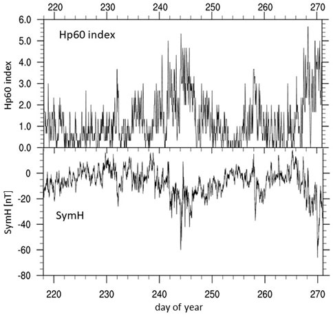
FIGURE 1. Geophysical conditions from August 5 (DOY 218) to September 26 (DOY 270) 2020: Hp60 index (top) and Sym/H [nT] (bottom).
The effect of the geomagnetic active period is visible in the F-region neutral wind at 250 km illustrated at geographic latitude λg = 30o for 12 UT in Figure 2 with the time and longitudinal variation indicated in the y- and x-direction, respectively. We label the simulation with tidal forcing at the lower boundary (LB) “with LB tides” (Figure 2A) and the simulation without tides at the LB “no LB tides” (Figure 2B.), the difference between the two simulations is labeled “only LB tides” (Figure 2C). The difference or the “only tides” case removes most of the effect from in situ generated tides due to the absorption of solar radiation in the F-region and from the geomagnetic forcing although some minor non-linear effects remain.
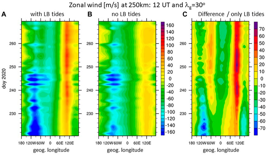
FIGURE 2. Zonal wind [m/s] at 250 km for 12 UT and geographic latitude λg = 30o for simulation (A) with tides at the lower boundary (LB), (B) without tides at the LB, (C) differences between (A) and (B) which isolates the effect of the LB tides.
The zonal wind clearly shows a diurnal variation with a strong zonal wave number 1 in the case “with LB tides” and “no LB tides”. However, in the case “with LB tides” higher order zonal wave numbers develop after approximately DOY 230 within a few days as visible in the longitudinal variation. This rapid transition, happening between approximately DOY 232 and DOY 238, is even more apparent in the “only tides” case in Figure 2C. In the following, we will focus on DOY 220–270 period to investigate how the lower atmospheric tides can facilitate this change. Note that the neutral wind in Figure 2 is depicted at a constant universal time (UT) and therefore the longitudinal axis corresponds to solar local time (SLT).
It is important to examine that the model in general reproduces the observed variation in the zonal wind at 250 km altitude. The ICON observatory samples all local times at each orbit but not for all longitudes and latitudes. We therefore average data using a 30 days sliding window between 25o to 40o geographic latitude (λg) to determine a longitudinal mean zonal wind over DOY and SLT. The model is sampled at the location of MIGHTI vector winds with the best quality flag. The model and data are processed in the same way. Figure 3 depicts the MIGHTI zonal wind (3a) and the MIGHTI-sampled TIEGCM zonal winds (3b) at 250 km.
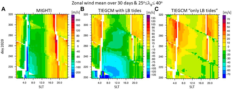
FIGURE 3. Zonal wind [m/s] at 250 km averaged over 30 days and between geographic latitudes λg of 25o ≤ λg ≤ 40o (A). MIGHTI zonal wind, (B). TIEGCM with LB tides sampled as MIGHTI winds, (C). TIEGCM only due to LB tides.
The diagonal lines in Figure 3 are an indication that longitudes are not equally sampled in the 30 days window (Cullens et al., 2020). The observations (Figure 3A) experience larger variations than the model (Figure 3B) and therefore, the color scale is adapted. This is not surprising, as first, the model is not perfect and secondly, even a perfect model could not reproduce the observed variations since it is forced by time averaged tidal variations. Even though the zonal wind magnitude is not the same, the variations with local time and over day of year are similar. The model (Figure 3B) exhibits more westward wind in the morning between DOY 200–230, compared to the observations, which becomes less westward with increasing DOY. In the late afternoon the observed zonal wind is eastward with the wind magnitude increasing with DOY, especially in the early evening (approximately 18–20 SLT). The model exhibits a similar variation with the zonal wind getting more eastward with increasing DOY. In general, the simulated zonal wind tends to be more westward than the observed one, but displays similar local time and DOY variations.
We established that the model captures the prevalent local time and DOY variations of the MIGHTI zonal wind. Therefore, we will use the model to isolate the effect of upward propagating tides on the noted wind changes (Figure 2). We examine the difference between the simulation with HME LB tides and without HME LB tides illustrated in Figure 3C. An increase in the semidiurnal component of the zonal wind with increasing DOY is visible in Figure 3C with approximate early morning and evening peaks. Note that signals of non-migrating tides are small since we average over almost all longitudes. In the following, tidal components for the “only LB tides” case will be illustrated and labels by (⋅)*. We note that we first take the difference between the simulations before determining the tidal components via a 2D Fast Fourier transformation (FFT) using a 2 days window.
To better understand the illustrated changes in the zonal wind in Figure 2C occurring after approximately DOY 232 we examine the changes in several tidal components in the following. Figure 4A depicts the migrating SW2* at 110 km with a maximum amplitude of roughly 45 m/s at middle latitudes. Figure 4B also shows SW2* but at 250 km, illustrating that between DOY 220 to approximately DOY 230 the latitudinal structure of SW2* at 110 km and 250 km are similar with the distinct middle latitude peaks in each hemisphere. After approximately DOY 232 the latitudinal structure is evolving differently at 250 km compared to 110 km. At 250 km the SW2* latitudinal structure is changed from the two middle latitude peaks to a single maximum amplitude peak at low latitude (Figure 4B).
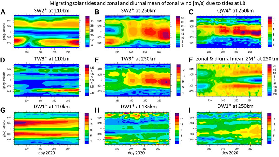
FIGURE 4. Amplitudes of migrating solar tides in zonal wind [m/s] only due to tides at lower boundary (LB) in (A). SW2 at 110 km and (B). SW2 at 250 km, (C). QW4 at 250 km, (D). TW3 at 110 km and (E). TW3 at 250 km, (G). DW1 at 110 km, (H). DW1 at 135 km, and (I). DW1 at 250 km, and (F). zonal and diurnal mean zonal mean wind at 250 km over geographic latitude and day of year (DOY) 2020.
The migrating quaddiurnal QW4* tide is not included in the HME LB forcing but is present at 250 km in the zonal wind with maximum amplitudes around 6 m/s at low latitudes (Figure 4C). The temporal and latitudinal structures of QW4* and SW2* at 250 km are similar. Therefore, we suggest that it is generated by tide-tide interaction of DW1 x TW3 = [1,1] x [3,3] leading to [4,4] + [2,2] = QW4 + SW2. Some smaller contributions might come from SW2 x SW2 = [4,4] + [0,0] = QW4 + ZM. Several studies suggested the generation of quaddiurnal tides through self-interaction of the semidiurnal tide, e.g., in SABER/TIMED temperatures (Liu et al., 2015) and during SSW (Gong et al., 2021) as well as through the diurnal and terdiurnal non-linear interaction as observed in the upper thermosphere at Arecibo during the 2016 SSW (Gong et al., 2018). While QW4 can be excited by the non-linear interaction of SW3 x SW1 = [2,3] x [2,1] leading to [4,4] + [0,2], SW3 and SW1 amplitudes are relatively small in the simulation and this non-linear interaction is therefore excluded from our consideration.
The migrating terdiurnal tide TW3* is shown at 110 km and 250 km in Figures 4D, E, respectively. The terdiurnal tides are not included in the HME LB tidal specification. TW3* amplitudes are small at 110 km with a maximum of 4 m/s at middle latitudes, but TW3* amplitude is up to 19 m/s at 250 km with the maximum at very low latitudes. The TW3* at 250 km (Figure 4E) emulates very closely the latitudinal and time variation of SW2* (Figure 4B). With TW3* amplitudes being approximately 2/3 of SW2* amplitude we suggest that TW3* is generated mainly by DW1 x SW2 = [1,1] x [2,2] leading to [3,3] + [1,1] = TW3 + DW1. DW1 serves here as primary and secondary wave. Note that Figure 4 depicts the difference between a simulation with and without HME LB tidal forcing and therefore most in situ solar heating induced tides in the thermosphere are removed.
DW1* is depicted at 110 km (Figure 4G) and at 250 km (Figure 4I). At 250 km DW1* has a similar temporal variation equatorward of 30o geographic latitude as SW2* and TW3* with an amplitude peak around DOY 265, and minor peaks around 255 and 240. The importance of the DW1 x SW2 interaction is well accepted in the literature as an important source of TW3 (see, e.g., Moudden and Forbes, 2013, and references therein), although generally of secondary importance to direct thermal forcing. Ours is the first report of TW3 production in the thermosphere by this mechanism.
DW1* is strongly forced at the lower boundary as evidenced by its 10–18 m/s amplitudes at 110 km in Figure 4G. However, DW1 has a short vertical wavelength (≈30 km) and does not penetrate much above 110 km; see for instance, Figure 4H which indicates amplitudes of 4–8 m/s at 135 km and low latitudes after DOY 232. We conclude that the DW1* signature in Figure 4I is not the result of DW1 propagating upwards from the LB, but rather is excited in situ through non-linear interaction as noted above.
Finally, we note the intensification of zonal and diurnal mean (ZM*) zonal winds after DOY 232 at 250 km (Figure 4F) leading to wind magnitudes ranging from −20 to 15 m/s around DOY 260. We conclude that these are due to the momentum deposited into the background atmosphere of the intensified migrating tides DW1*, SW2*, TW3*, QW4* after DOY 232 which is supported by the change in latitudinal structure of ZM* after DOY 232 reflecting the strong change in SW2* and TW3* (Figures 4B, E). As noted by Angelats i Coll and Forbes (2002), through examination of Eliassen-Palm flux divergences, it is not unexpected to see regions of eastward acceleration (and therefore eastward ZM zonal winds) in connection with dissipation of westward-propagating waves.
In the following, we focus on DOY 265 when the migrating tides exhibit a peak at low latitudes at 250 km (see Figures 4B, C, E, I). In Figure 5 the latitude-height variations of tidal amplitudes in zonal and meridional wind at DOY 265 are depicted. Figures 5A–C show the DW1, SW2, and TW3 zonal wind amplitudes only due to in situ forcing without any upward propagating LB tides. These diagnostics will be helpful to assess the importance of upward propagating tides in comparison to the in situ forced components.
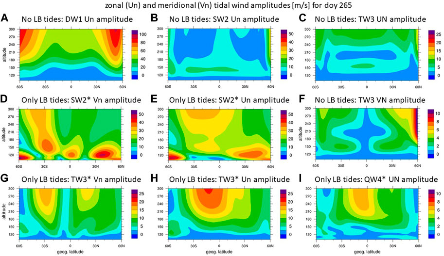
FIGURE 5. Amplitude of migrating solar tides in neutral wind [m/s] at DOY 265 over geographic latitude from the simulation with no LB tides (A). DW1 in zonal wind, (B). SW2 in zonal wind, (C). TW3 in zonal wind, (F). TW3 in meridional wind; and only due to tides at the LB (D). SW2 in meridional wind, (E). SW2 in zonal wind, (G). TW3 in meridional wind, (H). TW3 in zonal wind, (I). QW4 in zonal wind.
Figure 5A shows that the DW1 zonal wind component of the in situ solar EUV-driven circulation is strongest at middle to high latitudes (amplitudes of up to 80 m/s) and at low latitudes (equatorward of ±30° geographic latitude) has amplitudes of 40 m/s between 200 and 300 km. The in situ forced SW2 (Figure 5B) is very small with values less than 10 m/s over most of the domain. The SW2* amplitude from the upward propagating tides is around 30 m/s (Figure 5E) and much larger than the in situ driven SW2. SW2* due to upward propagating tides has almost the same magnitude as the in situ driven DW1 at low latitudes (Figure 5A). Thus, it is expected that SW2* due to upward propagating tides contributes significantly to the thermospheric circulation at these latitudes and altitudes.
Only a few studies (e.g., Forbes and Garrett, 1979; Forbes et al., 2011) investigated the relative importance of in situ vs. vertically-propagating semidiurnal tides to the dynamics of the upper thermosphere, finding that the major contribution comes from thermal excitation above 100 km except during solar minimum conditions when contributions from upward propagating semidiurnal tides can be comparable in magnitude. Forbes et al. (2011) fit HMEs to semidiurnal tidal temperatures derived from TIMED/SABER in the lower thermosphere, and compared the HME-extrapolated values with SW2 exosphere temperatures derived from CHAMP and GRACE densities near ∼400 km. The comparisons were made during the January-July 2004 (F10.7 ≈ 90-130sfu) and December 2005-July 2006 (F10.7 ≈ 75-100sfu) intervals, and revealed maxima during the Dec-Feb and Apr-Jul months. Interestingly, they concluded that the in situ contribution to SW2 dominated over any contribution propagating from below, opposite to the conclusion made above based on TIEGCM driven by HME LB tides. Unfortunately, no results from this study were available during September (i.e., DOY 265), and the present results moreover correspond to deeper solar minimum (F10.7 ≈ 70sfu), precluding any definitive conclusions based on comparisons between the two studies. Therefore, further work remains to be done on this aspect of thermosphere dynamics.
The depiction of TW3 meridional wind amplitude in Figure 5F can be contrasted against that in Figure 5G as further evidence for in situ generation of TW3* due to tide-tide interactions (recall that terdiurnal tides are not included in the LB forcing). Comparison between Figures 5H, C supports the same conclusion for the zonal wind component of TW3. We want to point out that the “no LB tides” depictions of tides (Figures 5A–C, F) are not based on simulation differences and therefore can show tidal signatures at high latitude induced by the offset of the aurora region with respect to the geographic coordinate system.
Surprisingly, maximum zonal wind amplitudes for TW3* (Figure 5H) are approaching those of SW2* (Figure 5E) at low latitudes and are approximately half of the in situ generated DW1 (Figure 5A). Noting the meridional wind amplitudes of order 10–20 m/s for both SW2* (Figure 5D) and TW3* (Figure 5G) around ±20–30° latitude, from which we conclude that their combined effects on field-align plasma transport may be significant.
Finally, QW4* is plotted in Figure 5I, indicating amplitudes of order 8 m/s. While significantly smaller than its SW2* and TW3* counterparts in Figures 5E, H, respectively, it is nevertheless noteworthy in terms of its obvious origins of tide-tide non-linear interactions.
The evolution of SW2* structures as evident in the presented TIEGCM-ICON simulation (e.g., Figure 4B) is one reason why this time period is so interesting. In the presented case, we wish to consider the height evolution of the latitude structures as well and connecting the latitude vs. DOY evolutions of SW2* U at 110 km and 250 km (Figures 4A, B, respectively). The HMEs are useful in providing that interpretation. We use the tidal fitting to a minimum number of HMEs to capture the simulated SW2 structure. The resulting SW2 zonal wind amplitude illustrated in Figures 6C, D represents the upward propagating tidal component. The height vs. latitude structures of SW2* U at DOY 224 and DOY 265 (Figures 6A, B) will be interpreted with the help of HMEs (Figures 4A, B). The corresponding illustration to Figure 6 for SW2* meridional wind at DOY 224 and DOY 265 is given in Supplementary Figure S1.
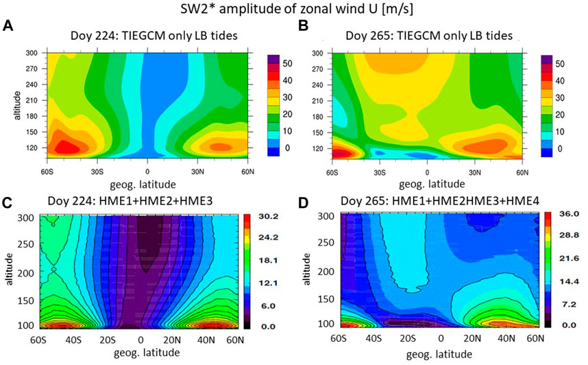
FIGURE 6. Amplitude of semidiurnal migrating tides for zonal wind [m/s] for DOY 224 [left panels (A, C)] and DOY 265 [right panels (B, D)] based on TIEGCM only due to LB tides [(top panels (A, B)] and HME fitting with the least HMEs: 3 modes for DOY 224 (c.) and 4 modes for DOY 265 (D).
In general, it was determined that the height vs. latitude structures of tides are well represented by the superimposed latitude-height structures of combined HME1, HME2, HME3, and HME4 (Cullens et al., 2020; Forbes et al., 2022). Therefore, reconstructions based on various combinations of HMEs can be performed, and those that assumed the greatest role in accounting for the simulated TIEGCM-ICON structures can be identified. It is important to note that these HMEs (1–4) have vertical wavelengths (λz) entering the thermosphere of ≳300 km, ∼85 km, ∼57 km, ∼40 km, respectively, and that the longer the λz the more effectively that HME penetrates to, say, 250 km.
It was found that for DOY 224, the dominant HME was the first antisymmetric HME2 (Supplementary Figure S2B), which accounts for the double-maxima in latitude occurring at both 110 km and 250 km for zonal wind U in Figure 6A. Unequal peaks between hemispheres at both heights are accounted for by interference with the symmetric mode HME3 and HME1 and/or HME4. Adding HME4 does not seem to make it agree better with TIEGCM results and the reconstruction using the combination of HME1, HME2, and HME3 for the zonal wind captures the salient latitude-height variations in the TIEGCM-ICON SW2* Figures 6A, C).
For the period after about DOY 240 at 250 km, all HMEs play a role as can be seen in the reconstruction in Figure 6D and the HME amplitudes in Supplementary Figures S2I, J, M, N. For zonal wind U, HME3 reinforces HME1 in the equatorial region above approximately 150 km, and nearly cancels HME1 at higher latitudes above 150 km, resulting in a more restricted latitude extent of the total response. Below 150 km the behavior of the combined HME1 and HME3 is reversed with an almost cancellation in the equatorial region and two maxima at high latitudes. HME2 and HME4 both contribute to the pronounced asymmetries at 250 km and 110 km (Supplementary Figure S2). All of the HMEs play a non-negligible role at 110 km and 250 km. The stark difference in the importance of the HME modes at DOY 224 with a dominant asymmetric HME2 versus DOY 265 with HME1 to HME4 all playing a role has probably its origin the middle atmosphere where antisymmetric modes can be excited as discussed in the introduction.
In the following, we examine the effect of significant dynamical changes during this period on the mean ionosphere-thermosphere state, specifically the NmF2 and composition via O/N2. First, we evaluate the simulated NmF2, which we do by comparing to FORMOSAT-7/COSMIC-2 (COSMIC-2) observations (Schreiner et al., 2020). COSMIC-2 was launched in June 2019 and consists of 6 satellites in low 24o inclination orbits with GNSS-radio occultation payload providing more than 4,000 high-quality electron density profiles per day. We are using RO Level 2 data product “ionPrf” which contains the ionospheric electron density profiles validated by Cherniak et al. (2021).
We use the maximum electron density (Ne) in the “ionPrf” data files if the associated altitude is at least 200 km, which eliminates instances of capturing sporadic E occurrence. In the following, we use the maximum Ne as a measure of NmF2, which is a reasonable approximation since the major part of the vertical extent of the F-region is sampled. The maximum Ne observations between 11 SLT to 18 SLT are binned by DOY and by 2.5o in quasi dipole latitude. Figure 7A illustrates the median of the maximum Ne in each bin. Note that the median is chosen to reduce the effect of outliers, however in our case using the average of the maximum Ne of each bin leads to very similar variations. Since the COSMIC-2 constellation was not spread evenly during this early mission phase, there is a longitudinal bias with respect to quasi-dipole latitude in the data (see Supplementary Figure S4). The negative quasi-dipole latitudes are preferably sampled in the African-Asian sector where the magnetic equator is in the northern hemisphere and therefore, the orbit dips to lower quasi-dipole latitudes than in the Pacific-American sector. However, this longitudinal bias does not explain the larger median Ne values in the northern than southern EIA crest (Figure 7A.) since even when restricting the geographic longitudes to the African-Asian sector a north-south differences in median Ne magnitude remains. We conclude that the north-south asymmetry in the EIA is not an artifact of the data sampling and processing.
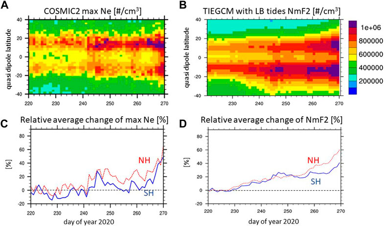
FIGURE 7. Top panels (A). Median of maximum electron density from COSMIC2 RO (equivalent to NmF2) and (B) average of NmF2 from TIEGCM with LB tides [1/cm3] for binned values (bin size 1 day and 2.5o quasi dipole latitude); bottom panels: relative change of quasi dipole latitudinal average between 5o ≤ |λqd| ≤ 20o of (C) maximum electron density from COSMIC and (D) NmF2 from TIEGCM with respect to average latitudinal variation between DOY 220–225.
The TIEGCM simulation with HME LB tides is binned like the observations with the difference of using NmF2 and all available longitudes (Figure 7B). In the model the southern part of the EIA is larger than the northern part, which is opposite to the observations (Figure 7A). The study period starts just 40 days after solstice and therefore the influence of northern hemisphere summer conditions are reflected in the observations with larger northern than southern EIA, but the difference reverses around October (e.g., Burns et al., 2012). The TIEGCM can in general reproduce the hemispheric difference in the EIA strength (e.g., Maute, 2017). However, in the current case the model lacks representing the hemispheric difference. This apparent model bias needs further examination which is beyond the scope of the current study.
Both observations and model exhibit an increase in NmF2 with DOY. To compare the temporal variation, we average the NmF2 over 5o ≤ |λqd| ≤ 20o with quasi dipole latitude λqd in both hemispheres and reference to the 5days-average of DOY 220–224 to remove the baseline bias. Figures 7C, D depict the relative change of NmF2 for the observations and simulation, respectively, with an increase after DOY 240 in the observations and after approximately DOY 235 in the simulation. The temporal variation of simulated average NmF2 in the northern EIA crest compares better with the observations than in the southern hemisphere crest. In the southern hemisphere, the observed relative changes of maximum Ne are smaller than in the simulation. We should note that signals of geomagnetic activity are visible around DOY 244, DOY 258, and DOY 268 in the observation and the model (Figures 7A, B). Overall, the simulation can reproduce the salient temporal variation of observed NmF2 and therefore, it will be used to examine the contribution of the LB tides to this temporal variation.
Figure 8A illustrates the zonal and diurnal mean change in NmF2 due to LB tides with respect to the simulation without LB tides. We note that the simulation without LB tides includes the effect of geomagnetic forcing while the “only LB tides” case does not, and therefore there are slight decreases in the percent changes during the geomagnetic active times (Figure 8A). The overall changes are negative and increase significantly with time, especially after DOY 235. At low latitudes a decrease of approximately 15%–20% compared to the beginning of the period can be attributed to the effect of LB tides. To provide more details of the relative changes in NmF2 (Figure 8A), we illustrated the increase in NmF2 over the time period with respect to DOY 220 for the simulation with and without LB tides (Supplementary Figures S5A, B, respectively). The magnitude of the temporal changes in NmF2 after approximately DOY 235 are different between the two simulations with a strong increase in NmF2 occurring in the simulation without LB tides while the simulation with LB tides exhibits a very modest increase, which leads to the negative change in NmF2 in the “only LB tide” case (Figure 8A).
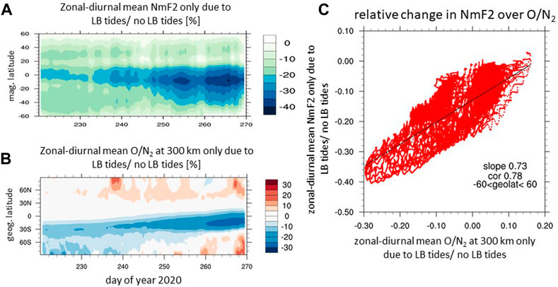
FIGURE 8. Time evolution of the relative change in the zonal and diurnal mean (A). NmF2 over quasi dipole latitude and (B) O/N2 ratio at 300 km over geographic latitude due to lower atmospheric tidal forcing with respect to no tidal forcing; (C) correlation between relative NmF2 change and O/N2 equatorward of |λm| ≤ 60o and |λg| ≤ 60o, respectively for the time window.
Part of the decrease in NmF2 is related to compositional changes which can be approximated by O/N2 at 300 km. Figure 8B illustrates the relative change of the zonal and diurnal mean O/N2 for the “only LB tides” case with respect to the “no LB tide” case. The mean O/N2 is decreasing by approximately 10% compared to the beginning of the time period. Supplementary Figure S5 illustrates that the zonal and diurnal mean O/N2 at 300 km is decreasing in the simulation with LB tides, especially after DOY 235 (Supplementary Figure S5C), but the low latitude maximum O/N2 is almost constant with time in the simulation without LB tides (Supplementary Figure S5D). The similar timing of the O/N2 changes and of the migrating tides and background wind (Figure 4) in the simulation with LB tides strongly suggest that the dynamical and compositional changes are connected.
These results indicate that the decrease in O/N2 due to LB tides partly compensate for the seasonal increase in NmF2 (Figure 8B) and therefore leads to a smaller increase in NmF2 with DOY in the simulation with LB tides compared to without LB tides (Supplementary Figures S5A, B, respectively). The relative change of the mean NmF2 in the “only LB tides” case has a strong correlation to the relative change of the mean O/N2 at 300 km (Figure 8C). The difference in the NmF2 latitudinal variation in Supplementary Figures S5A, B suggests that there are additional contributions from the low latitude ExB drift and the meridional wind leading to EIA differences, such as the EIA position at higher magnetic latitude and with less hemispheric difference in the simulation with LB tides than without. However, the simulation suggests that the main contribution to the temporal changes in NmF2 and O/N2 are due to the dynamical changes associated with the LB forcing since no strong temporal variation in the EIA location and hemispheric difference was identified. Note that the daytime NmF2 dominates the diurnal mean NmF2.
This study focuses on the DOY 220–270, 2020 time period which exhibits significant temporal and spatial changes in the migrating solar tides as captured by the TIEGCM-ICON driven by the observationally based ICON-HME tides. The ICON mission provides TIEGCM simulations forced at its 97 km lower boundary with and without HME tides. This set of simulations enables us to quantify the effect of upward propagating tides, specifically the impact of the significant temporal and spatial tidal changes, on the lower and upper thermosphere and the ionosphere.
While strong SW2 changes were observed and simulated before and associated with the equinox transitions (e.g., Conde et al., 2018; Pedatella et al., 2021), these studies focused on the mesosphere and lower thermosphere. To our knowledge the current study is the first report of the effects of the strong sudden changes in SW2 on the upper thermosphere and ionosphere. Equinox transitions in the thermosphere are complex since they are influenced by the combined effect of transition characteristics in different altitude regions. During the DOY 220–270, 2020 study period the large tidal changes start 34 days before September equinox (DOY 266). We do not speculate about potential connection to equinox transition, but rather focus on the dynamical changes and its associated effect on composition and plasma distribution. We summarize our main findings.
• The latitudinal structure of SW2 amplitude in zonal wind at 250 km is changing quickly within approximately 8 days after DOY 232 from mid-latitudes peaks in either hemisphere to one broad low latitude peak. The change in SW2 latitudinal structure is associated with the increasing importance of antisymmetric HMEs after DOY 240 when HME1, HME2, HME3, HME4, corresponding to (2,2), (2,3), (2,4), (2,5), respectively, are of comparable size, while before DOY 232 HME1, HME2, HME3, corresponding to (2,2), (2,3), and (2,4), are important with HME2 (2,3) having the largest amplitude.
Studies showed that mean zonal wind condition changes in the middle atmosphere influence the propagation of different Hough Modes (e.g., Hagan et al., 1992; Xu et al., 2010). Therefore, the significant changes in the prevalence of different Hough Mode components during the study period is indicative of changes in the middle atmosphere. Due to the vertical coupling of the middle to upper atmosphere, the strong upper thermospheric tidal changes occur within approximately 8 days.
The simulation indicates that the upward propagating SW2 is more important that the in situ forced SW2 in the upper thermosphere during the study period. Previous results by Forbes et al. (2011) for solar medium conditions and December to July season demonstrated than the in situ forced SW2 dominates over the propagating SW2 component. Further studies are necessary to understand this difference.
• The latitudinal structure of migrating tides during this time periods is strongly modified at 250 km compared to 110 km. The temporal and latitudinal variation of SW2 is imprinted on the migrating tides, DW1, TW3, and QW4. In the simulations, the terdiurnal and quaddiurnal tides are generated internally since only diurnal and semidiurnal tides are included in the lower boundary forcing.
QW4 is the smallest of the migrating tides and might be generated by non-linear interaction between DW1xTW3 as well as some contribution might come from SW2xSW2. TW3 amplitudes at 250 km are large, approximately 2/3 of SW2. The simulation indicates it is generated by the non-linear interaction between DW1xSW2 in the upper thermosphere. While this non-linear interaction is well documented in the lower thermosphere, to our knowledge, its importance for the upper thermosphere was not noted before. Since both SW2 and TW3 in the meridional wind are strong at 250 km, it is conceivable that they play an important role for field-aligend plasma drift.
• Associated with the changes in SW2 and the other migrating tides, the background winds are significantly changed within approximately 8 days, suggesting that dissipating migrating tides deposited their momentum into the background atmosphere. Angelats i Coll and Forbes (2002) found that dissipation of westward propagating tides can create eastward accelerations of mean zonal wind at some latitudes.
These dynamical changes influence the composition and the plasma distribution. The simulation results indicate that during the time period a 15%–20% change in the zonal and diurnal mean NmF2 is associated with the strong tidal and background changes during this time period. The mean change in NmF2 is strongly aligned with the modification of roughly 10% in the composition as approximated by O/N2 during this time period.
To set the compositional and plasma density changes during DOY 220–270, 2020 period in perspective, we compare with some previous studies. Jones Jr. et al. (2014) used the TIEGCM forced with and without Climatological Tidal Model of Thermosphere (CTMT) (Oberheide et al., 2011a) to delineate the effect of upward propagating tides on the TI system. They find a 20% decrease in NmF2 and 4% decrease in [O]/[N2] due to the inclusion of tides with respect to the simulation without tides in August-September but no strong change within days or even 40 days. Similarly, Maute (2017) using the TIEGCM driven by daily varying LB tides smoothed by a 27 days running mean of the Thermosphere-Ionosphere-Mesosphere-Electrodynamic GCM (TIMEGCM) did not see the strong changes in the SW2 reported in this study. This highlights that the change we report here is much stronger than expected from seasonal and climatological behavior.
The study period clearly demonstrates the effect of strong and sudden tidal and mean circulation changes on the upper thermosphere and ionosphere. However, the study has uncertainties due to the limited data coverage. While ICON provides unique observations to study the vertical coupling effects on the thermosphere and ionosphere, atmospheric tides described by HME are based on 10S-40N observations within an up to 41 days window. More frequent sampling of all latitudes, local times, and longitudes are crucial to capture higher order symmetric and antisymmetric HME modes without ambiguity and with higher temporal cadence. Future missions like DYNAMIC (National Research Council, Solar and space physics: a science for a technological society, 2013) will provide tidal specification on a shorter time scale and therefore can provide new insight into their temporal and spatial variations.
The solar wind parameters are available from the NASA/GSFC’s Space Physics Data Facility’s OMNIWeb service at https://omniweb.gsfc.nasa.gov/ow min.html. The Hp60 index (Matzka et al., 2022) is available at Geoforschungszentrum Potsdam (GFZ), Germany via https://kp.gfz-potsdam.de/en/hp30-hp60/data. COSMIC Level 2 “ionPrf” product is provided by COSMIC Data Analysis and Archive Center (CDAAC) available via https://doi.org/10.5065/t353-c093. We used the “ionPrf” files of ionospheric electron density profiles. The ICON mission data is available at Goddard Space Flight Center Space Physics Data Facility (SPDF) https://cdaweb.gsfc.nasa.gov/ and at the Space Science Laboratary (SSL) ftp server ftp://icon576 science.ssl.berkeley.edu/pub. The ICON-MIGHTI neutral wind vectors Level 2.1 V05 data can be found at SSL ftp server under Level2/MIGHTI/2020/DOY/ZIP/ICON L2-1 MIGHTI 2020 MM-DD v05r000.ZIP). The ICON-HME product Level4 V02 can be found at SSL ftp server under Level4/HME/2020/ZIP/ICON L4-1 HME 2020-MM-DD v02r004.ZIP. The TIEGCM-ICON simulations Level 4 V01 are available at ftp://icon-science.ssl.berkeley.edu/pub with HME LB forcing at Level4/TIEGCM/2020/ZIP/ICON L4-3 TIEGCM 2020 MM-DD v01r000.ZIP and without HME LB forcing Level4/TIEGCM-NOHME/2020/ZIP/ICON L4-3 TIEGCM-NOHME 2020 MM584 DD v01r000.ZIP.
AM conducted the analysis. CC and JF conducted the HME analysis. AM and JF drafted the manuscript. AM, JF, CC, TI worked on the interpretation of the analysis.
AM is supported by ICON NASA grant 80NSSC21K1990. JF and CC were supported by the ICON mission through NASA Explorers Program contracts NNG12FA45C and NNG12FA42I. We would like to acknowledge high-performance computing support from Cheyenne (doi:10.5065/D6RX99HX) provided by NCAR’s Computational and Information Systems Laboratory, sponsored by the National Science Foundation. This material is based upon work supported by the National Center for Atmospheric Research, which is a major facility sponsored by the National Science Foundation under Cooperative Agreement No. 1852977.
AM would like to thank Dr. N. Pedatella for comments on an earlier draft.
The authors declare that the research was conducted in the absence of any commercial or financial relationships that could be construed as a potential conflict of interest.
All claims expressed in this article are solely those of the authors and do not necessarily represent those of their affiliated organizations, or those of the publisher, the editors and the reviewers. Any product that may be evaluated in this article, or claim that may be made by its manufacturer, is not guaranteed or endorsed by the publisher.
The Supplementary Material for this article can be found online at: https://www.frontiersin.org/articles/10.3389/fspas.2023.1147571/full#supplementary-material
Akmaev, R. A. (2001). Seasonal variations of the terdiurnal tide in the mesosphere and lower thermosphere: A model study. Geophys. Res. Lett. 28, 3817–3820. doi:10.1029/2001GL013002
Angelats i Coll, M., and Forbes, J. M. (2002). Nonlinear interactions in the upper atmosphere: The s = 1 and s = 3 nonmigrating semidiurnal tides. J. Geophys. Res. 107, SIA 3-1–SIA 3-15. doi:10.1029/2001JA900179
Azeem, I., Walterscheid, R. L., Crowley, G., Bishop, R. L., and Christensen, A. B. (2016). Observations of the migrating semidiurnal and quaddiurnal tides from the RAIDS/NIRS instrument. J. Geophys. Res. Space Phys. 121, 4626–4637. doi:10.1002/2015JA022240
Burns, A. G., Solomon, S. C., Wang, W., Qian, L., Zhang, Y., and Paxton, L. J. (2012). Daytime climatology of ionospheric NmF2 and hmF2 from COSMIC data. J. Geophys. Res. Space Phys. 117. doi:10.1029/2012ja017529
Butler, S., and Small, K. (1963). The excitation of atmospheric oscillations. Proc. R. Soc. Lond. Ser. A. Math. Phys. Sci. 274, 91–121.
Cherniak, I., Zakharenkova, I., Braun, J., Wu, Q., Pedatella, N., Schreiner, W., et al. (2021). Accuracy assessment of the quiet-time ionospheric F2 peak parameters as derived from COSMIC-2 multi-GNSS radio occultation measurements. J. Space Weather Space Clim. 11, 18. doi:10.1051/swsc/2020080
Conde, M. G., Bristow, W. A., Hampton, D. L., and Elliott, J. (2018). Multiinstrument studies of thermospheric weather above Alaska. J. Geophys. Res. Space Phys. 123, 9836–9861. doi:10.1029/2018JA025806
Conte, J. F., Chau, J. L., Laskar, F. I., Stober, G., Schmidt, H., and Brown, P. (2018). Semidiurnal solar tide differences between fall and spring transition times in the northern hemisphere. Ann. Geophys. 36, 999–1008. doi:10.5194/angeo-36-999-2018
Conte, J. F., Chau, J. L., Stober, G., Pedatella, N., Maute, A., Hoffmann, P., et al. (2017). Climatology of semidiurnal lunar and solar tides at middle and high latitudes: Interhemispheric comparison. J. Geophys. Res. Space Phys. 122, 7750–7760. doi:10.1002/2017JA024396
Cullens, C., Immel, T. J., Triplett, C. C., Yen-Jung, W., England, S. L., Forbes, J. M., et al. (2020). Sensitivity study for ICON tidal analysis. Prog. Earth Planet. Sci. 7, 18. doi:10.1186/s40645-020-00330-6
Cullens, C. Y., England, S. L., Immel, T. J., Maute, A., Harding, B. J., Triplett, C. C., et al. (2022). Seasonal variations of medium-scale waves observed by icon-mighti. Geophys. Res. Lett. 49, e2022GL099383. doi:10.1029/2022gl099383
Dhadly, M. S., Englert, C. R., Drob, D. P., Emmert, J. T., Niciejewski, R., and Zawdie, K. A. (2021). Comparison of ICON/MIGHTI and TIMED/TIDI neutral wind measurements in the lower thermosphere. J. Geophys. Res. Space Phys. 126, e2021JA029904. doi:10.1029/2021ja029904
Drob, D. P., Emmert, J. T., Crowley, G., Picone, J. M., Shepherd, G. G., Skinner, W., et al. (2008). An empirical model of the earth’s horizontal wind fields: HWM07. J. Geophys. Res. Space Phys. 113. doi:10.1029/2008ja013668
Du, J., and Ward, W. (2010). Terdiurnal tide in the extended canadian middle atmospheric model (CMAM. J. Geophys. Res. Atmos. 115. doi:10.1029/2010jd014479
Emery, B., Roble, R., Ridley, E., Richmond, A., Knipp, D., Crowley, G., et al. (2012). Parameterization of the ion convection and the auroral oval in the NCAR thermospheric general circulation models. Tech. rep. Boulder CO, USA: National Center for Atmospheric Research. doi:10.5065/D6N29TXZ
England, S. L., Englert, C. R., Harding, B. J., Triplett, C. C., Marr, K., Harlander, J. M., et al. (2022). Vertical shears of horizontal winds in the lower thermosphere observed by ICON. Geophys. Res. Lett. 49, e2022GL098337. doi:10.1029/2022gl098337
Englert, C. R., Harlander, J. M., Brown, C. M., Marr, K. D., Miller, I. J., Stump, J. E., et al. (2017). Michelson interferometer for global high-resolution thermospheric imaging (MIGHTI): Instrument design and calibration. Space Sci. Rev. 212, 553–584. doi:10.1007/s11214-017-0358-4
Fesen, C. G., Roble, R. G., and Ridley, E. C. (1991). Thermospheric tides at equinox: Simulations with coupled composition and auroral forcings: 2. Semidiurnal component. J. Geophys. Res. Space Phys. 96, 3663–3677. doi:10.1029/90JA02189
Forbes, J. M. (1982a). Atmospheric tide: 2. The solar and lunar semidiurnal components. J. Geophys. Res. 87, 5241–5252. doi:10.1029/JA087iA07p05241
Forbes, J. M. (1982b). Atmospheric tides: 1. Model description and results for the solar diurnal component. J. Geophys. Res. 87, 5222–5240. doi:10.1029/JA087iA07p05222
Forbes, J. M., and Garrett, H. B. (1978). Seasonal-latitudinal structure of the diurnal thermospheric tide. J. Atmos. Sci. 35, 148–159. doi:10.1175/1520-0469(1978)035<0148:slsotd>2.0.co;2
Forbes, J. M., and Garrett, H. B. (1979). The solar cycle variability of diurnal and semidiurnal thermospheric temperatures. J. Geophys. Res. Space Phys. 84, 1947–1949. doi:10.1029/ja084ia05p01947
Forbes, J. M., Oberheide, J., Zhang, X., Cullens, C., Englert, C. R., Harding, B. J., et al. (2022). Vertical coupling by solar semidiurnal tides in the thermosphere from ICON/MIGHTI measurements. J. Geophys. Res. Space Phys. 127, e2022JA030288. doi:10.1029/2022ja030288
Forbes, J. M., Zhang, X., Bruinsma, S., and Oberheide, J. (2011). Sun-synchronous thermal tides in exosphere temperature from CHAMP and GRACE accelerometer measurements. J. Geophys. Res. Space Phys. 116. doi:10.1029/2011JA016855
Forbes, J. M., Zhang, X., Hagan, M. E., England, S. L., Liu, G., and Gasperini, F. (2017). On the specification of upward-propagating tides for ICON science investigations. Space Sci. Rev. 212, 697–713. doi:10.1007/s11214-017-0401-5
Forbes, J. M., and Zhang, X. (2022). Hough mode extensions (HMEs) and solar tide behavior in the dissipative thermosphere. J. Geophys. Res. Space Phys. 127, e2022JA030962. doi:10.1029/2022JA030962
Fuller-Rowell, T. J. (1998). The “thermospheric spoon”: A mechanism for the semiannual density variation. J. Geophys. Res. Space Phys. 103, 3951–3956. doi:10.1029/97JA03335
Geißler, C., Jacobi, C., and Lilienthal, F. (2020). Forcing mechanisms of the migrating quarterdiurnal tide. Ann. Geophys. 38, 527–544. doi:10.5194/angeo-38-527-2020
Geller, M. A. (1970). An investigation of the lunar semidiurnal tide in the atmosphere. J. Atmos. Sci. 27, 202–218. doi:10.1175/1520-0469(1970)027<0202:aiotls>2.0.co;2
Gong, Y., Ma, Z., Lv, X., Zhang, S., Zhou, Q., Aponte, N., et al. (2018). A study on the quarterdiurnal tide in the thermosphere at Arecibo during the February 2016 Sudden Stratospheric Warming event. Geophys. Res. Lett. 45 (13), 149. doi:10.1029/2018GL080422
Gong, Y., Xue, J., Ma, Z., Zhang, S., Zhou, Q., Huang, C., et al. (2021). Strong quarterdiurnal tides in the mesosphere and lower thermosphere during the 2019 Arctic Sudden Stratospheric Warming over mohe, China. J. Geophys. Res. Space Phys. 126, e2020JA029066. doi:10.1029/2020ja029066
Gong, Y., and Zhou, Q. (2011). Incoherent scatter radar study of the terdiurnal tide in the E- and F-region heights at Arecibo. Geophys. Res. Lett. 38. doi:10.1029/2011GL048318
Hagan, M. E., Burrage, M. D., Forbes, J. M., Hackney, J., Randel, W. J., and Zhang, X. (1999). GSWM-98: Results for migrating solar tides. J. Geophys. Res. 104, 6813–6827. doi:10.1029/1998JA900125
Hagan, M. E., and Forbes, J. M. (2002). Migrating and nonmigrating diurnal tides in the middle and upper atmosphere excited by tropospheric latent heat release. J. Geophys. Res. Atmos. 107. ACL 6–1–ACL 6–15. doi:10.1029/2001JD001236
Hagan, M. E., Maute, A., Roble, R. G., Richmond, A. D., Immel, T. J., and England, S. L. (2007). Connections between deep tropical clouds and the Earth’s ionosphere. Geophys. Res. Lett. 34, L20109. doi:10.1029/2007GL030142
Hagan, M., and Forbes, J. (2003). Migrating and nonmigrating semidiurnal tides in the upper atmosphere excited by tropospheric latent heat release. J. Geophys. Res. 108, 10–1029. doi:10.1029/2002ja009466
Hagan, M., Vial, F., and Forbes, J. (1992). Variability in the upward propagating semidiurnal tide due to effects of qbo in the lower atmosphere. J. Atmos. Terr. Phys. 54, 1465–1474. doi:10.1016/0021-9169(92)90153-c
Harding, B. J., Chau, J. L., He, M., Englert, C. R., Harlander, J. M., Marr, K. D., et al. (2021). Validation of ICON-MIGHTI thermospheric wind observations: 2. Green-Line comparisons to specular meteor radars. J. Geophys. Res. Space Phys. 126, e2020JA028947. doi:10.1029/2020ja028947
Harding, B. J., Makela, J. J., Englert, C. R., Marr, K. D., Harlander, J. M., England, S. L., et al. (2017). The MIGHTI wind retrieval algorithm: Description and verification. Space Sci. Rev. 212, 585–600. doi:10.1007/s11214-017-0359-3
Harding, B. J., Wu, Y.-J. J., Alken, P., Yamazaki, Y., Triplett, C. C., Immel, T. J., et al. (2022). Impacts of the january 2022 Tonga volcanic eruption on the ionospheric dynamo: ICON-MIGHTI and swarm observations of extreme neutral winds and currents. Geophys. Res. Lett. 49, e2022GL098577. doi:10.1029/2022gl098577
Heelis, R. A., Chen, Y.-J., Depew, M. D., Harding, B. J., Immel, T. J., Wu, Y.-J., et al. (2022). Topside plasma flows in the equatorial ionosphere and their relationships to F-Region winds near 250 km. J. Geophys. Res. Space Phys. 127, e2022JA030415. doi:10.1029/2022ja030415
Holton, J. (1975). “The dynamic meteorology of the stratosphere and mesosphere,” in Meteorological monograph 15 (United States: American Meteorological Society).
Huang, C. M., Zhang, S. D., and Yi, F. (2007). A numerical study on amplitude characteristics of the terdiurnal tide excited by nonlinear interaction between the diurnal and semidiurnal tides. Earth, planets space 59, 183–191. doi:10.1186/bf03353094
Huba, J., Maute, A., and Crowley, G. (2017). Sami3_ICON: Model of the ionosphere/plasmasphere system. Space Sci. Rev. 212, 731–742. doi:10.1007/s11214-017-0415-z
Immel, T. J., England, S., Mende, S., Heelis, R., Englert, C., Edelstein, J., et al. (2018). The ionospheric connection explorer mission: Mission goals and design. Space Sci. Rev. 214, 13. doi:10.1007/s11214-017-0449-2
Immel, T. J., Harding, B. J., Heelis, R. A., Maute, A., Forbes, J. M., England, S. L., et al. (2021). Regulation of ionospheric plasma velocities by thermospheric winds. Nat. Geosci. 14, 893–898. doi:10.1038/s41561-021-00848-4
Jacobi, C., Krug, A., and Merzlyakov, E. (2017). Radar observations of the quarterdiurnal tide at midlatitudes: Seasonal and long-term variations. J. Atmos. Solar-Terrestrial Phys. 163, 70–77. doi:10.1016/j.jastp.2017.05.014
Jones, M., Forbes, J. M., Hagan, M. E., and Maute, A. (2014). Impacts of vertically propagating tides on the mean state of the ionosphere-thermosphere system. J. Geophys. Res. Space Phys. 119, 2197–2213. doi:10.1002/2013JA019744
Lei, J., Zhu, Q., Wang, W., Burns, A. G., Zhao, B., Luan, X., et al. (2015). Response of the topside and bottomside ionosphere at low and middle latitudes to the October 2003 superstorms. J. Geophys. Res. Space Phys. 120, 6974–6986. doi:10.1002/2015JA021310
Lilienthal, F., Jacobi, C., and Geißler, C. (2018). Forcing mechanisms of the terdiurnal tide. Atmos. Chem. Phys. 18, 15725–15742. doi:10.5194/acp-18-15725-2018
Lindzen, R. S., and Chapman, S. (1969). Atmospheric tides. Space Sci. Rev. 10, 3–188. doi:10.1007/bf00171584
Lindzen, R. S., and Hong, S.-s. (1974). Effects of mean winds and horizontal temperature gradients on solar and lunar semidiurnal tides in the atmosphere. J. Atmos. Sci. 31, 1421–1446. doi:10.1175/1520-0469(1974)031<1421:eomwah>2.0.co;2
Liu, G., Janches, D., Lieberman, R. S., Moffat-Griffin, T., Fritts, D. C., and Mitchell, N. J. (2020). Coordinated observations of 8- and 6-hr tides in the mesosphere and lower thermosphere by three meteor radars near 60°s latitude. Geophys. Res. Lett. 47, e2019GL086629. doi:10.1029/2019gl086629
Liu, M., Xu, J., Yue, J., and Jiang, G. (2015). Global structure and seasonal variations of the migrating 6-h tide observed by SABER/TIMED. Sci. China Earth Sci. 58, 1216–1227. doi:10.1007/s11430-014-5046-6
Macotela, E. L., Clilverd, M., Renkwitz, T., Chau, J., Manninen, J., and Banyś, D. (2021). Spring-Fall asymmetry in VLF amplitudes recorded in the North Atlantic region: The Fall-effect. Geophys. Res. Lett. 48, e2021GL094581. doi:10.1029/2021GL094581
Makela, J. J., Baughman, M., Navarro, L. A., Harding, B. J., Englert, C. R., Harlander, J. M., et al. (2021). Validation of ICON-MIGHTI thermospheric wind observations: 1. Nighttime red-line ground-based fabry-perot interferometers. J. Geophys. Res. Space Phys. 126, e2020JA028726. doi:10.1029/2020ja028726
Mannucci, A. J., Verkhoglyadova, O. P., Tsurutani, B. T., Meng, X., Pi, X., Wang, C., et al. (2015). Medium-range thermosphere-ionosphere storm forecasts. Space 13, 125–129. doi:10.1002/2014SW001125
Matzka, J., Bronkalla, O., Kervalishvili, G., Rauberg, J., and Yamazaki, Y. (2022). Geomagnetic hpo index. GFZ Data Serv. 2022. doi:10.5880/Hpo.000
Maute, A. (2017). Thermosphere-ionosphere-electrodynamics general circulation model for the ionospheric connection explorer: TIEGCM-ICON. Space Sci. Rev. 212, 523–551. doi:10.1007/s11214-017-0330-3
Millward, G. H., Moffett, R. J., Quegan, S., Fuller-Rowell, T. J., and Moffett, R. J. (1996). Ionospheric F-2 layer seasonal and semiannual variations. J. Geophys. Res. Space Phys. 101, 5149–5156. doi:10.1029/95JA03343
Miyahara, S., and Forbes, J. M. (1991). Interactions between gravity waves and the diurnal tide in the mesosphere and lower thermosphere. J. Meteorological Soc. Jpn. Ser. II 69, 523–531. doi:10.2151/jmsj1965.69.5_523
Moudden, Y., and Forbes, J. M. (2013). A decade-long climatology of terdiurnal tides using TIMED/SABER observations. J. Geophys. Res. Space Phys. 118, 4534–4550. doi:10.1002/jgra.50273
Oberheide, J., Forbes, J. M., Zhang, X., and Bruinsma, S. L. (2011a). Climatology of upward propagating diurnal and semidiurnal tides in the thermosphere. J. Geophys. Res. 116. doi:10.1029/2011JA016784
Oberheide, J., Forbes, J. M., Zhang, X., and Bruinsma, S. L. (2011b). Wave-driven variability in the ionosphere-thermosphere-mesosphere system from TIMED observations: What contributes to the ”wave 4. J. Geophys. Res. 116. doi:10.1029/2010JA015911
Pancheva, D., Mukhtarov, P., and Andonov, B. (2009). Nonmigrating tidal activity related to the sudden stratospheric warming in the Arctic winter of 2003-2004. Ann. Geophys. 27, 975–987. doi:10.5194/angeo-27-975-2009
Pancheva, D., Mukhtarov, P., Hall, C., Smith, A., and Tsutsumi, M. (2021). Climatology of the short-period (8-h and 6-h) tides observed by meteor radars at Tromsø and svalbard. J. Atmos. Solar-Terrestrial Phys. 212, 105513. doi:10.1016/j.jastp.2020.105513
Pedatella, N. M., Liu, H.-L., Conte, J. F., Chau, J. L., Hall, C., Jacobi, C., et al. (2021). Migrating semidiurnal tide during the September equinox transition in the Northern Hemisphere. J. Geophys. Res. Atmos. 126. doi:10.1029/2020JD033822
Qian, L., Burns, A. G., Emery, B. A., Foster, B., Lu, G., Maute, A., et al. (2014). The NCAR TIE-GCM: A community model of the coupled thermosphere/ionosphere system. Model. Ionosphere-Thermosphere Syst. Geophys. Monogr. Ser 201, 73–83.
Richmond, A. (1995). Ionospheric electrodynamics using magnetic apex coordinates. J. Geomagnetism Geoelectr. 47, 191–212. doi:10.5636/jgg.47.191
Roble, R., and Ridley, E. (1987). An auroral model for the NCAR thermospheric general circulation model (TGCM). United States: Annales Geophysicae 5A, 369–382.
Schmidt, H., Brasseur, G., Charron, M., Manzini, E., Giorgetta, M., Diehl, T., et al. (2006). The HAMMONIA chemistry climate model: Sensitivity of the mesopause region to the 11-year solar cycle and CO2 doubling. J. Clim. 19, 3903–3931. doi:10.1175/jcli3829.1
Schreiner, W., Weiss, J., Anthes, R., Braun, J., Chu, V., Fong, J., et al. (2020). COSMIC-2 radio occultation constellation: First results. Geophys. Res. Lett. 47, e2019GL086841. doi:10.1029/2019GL086841
Smith, A. K., Pancheva, D. V., and Mitchell, N. J. (2004). Observations and modeling of the 6-hour tide in the upper mesosphere. J. Geophys. Res. Atmos. 109, D10105. doi:10.1029/2003JD004421
Smith, A. K. (2000). Structure of the terdiurnal tide at 95 km. Geophys. Res. Lett. 27, 177–180. doi:10.1029/1999GL010843
Smith, A., and Ortland, D. (2001). Modeling and analysis of the structure and generation of the terdiurnal tide. J. Atmos. Sci. 58, 3116–3134. doi:10.1175/1520-0469(2001)0583116:MAAOTS2.0.CO;2
Stevens, M., Englert, C., Harlander, J., Marr, K., Harding, B., Triplett, C., et al. (2022). Temperatures in the upper mesosphere and lower thermosphere from o2 atmospheric band emission observed by icon/mighti. Space Sci. Rev. 218, 67–32. doi:10.1007/s11214-022-00935-x
Stevens, M. H., Englert, C. R., Harlander, J. M., England, S. L., Marr, K. D., Brown, C. M., et al. (2018). Retrieval of lower thermospheric temperatures from O2 A band emission: The MIGHTI experiment on ICON. Space Sci. Rev. 214, 4–9. doi:10.1007/s11214-017-0434-9
Stober, G., Kuchar, A., Pokhotelov, D., Liu, H., Liu, H.-L., Schmidt, H., et al. (2021). Interhemispheric differences of mesosphere–lower thermosphere winds and tides investigated from three whole-atmosphere models and meteor radar observations. Atmos. Chem. Phys. 21, 13855–13902. doi:10.5194/acp-21-13855-2021
Teitelbaum, H., Vial, F., Manson, A., Giraldez, R., and Massebeuf, M. (1989). Non-linear interaction between the diurnal and semidiurnal tides: Terdiurnal and diurnal secondary waves. J. Atmos. Terr. Phys. 51, 627–634. doi:10.1016/0021-9169(89)90061-5
Teitelbaum, H., and Vial, F. (1991). On tidal variability induced by nonlinear interaction with planetary waves. J. Geophys. Res. Space Phys. 96, 14169–14178. doi:10.1029/91JA01019
van Caspel, W. E., Espy, P. J., Hibbins, R. E., and McCormack, J. P. (2020). Migrating tide climatologies measured by a high-latitude array of SuperDARN HF radars. Ann. Geophys. 38, 1257–1265. doi:10.5194/angeo-38-1257-2020
Venkateswara Rao, N., Espy, P. J., Hibbins, R. E., Fritts, D. C., and Kavanagh, A. J. (2015). Observational evidence of the influence of Antarctic stratospheric ozone variability on middle atmosphere dynamics. Geophys. Res. Lett. 42, 7853–7859. doi:10.1002/2015GL065432
Volland, H. (1988). Atmospheric tidal and planetary waves. Berlin, Germany: Springer Science and Business Media.
Walterscheid, R., and Venkateswaran, S. (1979a). Influence of mean zonal motion and meridional temperature gradients on the solar semidiurnal atmospheric tide: A spectral study. Part I: Theory. J. Atmos. Sci. 36, 1623–1635. doi:10.1175/1520-0469(1979)036<1623:iomzma>2.0.co;2
Walterscheid, R., and Venkateswaran, S. (1979b). Influence of mean zonal motion and meridional temperature gradients on the solar semidiurnal atmospheric tide: A spectral study. Part II: Numerical results. J. Atmos. Sci. 36, 1636–1662. doi:10.1175/1520-0469(1979)036¡1636:IOMZMA¿2.0.CO;2
Ward, W., Seppälä, A., Yiğit, E., Nakamura, T., Stolle, C., Laštovička, J., et al. (2021). Role of the sun and the middle atmosphere/thermosphere/ionosphere in climate (rosmic): A retrospective and prospective view. Prog. Earth Planet. Sci. 8, 47–38. doi:10.1186/s40645-021-00433-8
Weimer, D. R. (2005). Improved ionospheric electrodynamic models and application to calculating Joule heating rates. J. Geophys. Res. 110, A05306. doi:10.1029/2004JA010884
Xu, J., Smith, A. K., Jiang, G., and Yuan, W. (2010). Seasonal variation of the hough modes of the diurnal component of ozone heating evaluated from aura microwave limb sounder observations. J. Geophys. Res. Atmos. 115, D10110. doi:10.1029/2009JD013179
Yamazaki, Y., Matzka, J., Stolle, C., Kervalishvili, G., Rauberg, J., Bronkalla, O., et al. (2022). Geomagnetic activity index hpo. Geophys. Res. Lett. 49, e2022GL098860. doi:10.1029/2022gl098860
Younger, P. T., Pancheva, D., Middleton, H. R., and Mitchell, N. J. (2002). The 8-hour tide in the arctic mesosphere and lower thermosphere. J. Geophys. Res. Space Phys. 107, SIA 2-1–SIA 2-11. doi:10.1029/2001JA005086
Keywords: migrating solar tides, tide-tide interaction, hough modes, composition, plasma distribution, vertical coupling
Citation: Maute A, Forbes JM, Cullens CY and Immel TJ (2023) Delineating the effect of upward propagating migrating solar tides with the TIEGCM-ICON. Front. Astron. Space Sci. 10:1147571. doi: 10.3389/fspas.2023.1147571
Received: 18 January 2023; Accepted: 07 March 2023;
Published: 22 March 2023.
Edited by:
Huixin Liu, Kyushu University, JapanCopyright © 2023 Maute, Forbes, Cullens and Immel. This is an open-access article distributed under the terms of the Creative Commons Attribution License (CC BY). The use, distribution or reproduction in other forums is permitted, provided the original author(s) and the copyright owner(s) are credited and that the original publication in this journal is cited, in accordance with accepted academic practice. No use, distribution or reproduction is permitted which does not comply with these terms.
*Correspondence: Astrid Maute, YXN0cmlkLm1hdXRlQGNvbG9yYWRvLmVkdQ==
Disclaimer: All claims expressed in this article are solely those of the authors and do not necessarily represent those of their affiliated organizations, or those of the publisher, the editors and the reviewers. Any product that may be evaluated in this article or claim that may be made by its manufacturer is not guaranteed or endorsed by the publisher.
Research integrity at Frontiers
Learn more about the work of our research integrity team to safeguard the quality of each article we publish.