
94% of researchers rate our articles as excellent or good
Learn more about the work of our research integrity team to safeguard the quality of each article we publish.
Find out more
ORIGINAL RESEARCH article
Front. Astron. Space Sci., 13 April 2023
Sec. Space Physics
Volume 10 - 2023 | https://doi.org/10.3389/fspas.2023.1129596
 Syun-Ichi Akasofu1*
 Lou-Chuang Lee2
In this paper, it is suggested that the latitudinal solar wind speed observed by the Ulysses spacecraft during the lowest solar activity (when both the ecliptic and magnetic equators coincide) may be identified as the basic speed distribution throughout the solar cycle. We demonstrate this suggestion by rotating this particular Ulysses distribution counterclockwise up to 70° in accordance with the rotation of the equivalent dipole axis during active periods of the cycle. The corresponding magnetic equator in the Carrington map latitude-longitude (27 days) becomes quasi-sinusoidal with respect to the ecliptic equator. The quasi-sinusoidal magnetic equator on the Carrington map and its modification associated with the degree of sunspot activities can explain the two high speed peaks (750–800 km/s) and the two lowest speed (350 km/s) during 27-day solar rotation periods, most clearly recognizable after the sunspot peak period. Thus, it may be not necessary to consider coronal holes or open regions as the source of high speed streams. In fact, this particular (lowest solar activity) Ulysses distribution may represent the speed distribution pattern by the basic generation process of the solar wind itself.
The solar wind speed has been discussed by a large number of researchers in terms of the speed, the source locations, density, temperature and others; cf. Sheeley et al. (1997), Wu et al. (2000); Schwenn (2006); Cranmer (2009), Shugai et al. (2009), Wang (2012), Verscharen et a. (2019) and others.
In this paper, we study the solar wind on the basis of the Ulysses observation by McCormas et al. (2013). Figure 1 shows the latitudinal speed distribution. The significance of this particular observation is that it was made during the lowest activity during the sunspot cycle, when the ecliptic and magnetic equators coincide.
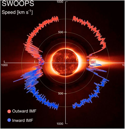
FIGURE 1. The solar wind speed distribution during the sunspot minimum condition (McComas et al. (2013).
Figure 1 shows that the speed is remarkably uniform with a speed of about 750 km/s over the whole latitude range between 20° and 80°. In this paper, this remarkable uniform part of the solar wind is called the Uniform flow (UF flow) in this paper. This uniform flow is cut off below the latitude of 20°. In this gap, the equatorial streamer takes its place. Since the observation was made when the solar activity was the lowest, the magnetic equator and the ecliptic equator almost coincide; see the tilt angle of the heliospheric current sheet [HCS] in Figure 2 and also Figure 3.
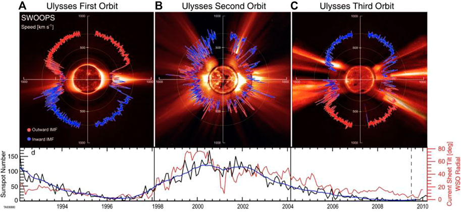
FIGURE 2. The latitudinal solar wind speed distribution: from the left during the minimum solar activity. (A) is same as Figure 1, (B) a high activity and (C) a weak activity; the Figure shows also the sunspot number and inclination of the heliospheric current sheet (McComas et al., 2013).
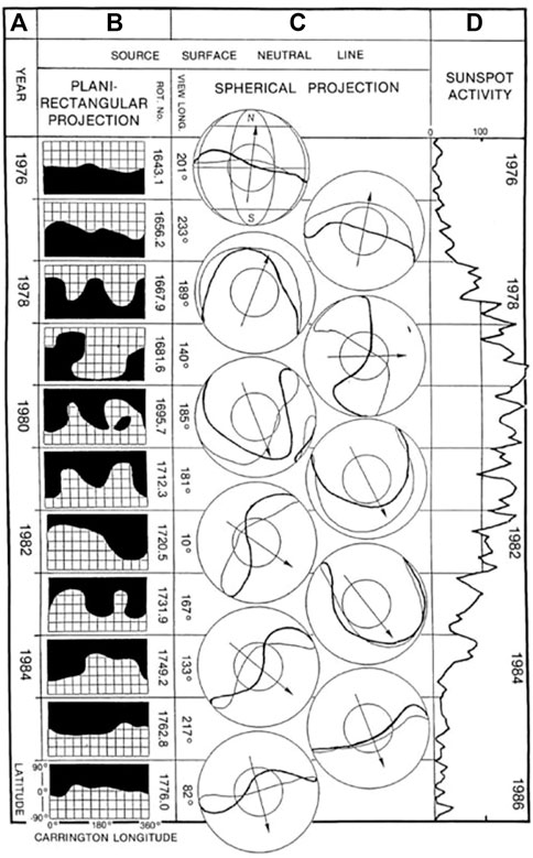
FIGURE 3. From the left: The neutral line dividing the positive and negative magnetic hemispheres on the source surface of the Carrington (2-D) map (WSO); Middle, the magnetic equator on the source surface (a 3-D format), together with the equivalent dipole axis based on the magnetic equator. Right; the sunspot number; Saito et al. (1989).
The basic distribution (Figure 1) may be graphically represented on the Carrington map [Latitude-longitude (27 days)] without the equatorial streamer.
In this map, one can consider that the Earth scans the map from left to right during one solar rotation. In this situation, since the Earth is located within the gap, it is not possible to observe the UF flow of 750 km/s; the change of ecliptic latitude of ±7° is partially responsible for higher speeds during equinox months; this change of the Earth’s location causes the equinox maximum of auroral activities.
Figure 2 shows the solar wind distribution during active periods of the Sun, including Figure 1 as Figure 2A; McComas et al. (2013). In order to study the wind speed distribution during active periods, it is necessary to know how the magnetic equator varies during the sunspot cycle.
The Wilcox Solar Observatory (WSO) publishes the neutral line on the source surface (a spherical surface of three solar raii) and presents it on the Carrington map. During active periods, it is often difficult to uniquely determine the magnetic equator on the phosphoric and also the source surface, so that they call it the neutral line, in stead of the magnetic equator; the neutral line in the Carrington map shows roughly the dividing line between the northern and southern magnetic hemispheres on the source surface. In this paper, however, their neutral line is called the magnetic equator.
Based on the WSO magnetic equator, (Hoeksema, 1984); Saito et al. (1989) presented the magnetic equator thus determined in a 3-D format for the sunspot cycle 21, which is shown in Figure 3; they determined also the equivalent dipole axis based on the magnetic equator thus determined. They examined also that the neutral line for the cycle 22 and 23 and found it similar to the cycle 21, so that the pattern in Figure 3 is the general trend. However, this presentation during a very high active period is obviously tentative, because of complex distribution of sunspots. Many studies related to the magnetic equator on the source surface are summarized by Akasofu et al. (2005).
The magnetic equator thus determined is close to the ecliptic equator during the beginning and the end of the solar cycle, but deviates from the ecliptic equator considerably during active periods. This trend is also seen as the rotation of the equivalent dipole axis by 180° during one sunspot cycle; see also the tilt angle HCS in Figure 2 (bottom).
The magnetic equator thus determined can be represented approximately by a sinusoidal curve on the Carrington map on the source surface, except extremely active periods. Figure 4 compares the magnetic equator of CR 1720 in 1982 with a pure sine wave case. It can be seen that the magnetic equator of CR 1720 (soon after the peak period, Figure 3) can approximately be represented by a quasi-sinusoidal curve on the Carrington map.
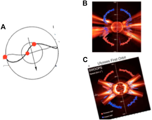
FIGURE 4. (A) The magnetic equator on the spherical source surface during a weakly disturbed condition (near the end of the cycle in this case); it is taken from Figure 3); the dots show the assumed location of equatorial streams. (B) The observed distribution (Figure 2C). (C) The constructed distribution of (B).
We demonstrate here that the basic speed distribution pattern represented by Figure 1 (same as Figure 2A) may be present throughout the solar cycle, and that Figure 2C (a low sunspot number period) and Figure 2B (a very high sunspot number) can be reproduced approximately by rotating counterclockwise Figure 1 (same as Figure 2A) according to the rotation of the magnetic equator and the equivalent dipole axis during the solar cycle.
(a) Weak activities
The magnetic equator deviates a little during the beginning and later periods of the cycle as shown in Figure 3. For a weakly active period of the cycle, Figure 1 is rotated about 20° counterclockwise and added the equatorial streamer at three positions along the magnetic equator (three red dots in Figure 4A) and by rotating the Sun once (by considering that the Ulysses observation took at least one rotation period (the observed distribution is not an instant scan along a single meridian line). Note also that the equatorial streamer may be absent on one side in Figure 1, indicating that the equatorial streamer is perhaps intermittently present along the magnetic equator.
Figure 4C thus constructed may be compared with the observed one (Figure 4B, reproduced from Figure 2C). One can see some resemblance between them. In particular, the UF flow can be seen over a wide latitude range in higher latitudes, and the wider gap is replaced by the streamers.
(ii) Active periods
The magnetic equator deviates considerably from the ecliptic equator during active periods, as shown in Figure 3. We choose the magnetic equator of CR 1720 shown in Figure 3 [or Figure 5 (left)] for the reproduction. Figure 1 is rotated counterclockwise by about 70° by adding the four equatorial streamers at the locations along the magnetic equator (red dots in Figure 6A); further, the Sun is rotated once. The results are shown in Figure 6C, which may be compared with the observed case of Figure 6B (the same as Figure 2B).
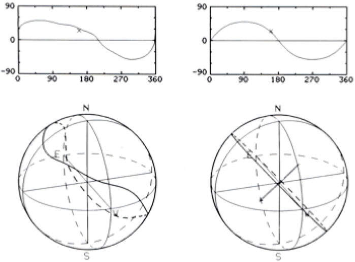
FIGURE 5. Left: Year, an example of the magnetic equator on the Carrington map and on the spherical source surface of CR 1720 shown in Figure 3 (but is rotated by 180° for the comparison). Right: A simple sine wave case; it shows also the equivalent dipole axis.
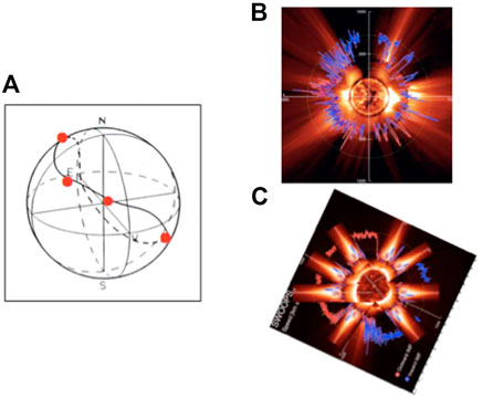
FIGURE 6. (A) The magnetic equator on the spherical source surface (CR 1720); dots show the assumed location of the equatorial streamers. (B) The observed distribution (Figure 2B). (C) The constructed distribution by rotating the sun once.
Comparing observed one (Figure 6B) and the constructed one (Figure 6C), one can see:
(i) The observed equatorial streamer is present at 70° in latitude. This location of the equatorial streamer is difficult to explain, unless the magnetic equator is located at the latitude of 70° as shown in Figure 6A (even if other streamers are present).
(ii) There are a few small parts of the UF flow in the mid-latitude. Thus, if the distribution during active periods is entirely different from the lowest solar condition (Figure 1), parts of the UF flow should not appear there. Thus, there is an indication that the distribution of Figure 1 is present even during some active periods, but it is difficult to recognize because of the distorted magnetic equator.
(iii) The observed equatorial streamer appears at a few more locations than Figure 6C.
(iv) The UF flow in the polar cap region is clearly present.
(v) There is not much UF flow at the locations where the streamers are present.
From these results, it is possible to consider that the speed distribution in Figure 1 (the UF flow with the equatorial streamer) is present even during active periods, but is obscured by the rotated magnetic equator and the equatorial streamers.
Based on the above findings, we modify the Carrington map in Figure 7 and construct a new one for fairly active periods in Figure 8, in which the magnetic equator is approximately representative by a sinusoidal curve of amplitude of 45° by considering an average active period; the width of the gap region is left as the same in Figure 7 for simplicity.
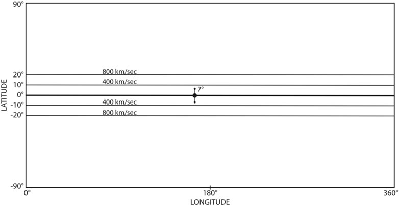
FIGURE 7. The speed distribution of the solar wind during the solar minimum period in the Carrington map. This is an approximate graphic representation of Figure 1, except the equatorial streamer. The Earth’s location is projected on the ecliptic plane.
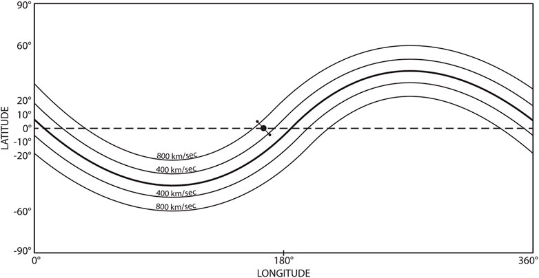
FIGURE 8. The wind speed distribution for an average active period on the Carrington map, by making the magnetic equator quasi-sinusoidal. The gap may be wider during active periods.
As the Earth scans the ecliptic equator from the left to right in the Carrington map, the Earth observes two long periods of the UF flow (750 km/s) and two lowest speed (350 km/s) between. These features are clearly observed particularly during the declining period of the sunspot cycle. Figure 9 showed such an example of the two peak periods and two minimum periods during one rotation period. This trend continued more than a year in 1974; see Figure 10.
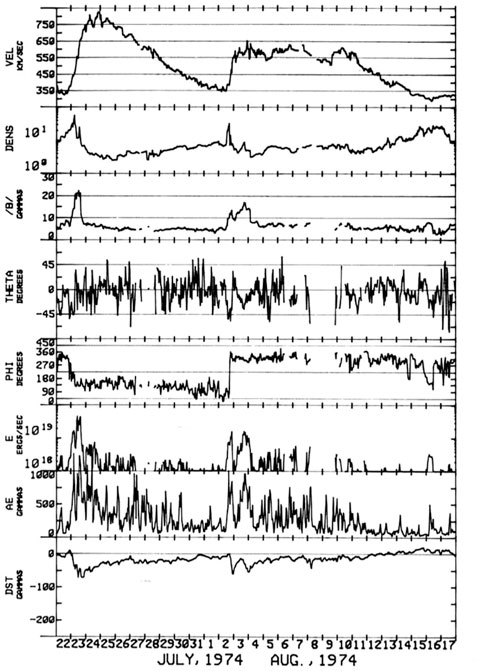
FIGURE 9. A typical example of solar wind observations in 1974. From the top, the solar wind speed, density, IMF magnitude B, IMF angles THETA and PHI, the solar wind-magnetosphere dynamo power ε (see Akasofu et al. (1988)), and geomagnetic indices AE and Dst.
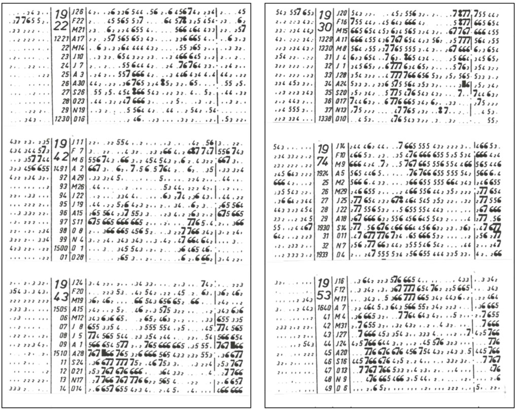
FIGURE 10. The C9 index during each Carrington day. From the left, the sunspot number index, Carrington number, year/beginning date, the C9 index (a part of the next cycle is repeated in the last part in order to see the two high speed periods).
The quasi-sinusoidal curve can also be inferred from the C9 geomagnetic index. The C9 index is a daily geomagnetic index and thus can be considered a smoothed version of the AE index as one can see in Figure 9 (except perhaps during major magnetic storms), so that it can be used to infer the general trend of solar wind speed variations. In fact, it has been available from about 1930 without interruption; for the C9 index, see Akasofu and Chapman (1972)).
Figure 10 shows the C9 index for several years. One can see two high geomagnetic activities lasting and two very low activities during 27 days for many months, corresponding the quasi-sinusoidal curve corresponding to Figure 8, namely, two UF flows, together with a very low speed between. Thus, from the C9 index we can infer the quasi-sinusoidal curve on the Carrington map; in some cases, one is weaker than the other, suggesting a distorted quasi-sinusoidal curve of Figure 8 or Figure 9. There are a large number study on the relationship between the solar wind and geomagnetic of storms. Most recently, Gerontidou et al. (2021) worked on this problem.
Figure 9 case can also be recognized in Figure 10 (Carrington Rotation 1928; July 22- August 17), indicating the usefulness of the C9 index in a study of the general trend of the solar wind speed from about 1930. Obviously. A sinusoidal magnetic equator is a simplest case. The magnetic equator takes more complex shapes during active periods.
Note thatjn one of the high speed flows comes from the northern hemisphere and the other from the southern hemisphere, as one can see in the PHI angle switch in Figure 9.
However, during the period of 1979–1980, it is known that the solar wind speed was abnormally low, only 350 km/s (NASA OMNI 50-day average solar wind data). During this period, there were hardly recognizable intense geomagnetic storms (C9 = 9), in spite of the fact that the sunspot number was very large, as can be seen in Figure 11 (right). The C9 index was generally small during this period (except a few Carrington days at the beginning of 1979), indicating also that the solar wind speed was also low.
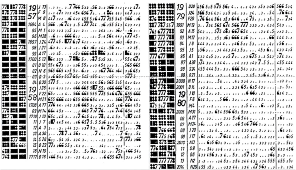
FIGURE 11. The C9 index during very active periods of the sun. The format is the same as that of this Figure. Left: In the middle period, two recurrent geomagnetic storms occurred, indicating that the quasi-sinusoidal curve was present. Right: There were hardly any intense geomagnetic storms during the later part of 1979 and 1980, suggesting also a low speed flow.
On the other hand, during the period of 1957–1958 (the IGY period) of Figure 11 (left), there was two recurrent geomagnetic storms; an active sunspot group can cause recurrent geomagnetic storms, but last at most three solar rotation periods, not 8 rotation periods. Thus, it shows that the quasi-sinusoidal curve survived even during a high sunspot activity period; In Figure 2B, we can recognize the UF flow, but there is no clear UF flow in the location where the streamers are present.
Based on Figures 2B, 11, we interpret thus that the very low speed during a very active period is due to the fact that the solar wind generation mechanism producing the UF flow in Figure 1 is disturbed by the equatorial streamer and sunspot associate helmet streamers and others; for the helmet streamers, see Linker et al. (2001) and Guo and Wu (1998). On the other hand, it seems that equatorial streamer and helmet streamers associated with sunspots may not be able to produce a high speed UF flow (750 km/s); this is also based on Figure 2B in which there is no clear UF flow where the equatorial streamer is present. This interpretation of the solar wind speed seems to be more reasonable than supposing an entirely different processes during very active periods.
These results provide hints on the long-held problem:
It has been the long-time problem why coronal holes can produce a very high speed flow or “stream” (750–800 km/s), in spite of the fact that there is not any particular activity there (no generally acceptable theory either), even if they are open regions; Cranmer (2009).
It is likely that the high speed flow or “stream” may be identified as the two UF flow resulting from the quasi-sinusoidal curve, rather than from coronal hole. The fact that two UF flow and two lowest flow exist in one solar rotation period are present supports this suggestion. This is particularly the case, because there is no activity to suggest a high speed flow; open field conditions Rotter et al. (2012) would not help without some activities.
Thus, it is suggested that the flow pattern represented in Figure 1 is actually the flow driven by the basic solar wind driving process itself.
Another point to examine is the fact that the solar wind speed was unusually low during very active sunspot periods. It was only 350 km/s for a long period in 1980. We suggest that the low speed (350 km/s) during the periods of very high spot numbers is due to the fact that the solar wind generation mechanism is disturbed by equatorial streamers and other solar activities. Parker (1991) suggested that heating the corona by Alfven waves and turbulence at a distance of 10 solar radii drives the solar wind; Lee and Akasofu (2021) suggested that a heliosphric-scale (J x B) force resulting from the solar unipolar induction current at a distance of about 10 solar radii is a part of the driving force of the solar wind. Thus, one possibility is that equatorial streamer could disrupt such a suggested origin at 10 solar radii (as shown in Figure 2B, in which there is no clear UF flow where the equatorial streamers are present). On the other hand, the streamers may not be able to produce the UF flow.
The present study suggests that the UF flow (Figure 1) observed by the Ulysses during the lowest sunspot represents the solar wind pattern driven by the basic solar wind generation process itself, instead of considering high speed flows from the open regions or from the polar coronal hole.
An extensive review by Viall and Borovsky (2020) showed that there is no generally acceptable theory of the driving process of the solar wind. It is hoped that the study presented here is useful in the search of the driving mechanism of the solar wind. Thus, our future work is to search for the driving process, which can reproduce Figure 1.
The original contributions presented in the study are included in the article/Supplementary Material, further inquiries can be directed to the corresponding author.
Data collaboratively analyzed by both authors. S-IA wrote the document with contributions from L-CL.
SEISA—funds received for publication fees G0759, 360903-66918.
We would like thank both Dr. K. Hakamada and Dr. T. Saito for their work on the solar magneticfield. Without their work, it is not possible to complete the results reported in our paper. No new data set is used in this paper.
The authors declare that the research was conducted in the absence of any commercial or financial relationships that could be construed as a potential conflict of interest.
All claims expressed in this article are solely those of the authors and do not necessarily represent those of their affiliated organizations, or those of the publisher, the editors and the reviewers. Any product that may be evaluated in this article, or claim that may be made by its manufacturer, is not guaranteed or endorsed by the publisher.
Akasofu, S.-I., and Chapman, S. (1972). Solar terrestrial relationship. Oxford, UK: Oxford University Press.
Akasofu, S.-I., Olmstead, C., Saito, T., and Oki, T. (1988). Quantitative forecasting of the 27-day recurrent magnetic activity. Planet. Space Sci. 36, 1133–1147. doi:10.1016/0032-0633(88)90068-2
Akasofu, S.-I., Watanabe, H., and Saito, T. (2005). A new morphology of solar activity and recurrent geomagnetic disturbances: The late-declining phase of the sunspot cycle. Space Sci. Rev. 120, 27–65. doi:10.1007/s11214-005-8052-3
Akasofu, S. I. (2023). A new understanding of why the aurora has explosive characteristics. Mon. Not. Roy. Astron. 518, 3286–3300. doi:10.1093/mnras/stac3187
Cranmer, S. R. (2009). Coronal holes, living rev. Solar Phys.,6, 3. Speed Dur. Minim. between Cycles 23 24 Sol. phys 274, 195–217. https://www.livingrviews.org/lrsp-2009-3.
Gerontidou, M., Mavromichalaki, H., and Daglis, T. (2018). High-speed solar wind streams and geomagnetic storms during solar cycle 24. Sol. Phys. 293 (9)–131. doi:10.1007/s11207-018-1348-8
Guo, W. P., and Wu, S. T. (1998). A magnetohydrodynamic description of coronal helmet streamers containing cavity. ApJ. 494, 419–429.
Hoeksema, J. T. (1984). “Structure and evolution of the large scale solar and heliospheric magnetic fields,”. Ph.D Thesis (Cambridge, MS, USA: Harvard University).
Kumar, A., and Badruddin, 2002. Study of the evolution of geomagnetic disturbances during the passage of high coronal holes in the solar cycles 2009-2018. Astrophysics and Space Sci., 366 (2) art. No. 21.
Lee, L. C., and Akasofu, S. I. (2021). On the causes of the solar wind: Part 1. Unipolar solar induction currents. J. Geophys. Space Phys. 126, 1–8. doi:10.1029/2021JA029358
Linker, J. A., Lionell, R., and Mikic, Z. (2001). Magnetodydrodynamic modeling of prpminence formation within a helmet streamer. J. Geophys. Res. 106, 23165–25175.
McComas, D. J., Angold, N., Eliott, H. A., Livadiotis, G., Schwadron, N. A., et al. (2013). Weakest solar wind of the space age and the current "mini" solar maximum. ApJ 779 (10), 2. doi:10.1088/0004-637x/779/1/2
Parker, E. N. (1991). The phase mixing of Alfven waves, coordinated modes and coronal heating. ApJ 376, 355–363. doi:10.1086/170285
Rotter, T., Verrong, A. M., Vrsnk, B., and Vrsnak, B. (2012). Relation between coronal hole areas on the sun and the solar wind parameters at 1 AU. Sol. Phys. 281, 793–813. doi:10.1007/s11207-012-0101-y
Saito, T., Oki, T., Akasofu, S.-I., and Olmsted, C. (1989). The sunspot cycle variations of the neutral line on the source surface. J. Geophys. Res. 94, 5453–5455. doi:10.1029/ja094ia05p05453
Schwenn, R. (2006). Space weather: The solar perspective. Living Rev. Sol. Phys. 3, 2. doi:10.12942/lrsp-2006-2
Sheeley, N. R., Wang, Y.-M., Hawley, S. H., Brueckner, G. E., Dere, K. P., Howard, R. A., et al. (1997). Measurements of flow speeds in the corona between 2 and 30 R☉. ApJ. 484, 472.
Shugai,, , Yu., S., Veselovsky, I. S., and Trichtchenko, L. D. (2009). Studying correlations between the coronal hole area, solar wind velocity, and local magnetic indices in Canadian region during the decline phase of cycle 23. Geomagn. Aeron. 49, 415–424.
Verscharen, D., KristopherKlein, K. G., and Maruca, B. A. (2019). The multi-scale nature of the solar wind. Living Rev. Sol. Phys. 165. doi:10.1007/s1116-018-0021-0
Viall, N. M., and Borovsky, J. E. (2020). Nine outstanding questions of solar wind physics. J. Geophys. Res. Space Phys. 125. doi:10.1029/2018JA026005
Wang, Y. M. (2012). Semiempirical models of the slow and fast solar wind. Space Sci. Rev. 172, 123–143. doi:10.1007/s11214-010-9733-0
Keywords: solar wind, Ulysses, solar cycle, geomagnetic storm, solar magnetic field
Citation: Akasofu S-I and Lee L-C (2023) The basic solar wind speed distribution and its sunspot cycle variations. Front. Astron. Space Sci. 10:1129596. doi: 10.3389/fspas.2023.1129596
Received: 22 December 2022; Accepted: 27 March 2023;
Published: 13 April 2023.
Edited by:
Joseph E. Borovsky, Space Science Institute, United StatesReviewed by:
Dhani Herdiwijaya, Bandung Institute of Technology, IndonesiaCopyright © 2023 Akasofu and Lee. This is an open-access article distributed under the terms of the Creative Commons Attribution License (CC BY). The use, distribution or reproduction in other forums is permitted, provided the original author(s) and the copyright owner(s) are credited and that the original publication in this journal is cited, in accordance with accepted academic practice. No use, distribution or reproduction is permitted which does not comply with these terms.
*Correspondence: Syun-Ichi Akasofu, c2FrYXNvZnVAYWxhc2thLmVkdQ==
Disclaimer: All claims expressed in this article are solely those of the authors and do not necessarily represent those of their affiliated organizations, or those of the publisher, the editors and the reviewers. Any product that may be evaluated in this article or claim that may be made by its manufacturer is not guaranteed or endorsed by the publisher.
Research integrity at Frontiers
Learn more about the work of our research integrity team to safeguard the quality of each article we publish.