The upward propagating ionospheric hiss waves during the seismic time observed by the China seismo-electromagnetic satellite

The ionospheric hiss wave is a broadband incoherent and structureless electromagnetic emission. They appear in a relatively narrower frequency range between −0.1 and 1.5 kHz. However, according to previous observations, abnormal electromagnetic emissions during seismic activities also preferentially appear in the same frequency range of ionospheric hiss. This work studies the propagation features of the ionospheric hiss during seismic time based on the observations from the CSES (China Seismo-Electromagnetic Satellite). The wave vector analysis shows that during seismic activities, except for the downward propagating ionospheric hiss which is a common phenomenon in the ionosphere, there are upward propagating emissions mixed with the downward propagating ionospheric hiss. We made a statistical analysis of the shallow strong earthquakes (M ≥ 6.0, depth below 30 km) that occurred in mainland China from 2019 to 2022. We selected the ionospheric hiss events recorded by orbits passing over the epicenters within a time window (the 1-month prior to and 1-week after the main shock). We found that although most of the events are the typical downward propagating ionospheric hiss waves, however, there are certain events mixed with the upward propagating emissions. The statistical distribution analysis of wave propagation parameters shows that the major part of wave normal angles vary from 40 to 60, the azimuthal angles predominately attain below 40, and the ellipticity shows a more complicated feature varying around ± 0.5, and the planarity values predominate at values between 0.6 and 1. The frequency band of the upward propagating ionospheric hiss mostly varies between 300 Hz and 800 Hz. To further study the behavior of such upward propagating ionospheric hiss wave during the seismic time, we compared the wave activities under non-seismic activity and quiet space weather conditions, and the results confirm that the occurrence rate of the upward propagating emissions under quiet conditions is far less than that in the seismic time. We suggest that there is a link between the upward propagating ionospheric hiss and the seismic activity, but the physical reason behind it still remains a puzzle to us.

1 Introduction

The hiss wave is a broadband structureless electromagnetic emission that are preferentially observed in the high electron density geospace. According to their locations, there are two main types of hiss waves identified by the previous studies: one is the plasmaspheric hiss which is mostly observed inside the plasmasphere region (Thorne et al., 1973); the other is the ionospheric hiss (Chen et al., 2017) which just appears in the ionosphere in the lower altitude. The former predominately appears in a frequency range from −0.1 to 3 kHz, while the latter appears in a relatively narrower frequency range between −0.1 and 1.5 kHz (Xia et al., 2020; Zhima et al., 2017). Both observations and ray-tracing simulations suggest that the plasmaspheric hiss (Chen et al., 2017; Zhima et al., 2017) or the lower band whislter-mode chorus waves (Santolík et al., 2006) can penerate the plasmapuase and enter into ionosphere in the high latitude, finally can excite the ionoshperic hiss under certain conditions. Zhima et al. (2017) found evidence of a close link between the plasmaspheric and ionospheric hiss waves from conjugate observations based on DEMETER (Detection of Electromagnetic Emissions Transmitted from Earthquake Regions) flying inside the ionosphere and THEMIS (Time History of Events and Macroscale Interactions during Substorms) which is located inside the inner magnetosphere.

In recent decades, thanks to the successful operation of electromagnetism satellites in low earth orbit (LEO) space, the ionospheric hiss gets well recorded. The DEMETER is the first electromagnetism satellite with a scientific objective of monitoring earthquake activities from the lithosphere, it was in orbit from −2004 to 2010 at altitudes from −710 to 660 km (Parrot et al., 2006), brought us valuable observations on the electromagnetic field. The second electromagnetism satellite for earthquake monitoring is the CSES (China-Seimo-Electromagnetic Satellite) which was launched in February 2018 and is currently in operation at an altitude of −507 km (Shen et al., 2018). The observations both from DEMETER and CSES demonstrate that the ionospheric hiss waves most commonly distribute along the local proton cyclotron frequency, showing clear upper and lower cutoff effects (Wang et al., 2022). (Chen et al., 2017) further identified that there are two types of ionospheric hiss: Type I and Type II. Type I is characterized by vertically downward propagation and broadband spectral property at high latitude, while Type II is featured with equatorward propagation and a narrower frequency bandwidth closely along the local proton cyclotron in the mid-low latitude. Theoretical analysis futher suggests that Type II emission is most likely generated by the magnetospheric whistler emission that accesses the high latitude ionosphere region, and Type I emission is probably formed by the wave-trapping effect due to the local ions’ cutoff frequency and gradient of plasma density (Chen et al., 2017).

Interestingly, according to previous studies, we found that most of the abnormal electromagnetic emissions during major earthquakes (EQs) also preferentially appear in the same frequency range of ionospheric hiss. For example, Larkina et al. (1989) found that the abnormal ELF/VLF emissions before strong EQs appeared in a frequency range from 0.1–1.6 kHz based on the observations of Intercomos-19 and Aureol-3 satellites; Serebryakova et al. (1992) found the abnormal emissions below 450 Hz before seismic activity by using observations from COSMOS-1809 and AUREOL-3 satellites [M; Parrot, 1994]. suggested that the wave intensity close to the epicenter predominantly increased at the frequency below 800 Hz based on a statistical analysis for 325 EQs (Magnitude ≥5) from AUREOL 3 satellite. Błeçki et al. (2010) reported the existence of strong emissions in the frequency range below 800 Hz within 1 week before the disastrous 2008 Wenchuan Mw 8.0 EQ based on the observations of DEMETER satellite. Zhima et al. (2020a) reported that the abnormal EM emissions (–300–800 Hz) were propagating upward to outer space from the Earth direction about 10 to 3 days period before the main shock of the Mw 7.8 northern Sumatra earthquake (6 April 2010). Nemec et al. (2009) reported that the wave intensity around 1.7 kHz appeared a very small but statistically significant decrease about 0–4 h before EQs based on a stastical analysis of 3.5-year observations from the DEMETER; Chmyrev et al. (1997) found a small-scale plasma inhomogeneities and simultaneous excitation of abnormal EM waves at the ELF frequency band (e.g., 140 Hz and 450 Hz) over the seismic zones from the Cosmos-1809 satellite.

The mixture of different sources of emissions in the same frequency band brings us a challenge to correctly identify or extract the real seismic precursors. So this work is motivated to study the relationship between ionosphere hiss emissions during seismic occurrences.

2 Dataset and method

We utilized the observations from the China Seimo-Electromagnetic Satellite (CSES) which is the first electromagnetism probe of China’s Zhangheng mission. The Zhangheng mission is aimed to detect the geophysical field by launching both the electromagnetism and gravity micro-satellite in the Low Earth Orbit in the future decades. The Zhangheng misssion is named after the ancient Chinese scientist Zhangheng who invented the seismo-scope in the second century.

The CSES is aimed to monitor the seismic activities from space (Shen et al., 2018; Zhima et al., 2022), and it was launched in 2018 on a circular Sun-synchronous orbit at an altitude of about 507 km in the upper ionosphere, with an inclination of 97.4. The CSES flies 15.2 orbits around the global Earth per day at the local time around 02:00 a.m. (nightside) and 2:00 p.m. (dayside), respectively. It has a 5-day revisiting period for the same area. Until now, CSES has been steadily operating in orbit for over 5 years. Its identical successor satellite CSES 02 will be launched in the same orbit space around 2024. The CSES measures the total geomagnetic field, the electromagnetic field and waves, the energetic particles, and the ionospheric parameters in the region within the latitude of ± 65. In this study, we mainly used the total magnetic field and the electromagnetic field detections from CSES, and the involved payloads are briefly introduced as follows.

The geomagnetic field is detected by the high-precision magnetometer (HPM), which consists of two tri-axial fluxgate sensors (FGMs) (Zhou et al., 2018) and one coupled dark-state magnetometer (CDSM) (Pollinger et al., 2018). The FGMs provide the magnetic field vector data in the frequency from DC (Direct Current) to 15 Hz, and CDSM serves as a reference to FGM by providing the scalar value of the total magnetic field. CSES carries a tri-axial search coil magnetometer (SCM) to detect the variant magnetic field with three detection frequency bands: ULF (Ultra-Low-Frequency, 10–200 Hz), ELF (Extremely-Low-Frequency, 200 Hz −2.2 kHz), VLF (Very-Low-Frequency, 1.8 kHz–20 kHz) (Cao et al., 2018). The electric field detector (EFD) onboard CSES can provide the spatial electric field with the four detection frequency bands: ULF (DC -16 Hz), ELF (6 Hz—2.2 kHz), VLF (1.8 kHz–20 kHz), HF (High-frequency, 18 kHz—3.5 MHz) (Huang et al., 2018). CSES operates with two working modes: survey (lower sampling rates along the whole orbit trajectory) and burst mode (a higher sampling rate but only triggered above the global main seismic belts). In the ELF band both SCM and EFD can can continuously provide six-component waveform data along the whole trajectory in the survey mode, allowing us to compute the wave propagation parameters at any time of interest.

So in this study, we adopted the Singular Value Decomposition (SVD) method (Santolik and Gurnett, 2003) to determine the propagation direction of the ionospheric hiss waves. The SVD method has been widely used in space electromagnetic waves propagation (Chen et al., 2017; Parrot et al., 2016; Wei et al., 2007; Zhima et al., 2020b), through which, the propagation directions of EM emissions can be determined. According to our knowledge, the downward ionospheric hiss waves (coming above the orbit space and propagating downward Earth direction) are most likely linked to the plasmaspheric hiss in the plasmasphere (Chen et al., 2017) or the chorus waves in the inner magnetosphere (Santolík et al., 2006; Tsurutani et al., 2012); and the upward ones (coming below of the orbit space and propagating upward the outer space from the Earth direction) are possibly originated by the lightning activities (Zhima et al., 2017) in the atmosphere or the earthquake (Zhima et al., 2020a) in the Lithosphere.

The wave propagation parameters such as the wave vector, and the wave polar and azimuthal angles are defined under a Magnetic Field Aligned Coordinate (MFAC) system (Santolik and Gurnett, 2003). As shown in Figure 1, we define the Z-axis points along with the background magnetic field B₀, the Y-axis is directed along the cross product of the Z-axis and the position vector of the satellite (so that the +Y-axis is nominally eastward at the equator), and the X-axis completes a right-handed system (Hu et al., 2023) under the MFAC system. According to the SVD algorithm, we can use two angles to define the relationship between the wave vector k and the background magnetic field B₀, one is the polar angle θ_k, and the other is the azimuthal angle φ_k. We can determine whether the wave vector is parallel or perpendicular to the ambient magnetic field B₀ by the wave normal angles θ_k (0 – 90); and determine the wave propagates towards the decreasing L shell direction in the meridian plane by the values of φk (±180°), Figure 4 or propates to the local magnetic meridian plane (φk = 90°) (Hu et al., 2023).

FIGURE 1

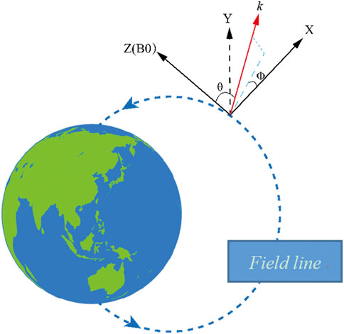
FIGURE 1. The definition of MFAC coordinate [revised based on of Hu et al. (2020)].

So firstly, we used the three components of the total magnetic field vector data recorded by HPM onboard to build the MFAC system. Then, we separately converted the electric field vector (Ex, Ey, Ez) and magnetic field vector (Bx, By, Bz) from the geographic coordinate system (GEO) which is a standard data product published by the CSES scientific center, into the MFAC system. The waveform data under the GEO and MFAC is plotted in Figure 2. After that, we computed the wave propagation parameters by the SVD algorithm based on MFAC.

FIGURE 2

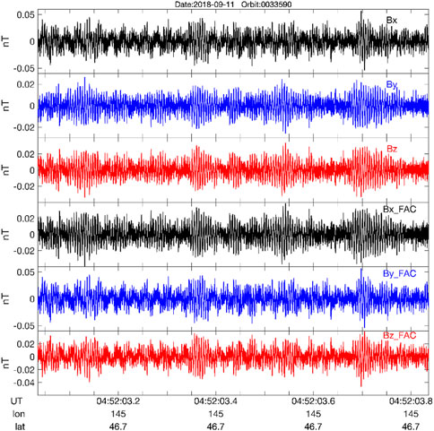
FIGURE 2. An example of waveform data rotated from the GEO (Bx, By, Bz) and MFAC system (Bx_FAC, By_FAC, Bz_FAC).

3 Analysis

The ionospheric hiss waves, as shown in Figure 1 by Chen et al. (2017), Figure 2 by Hu et al. (2020), or Figure 1 by Wang et al. (2022), exhibit intense structureless features along the local proton cyclotron frequency. This kind of EM emissions is recorded by almost every orbit of DEMETER (altitudes from 660 to 710 km) and CSES (altitudes −507 km) satellites in the upper ionosphere, and the wave intensity and distribution are primarily dependent on disturbed space weather conditions. Xia et al. (2020) statistically examined DEMETER’s 6-year observations on ionospheric hiss waves and described their dependence on local time, location, season, and geomagnetic activity; Wang et al. (2022) statistically studied the ionospheric hiss based on CSES’s observations, and found that the ionospheric hiss along the local proton cyclotron frequency primarily occur in the mid-high latitude (–20°–55°) in the dayside ionosphere, and their bandwidth decreases with magnetic latitude, showing a clear lower cutoff frequency, but a relatively diffuse upper cutoff frequency.

The characteristics of wave properties and occurrence rates of the ionospheric hiss waves have been well described by previous studies (Wang et al., 2022; Xia et al., 2020). In this work, we focus on the ionospheric hiss waves which appear between the lower cut-off frequency and the local proton cyclotron frequency, as shown by red squares in Figure 3. Figure 3 is one example of this kind of wave event recorded on 09 June 2019. The magnetic field wave intensity presented by the power spectral density (PSD) values is given in Figures 3A,B shows the electric field wave intensity in a frequency range from 200 to 1000 Hz. The black dashed lines are the local proton cyclotron frequency (f_cp) which was computed by the total magnetic field data from HPM onboard CSES. Figure 3C shows the orbit trajectory. It is seen that there is a bulk of intense structureless hiss waves appearing at a frequency range roughly from 300–700 Hz (denoted by red squares in Figures 1A,B), their location is highlighted by the red thick bar in Figure 3C. It is noted that such wave structures in the frequency range from −300 to 700 Hz are quite common in CSES’s electromagnetic observations.

FIGURE 3

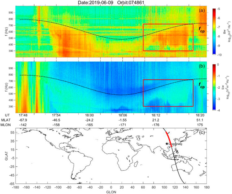
FIGURE 3. The ionospheric hiss wave recorded by CSES on 09 June 2019 (orbit No.074861).

Further, we computed the wave propagation parameters using the SVD method, as shown in Figure 4. Figures 4A,B show the PSD values of the magnetic and electric fields computed by waveform data in the ELF band. The points where the magnetic field PSDs are lower than certain values were removed to highlight the natural ionospheric hiss emissions. Figure 4C is the ellipticity value, representing the ratio of the axes of the polarization ellipse (−1: left-handed, 0: linear polarization, +1: right-handed circular polarization). It is seen that the waves show mixed polarization features, and the ones in the red square are dominated by the right-hand circular polarized in most areas.

FIGURE 4

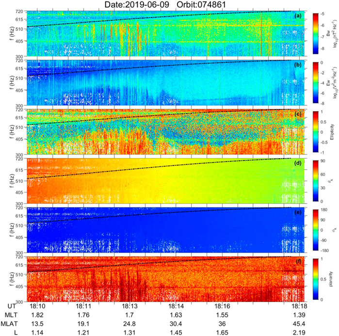
FIGURE 4. The wave propagation parameters computed by the SVD method for the observations of the red squares of Figure 3 From top to bottom: (A) the PSD values of the magnetic field; (B) the PSD values of the electric field; (C) the ellipticity; (D) the wave normal angle; (E) the azimuthal angle for the wave vector K; (F) the planarity. Data are displayed as a function of universal time (UT), magnetic local time (MLT), geomagnetic latitude (mlat), and L shell, respectively.

Figure 4D shows the variation of the wave-normal angles φ_k, which roughly range from 40 to −50. Thus it can be reasonably concluded that the waves are obliquely propagating. Figure 4E shows the azimuthal angle, φ_k, which attains a value of −180°. It is defined in the MFAC framework (Figure 1), a value of azimuthal φ_k = ±180° indicates the wave propagating towards the decreasing L shell direction in the meridian plane (i.e., toward the Earth direction). Thus, Figure 4 indicates that the waves propagate from somewhere above the satellite orbit to the Earth’s direction. The waves observed in Figure 4F exhibit a planarity value of − +1, indicating that the observed waves are propagating towards the spacecraft in the form of a plane wave. (0 is the value indicating a spherical propagation).

During the seismic activity time, we found that this kind of ionospheric hiss waves sometimes is mixed by the upward propagating emissions. For example, Figure 5 shows an event recorded about 26 days before the Ms 7.4 Maduo EQ which struck southwest China on 18 May 2021, with an epicenter location at Lat = 34.59, Long = 98.34°and with a depth of 17 km. Obviously, from Figure 5, it is hard to tell any difference from the event as shown in Figure 3. However, through the wave vector analysis, as shown in Figure 6, the differences between the wave propagation parameters can be identified.

FIGURE 5

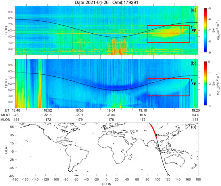
FIGURE 5. The ionospheric hiss recorded by CSES (No. 179291 on 26 April 2021) before the Maduo Ms 7.4 EQ occurred on 22 May 2021.

FIGURE 6

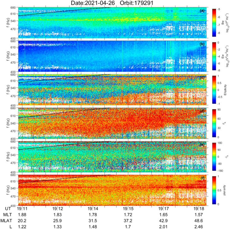
FIGURE 6. Same format as Figure 4, but for the wave propagation parameters of the waves in the red squares in Figure 5.

In Figure 6C, the ellipticity values show a mixed polarization feature, including right/left-handed and linear polarizations. In this event, the wave-normal angles φ_k in Figure 6D, predominated around 60 –90, meaning the waves almost perpendicularly propagate along the magnetic field line. Most importantly, Figure 6E shows that the azimuthal angle, φ_k is predominated by 0 (green color). In the MFAC framework, φ_k = ± 0 indicates that the waves are propagating towards the increasing L shell direction in the meridian plane. Figure 6F shows that the planarity of the waves varies mainly from 0.5 to + 1, implying that the waves are propagating as a plane wave towards the spacecraft.

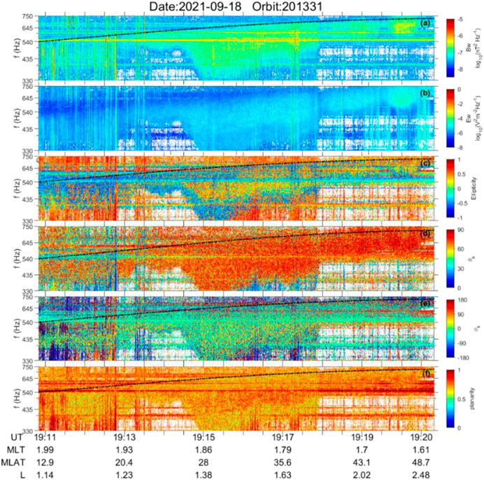
Figure 7 presents another event that occurred 2 days after the Luxian Ms 6.0 EQ which struck southwest China on 16 September 2021. It is clearly seen that Figure 7 exhibits similar wave properties as Figure 3. Figure 8 shows the wave propagation parameters. As the feature shown in Figure 6, the ellipticity values in Figure 8C show complicated features, with a mixture of the right/left-handed and linear polarizations. In this event, the wave-normal angles θ_k are large, most of them are 60–90. There is a large number of azimuthal angles φ_k remaining around 0 in Figure 8E, meaning there is an upward propagation direction. From Figure 8F, we can tell these emissions are almost a plane wave propagation feature.

FIGURE 7

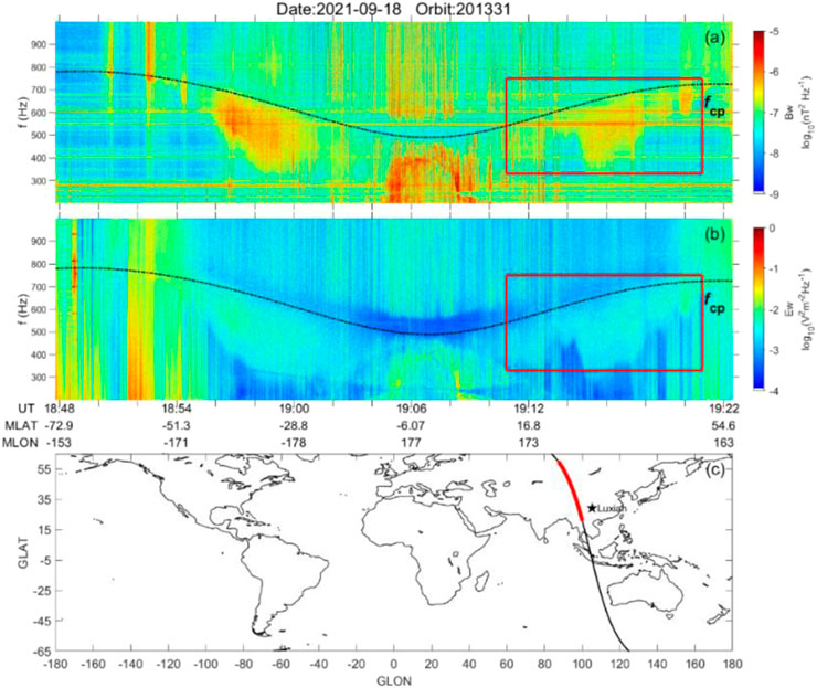
FIGURE 7. The ionospheric hiss appeared 2 days (No. 201331 on 18 September 2021) after the 2021 Luxian Ms 6.0 EQ (21 September 2021).

FIGURE 8

FIGURE 8. Similar to that of Figure 4, but for the waves in the red squares in Figure 7.

4 Discussion

To further understand the behavior of the ionospheric hiss waves during seismic activity time, we selected all the 14 shallow strong EQs (Depth: ≤30 km, Magnitude: ≥6) that occurred in mainland China from 2009 to 2022, as shown in Figure 9. The circles present the epicenter locations and magnitudes: the larger the size of the circles, the larger magnitudes of the earthquakes. The light-blue lines in Figure 9 represent the orbits of CSES, which repeat every 5 days to the same orbit trajectory. Detailed information about each EQ is listed in Table 1.

FIGURE 9

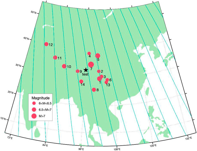
FIGURE 9. Strong shallow earthquakes (Depth: ≤30 km, Magnitude: ≥6) occurred in mainland China from 2019 to 2022. The circles denote the epicenter locations as well as the magnitudes of EQs (size of circles). The light-blue lines present the CSES’s orbit traces which regularly pass by over China with a recursive period of 5 days. The black star represents the test point of the wave activity under quiet conditions (see text).

TABLE 1

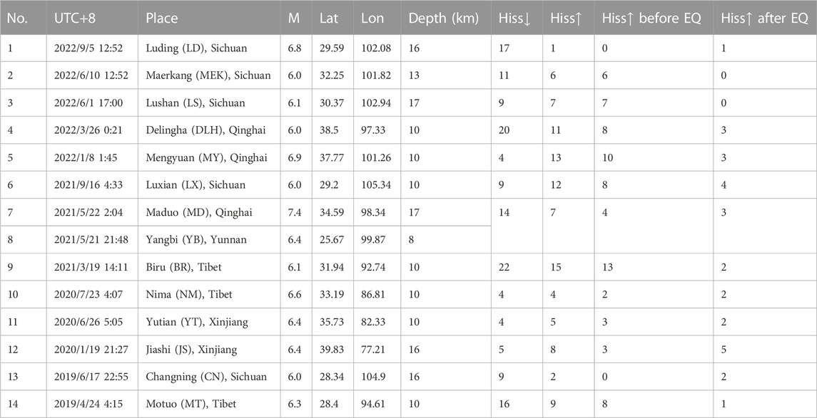
TABLE 1. The ionospheric hiss waves recorded by CSES during the seismic times in mainland China.

For each EQ, we checked the observations in a time window from 1 month before and 1-week after the mainshock, to search ionospheric hiss events (as shown in Section 3) from the orbits which pass over the epicenter areas. For simplicity of analysis, we just selected those well-recorded ionospheric hiss events as shown in Figure 3. Then, we further computed the wave propagation parameters for each event. The results for those 14 EQs are listed in Table 1.

For example, during the Ms 6.9 Menyuan EQ which struck Qinghai Province on 18 January 2022, we found four ionospheric hiss events dominated by the downward propagating emissions (denoted by hiss ↓ in Table 1), and 13 events mixed with the upward propagating emissions (denoted by Hiss↑ in Table 1). It is noted that due to the epicenters of Ms 7.4 Maduo (22 May 2021) and Ms 6.4 Yangbi (21 May 2022) are very close, so the ionospheric hiss events are counted together, in which we found 14 downward propagating events and 7 downward propagating events during these two EQs.

It is seen from Table 1 that there are some upward propagating ionospheric hiss events excited during the seismic time, although the downward propagating hiss wave events are more than the upward propagating ones. We further analyzed the distributions of wave propagation parameters for all the events in Table 1, as shown in Figure 10. It is seen that the majority of wave normal angles θ vary from 40 to 60, and the azimuthal angles φ predominately attain below 40. The ellipticity mainly varies around ± 0.5. The planarity predominates at values between 0.6 and 1.

FIGURE 10

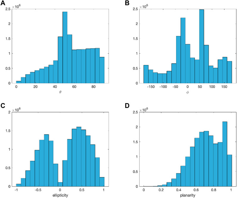
FIGURE 10. The statistical distribution of wave propagation parameters for those events mixed with the upward propagating emissions during the seismic time; (A) the wave normal angle θ, (B) the wave azimuthal angles φ, (C) the planarity, (D) epllipity.

Further, we examined the propagation parameters distributions along the frequency domain for all the upward propagating ionospheric hiss during the 14 EQs, as shown in Figure 11. As seen in Figure 11, there is a statistical feature of those upward propagating ionospheric hiss waves during the seismic time: the azimuthal angles mostly keep below 40 with a peak around 20 (Figure 11B) at a frequency band from 300 Hz towards 800 Hz, and the wave normal angles mainly peak at a narrower span from 40 to 50 at this frequency band (Figure 11A).

FIGURE 11

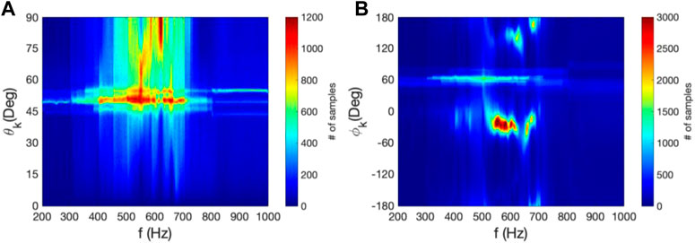
FIGURE 11. The distribution of wave propagation parameters along the frequency for those ionospheric events mixed with upward propagating emissions; (A) the wave normal angle θ, (B) azimuthal angles φ.

To further understand the behavior of such upward propagating ionospheric hiss waves during the seismic time, we compared the wave activities under quiet conditions: no strong shallow EQs (Depth: ≤30 km and Magnitude: ≥ 6) occurred under the quiet space weather condition (Dst index: ≥30 nT and Kp index: ≤3) within 1 month (30 days). We selected a test point (longitude: 96.3°E, Latitude: 32.5°N) as denoted by the black star in Figure 9. In total, we found four quiet periods over the test area (96.3 E± 10° and 32.5°N± 10°) from 2019 to 2022. Then we examined the ionospheric hiss events during the four time periods and computed their wave propagation parameters with the same methods, the results are given in Table 2. Comparing Table 1 and Table 2, it can be seen that the occurrence rate of the upward ionospheric hiss under quiet conditions is far less than that in the seismic time.

TABLE 2

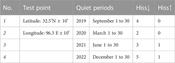
TABLE 2. The ionospheric hiss wave activity under quiet conditions over a test area.

Zhao et al. (2021) built an ELF wave propagation model to simulate the propagating process of waves from the lithosphere to the ionosphere, and results show that the wave power decreases with increasing frequency due to skin effect through an isotropic conductive medium. In other words, the higher frequency waves are more easily attenuated by the medium, leading to their propagation path being relatively short. By contraries, the lower frequency waves are less attenuated and more likely to propagate far into the ionosphere, however, the weaker radiation efficiency of the lower frequency waves confines their propagation extension. Additionally, the lower the depth, the lower frequency of waves that can be observed by satellite. The simulation from Zhao et al. (2021) suggests that the EM waves radiated from an EQ with a magnitude more than 6.0 can be recorded by CSES, but there exists a dominant frequency band for waves radiated from the epicenters with depths from 20 km to 10 km in the lithosphere. The dominant frequency is about 300 Hz for a source with a 10 km depth and the dominant frequency might be 100 Hz for a depth of 20 km.

It can be well understood from Figures 2, 3 by Zhao et al. (2021) that the wave power of the EM waves radiated by the EQs with a magnitude greater than 6.0 can propagate to high altitudes. At CSES’s orbit space, the wave power can sustain a higher level (–0–20 dB) at the frequency band from 20 Hz to 1000 Hz; and at a frequency higher than 1000 Hz, the wave power dramatically declines to below 0 dB. This study suggests that the upward propagating emission mostly appears at a frequency band from 300 Hz to 800 Hz. During the Mw 7.8 Northern Sumatra Earthquake in 2010, Zhima et al. (2020a) found similar upward propagating emissions at a frequency range from 300–800 Hz over the epicenter zone, at 10 and 6 days before the main shock. The possible existence of acoustic-gravity wave (AGW) was discussed by computing the potential energy variation of AGW using air temperature data and confirmed the link between the abnormal ELF emissions and the earthquake activity.

The physical process (Molchanov et al., 2004; Pullinets and Ouzounov, 2018; Sorokin et al., 2003) behind such upward propagating electromagnetic emissions is still a challenging scientific problem. By using a complex multidisciplinary approach, Pulinets and Ouzounov (2018) put forward the Lithosphere-Atmosphere-Ionosphere Coupling (LAIC) mechanism to interpret the physical processes of seismo-ionospheric phenomena associated with strong earthquakes. It is known that the radon or other types of gases (e.g., methane, helium, hydrogen, and carbon dioxide) in the lithospheric fault zone can leak from the lithosphere into the atmosphere, subsequently, those gases in the atmosphere can change the air conductivity resulting in a vertical electric current. The generation of local electric current can develop AGW instabilities as well as a horizontal inhomogeneity of ionospheric conductivity, finally generating the magnetic field-aligned currents, plasma irregularity, or the ULF/ELF emissions (Sorokin et al., 2001). It is necessary to interpate the mechanism through a multidisciplinary synergy (Ouzounov et al., 2018) by considering the simultaneous observations at different altitudes. The lithosphere-atmosphere-ionosphere system is a dynamic system, which is sensitive to various kinds of disturbances source (such as solar activities, geomagnetic storm, Lightning, human activity, etc.). However, the earthquake precusors are relatively weak and transient, can be submerged by other stronger perturbations. At present, we still lack reliable experimental evidences at different layers to interprate the phyiscal processing of earthquake precursors. Many of previous studies still require further experimental confirmation and objective statistical studies.

5 Conclusion

The ionospheric hiss waves display intense structureless features along the local proton cyclotron frequency. This kind of EM emissions is recorded by almost every orbit of CSES (altitudes −507 km) in the upper ionosphere. Their intensities and distribution extensions are primarily dependent on disturbed space weather conditions, and their bandwidth decreases with magnetic latitude, showing a clear lower cutoff frequency, but a relatively diffuse upper cutoff frequency. The statistical characteristics of wave properties and occurrence rates of the ionospheric hiss waves have been well described by previous studies.

Our analysis shows that during seismic activities, except for the downward propagating ionospheric hiss which is a common EM emission in the ionosphere and most likely originates from the plasmaspheric hiss or the chorus waves in the inner magnetosphere, there appear the upward propagating emissions at the same frequency band as the downward propagating ionospheric hiss. We made a statistical analysis of the shallow strong earthquakes (Depth: ≤30 km and Magnitude: ≥6) that occurred in mainland China from 2019 to 2022. We selected the ionospheric hiss events recorded by those orbits passing over the epicenters from 1-month before and 1-week following the main shock. In such a time window, we found that although most of the events are the typical downward propagating ionospheric hiss waves, however, there are certain events mixed with the upward propagating emissions. The frequency band of the upward propagating ionospheric hiss mostly varies between 300 Hz and 800 Hz. According to the statistical distribution analysis of wave propagation parameters, the major part of wave normal angles vary from 40 to 60, the azimuthal angles predominately attain below 40, and the ellipticity shows a more complicated feature varying around ±0.5, and the planarity values predominate at values between 0.6 and 1. To further confirm the behavior of such upward propagating ionospheric hiss wave during the seismic time, we checked the wave activities under quiet conditions over a test point, and results show that the occurrence rate of the upward ionospheric hiss under quiet conditions is far less than that during the seismic time. The physical process behind such upward propagating electromagnetic emissions is still a challenging scientific problem, we will continue to explore this topic in future work.

Data availability statement

The original contributions presented in the study are included in the article/supplementary material, further inquiries can be directed to the corresponding author.

Author contributions

FL: Formal analysis; Investigation; Methodology; Software; Visualization; Writing—original draft and editing; YH: Methodology; Software; Visualization; ZZ: Formal analysis; Methodology; Software; Visualization; Writing—review and editing; XS: Formal analysis; Investigation. CL: Investigation; Software; Visualization; DY: Software; Visualization; Validation. All authors contributed to the article and approved the submitted version.

Funding

This work is supported by the NSFC Grant 41874174 and 42111530025, the Dragon project phase five, and the APSCO Earthquake Research Project Phase II.

Acknowledgments

This work made use of the data from the CSES mission, a project funded by the China National Space Administration (CNSA) and the China Earthquake Administration (CEA). We acknowledge the CSES mission center for providing scientific data.

Conflict of interest

The authors declare that the research was conducted in the absence of any commercial or financial relationships that could be construed as a potential conflict of interest.

Publisher’s note

All claims expressed in this article are solely those of the authors and do not necessarily represent those of their affiliated organizations, or those of the publisher, the editors and the reviewers. Any product that may be evaluated in this article, or claim that may be made by its manufacturer, is not guaranteed or endorsed by the publisher.

References

Błeçki, J., Parrot, M., and Wronowski, R. (2010). Studies of the electromagnetic field variations in ELF frequency range registered by DEMETER over the Sichuan region prior to the 12 May 2008 earthquake. Int. J. Remote Sens. 31 (13), 3615–3629. doi:10.1080/01431161003727754

CrossRef Full Text | Google Scholar

Cao, J., Zeng, L., Zhan, F., Wang, Z., Wang, Y., Chen, Y., et al. (2018). The electromagnetic wave experiment for CSES mission: Search coil magnetometer. Sci. China Technol. Sci. 61 (5), 653–658. doi:10.1007/s11431-018-9241-7

CrossRef Full Text | Google Scholar

Chen, L., Santolík, O., Hajoš, M., Zheng, L., Zhima, Z., Heelis, R., et al. (2017). Source of the low-altitude hiss in the ionosphere. Geophys. Res. Lett. 44, 2060–2069. doi:10.1002/2016GL072181

CrossRef Full Text | Google Scholar

Chmyrev, V., Isaev, N., Serebryakova, O., Sorokin, V., and Sobolev, Y. P. (1997). Small-scale plasma inhomogeneities and correlated ELF emissions in the ionosphere over an earthquake region. J. Atmos. solar-terrestrial Phys. 59 (9), 967–974. doi:10.1016/s1364-6826(96)00110-1

CrossRef Full Text | Google Scholar

Hu, Y., ZeRen, Z., JianPing, H., ShuFan, Z., Feng, G., Qiao, W., et al. (2020). Algorithms and implementation of wave vector analysis tool for the electromagnetic waves recorded by the CSES satellite. Chin. J. GEOPHYSICS-CHINESE Ed. 63 (5), 1751–1765.

Google Scholar

Hu, Y., Zhima, Z., Fu, H., Cao, J., Piersanti, M., Wang, T., et al. (2023). A large-scale magnetospheric line radiation event in the upper ionosphere recorded by the China-Seismo-Electromagnetic satellite. J. Geophys. Res. Space Phys. 128 (2), e2022JA030743. doi:10.1029/2022JA030743

CrossRef Full Text | Google Scholar

Huang, J., Lei, J., Li, S., Zeren, Z., Li, C., Zhu, X., et al. (2018). The Electric Field Detector (EFD) onboard the ZH-1 satellite and first observational results. Earth Planet. Phys. 2(6), 469–478. doi:10.26464/epp2018045

CrossRef Full Text | Google Scholar

Larkina, V. I., Migulin, V. V., Molchanov, O. A., Kharkov, I. P., Inchin, A. S., and Schvetcova, V. B. (1989). Some statistical results on very low frequency radiowave emissions in the upper ionosphere over earthquake zones. Phys. Earth Planet. Interiors 57 (1), 100–109. doi:10.1016/0031-9201(89)90219-7

CrossRef Full Text | Google Scholar

Molchanov, O., Fedorov, E., Schekotov, A., Gordeev, E., Chebrov, V., Surkov, V., et al. (2004). Lithosphere-atmosphere-ionosphere coupling as governing mechanism for preseismic short-term events in atmosphere and ionosphere. Nat. Hazards Earth Syst. Sci. 4, 757–767. doi:10.5194/nhess-4-757-2004

CrossRef Full Text | Google Scholar

Nemec, F., Santol k, O., and Parrot, M. (2009). Decrease of intensity of ELF/VLF waves observed in the upper ionosphere close to earthquakes: A statistical study. J. Geophys. Res. 114 (A04303), 1–10.

Google Scholar

Ouzounov, D., Pulinets, S., Hattori, K., and Taylor, P. (2018). Pre-earthquake processes: A multidisciplinary approach to earthquake prediction studies. Hoboken, NJ, United States: John Wiley and Sons.

Google Scholar

Parrot, M., Benoist, D., Berthelier, J., Blecki, J., Chapuis, Y., Colin, F., et al. (2006). The magnetic field experiment IMSC and its data processing onboard DEMETER: Scientific objectives, description and first results. Planet. space Sci. 54 (5), 441–455. doi:10.1016/j.pss.2005.10.015

CrossRef Full Text | Google Scholar

Parrot, M., Santolík, O., and Nĕmec, F. (2016). Chorus and chorus-like emissions seen by the ionospheric satellite DEMETER. J. Geophys. Res. Space Phys. 121 (4), 3781–3792. doi:10.1002/2015ja022286

CrossRef Full Text | Google Scholar

Parrot, M. (1994). Statistical study of ELF/VLF emissions recorded by a low-altitude satellite during seismic events, J. Geophys. Res. 99 (A12), 23339–24323. doi:10.1029/94ja02072

CrossRef Full Text | Google Scholar

Pollinger, A., Lammegger, R., Magnes, W., Hagen, C., Ellmeier, M., Jernej, I., et al. (2018). Coupled dark state magnetometer for the China Seismo-Electromagnetic Satellite. Meas. Sci. Technol. 29 (9), 095103. doi:10.1088/1361-6501/aacde4

CrossRef Full Text | Google Scholar

Pullinets, S., and Ouzounov, D. (2018). The possibility of earthquake forecasting. Florida Avenue, Washington. D.C.: IOP Publishing.

Google Scholar

Santolík, O., Chum, J., Parrot, M., Gurnett, D. A., Pickett, J. S., and Cornilleau-Wehrlin, N. (2006). Propagation of whistler mode chorus to low altitudes: Spacecraft observations of structured ELF hiss. J. Geophys. Res. Space Phys. 111 (A10), A10208. doi:10.1029/2005ja011462

CrossRef Full Text | Google Scholar

Santolik, O., and Gurnett, D. (2003). Transverse dimensions of chorus in the source region. Geophys. Res. Lett. 30 (2), 1031. doi:10.1029/2002gl016178

CrossRef Full Text | Google Scholar

Serebryakova, O. N., Bilichenko, S. V., Chmyrev, V. M., Parrot, M., Rauch, J. L., Lefeuvre, F., et al. (1992). Electromagnetic ELF radiation from earthquake regions as observed by low-altitude satellites. Geophys. Res. Lett. 19 (2), 91–94. doi:10.1029/91gl02775

CrossRef Full Text | Google Scholar

Shen, X., Zhang, X., Yuan, S., Wang, L., Cao, J., Huang, J., et al. (2018). The state-of-the-art of the China Seismo-Electromagnetic Satellite mission. Sci. China Technol. Sci. 61 (5), 634–642. doi:10.1007/s11431-018-9242-0

CrossRef Full Text | Google Scholar

Sorokin, V., Chmyrev, V., and Yaschenko, A. (2001). Electrodynamic model of the lower atmosphere and the ionosphere coupling. J. Atmos. solar-terrestrial Phys. 63 (16), 1681–1691. doi:10.1016/s1364-6826(01)00047-5

CrossRef Full Text | Google Scholar

Sorokin, V., Chmyrev, V., and Yaschenko, A. (2003). Ionospheric generation mechanism of geomagnetic pulsations observed on the Earth's surface before earthquake. J. Atmos. solar-terrestrial Phys. 65 (1), 21–29. doi:10.1016/s1364-6826(02)00082-2

CrossRef Full Text | Google Scholar

Thorne, R. M., Smith, E. J., Burton, R. K., and Holzer, R. E. (1973). Plasmaspheric hiss. J. Geophys. Res. 78 (10), 1581–1596. doi:10.1029/JA078i010p01581

CrossRef Full Text | Google Scholar

Tsurutani, B. T., Falkowski, B. J., Verkhoglyadova, O. P., Pickett, J. S., Santolík, O., and Lakhina, G. S. (2012). Dayside ELF electromagnetic wave survey: A polar statistical study of chorus and hiss. J. Geophys. Res. Space Phys. 117 (A8), A00L12. doi:10.1029/2011ja017180

CrossRef Full Text | Google Scholar

Wang, Y., Zhima, Z., Wang, X., Wu, Y., Ouyang, X. Y., Hu, Y., et al. (2022). Statistical characteristics of the local proton cyclotron band emissions observed by the CSES. J. Geophys. Res. Space Phys. 2023, e2022JA030860. doi:10.1029/2022JA030860

CrossRef Full Text | Google Scholar

Wei, X. H., Wu, Y., and Shen, X. (2007). Cluster observations of waves in the whistler frequency range during magnetic reconnection in the Earth's magnetotail. J. Geophys. Res. 112, 1771. doi:10.1029/2006JA011771

CrossRef Full Text | Google Scholar

Xia, Z., Chen, L., Zhima, Z., and Parrot, M. (2020). Spectral broadening of NWC transmitter signals in the ionosphere. Geophys. Res. Lett. 47 (13), e2020GL088103. doi:10.1029/2020gl088103

CrossRef Full Text | Google Scholar

Zhao, S. F., Shen, X. H., Liao, L., and Zhima, Z. (2021). A lithosphere-atmosphere-ionosphere coupling model for ELF electromagnetic waves radiated from seismic sources and its possibility observed by the CSES. Sci. CHINA Technol. Sci. 64 (11), 2551–2559. doi:10.1007/s11431-021-1934-5

CrossRef Full Text | Google Scholar

Zhima, Z., Hu, Y., Pierstanti, M., Shen, X., De Santis, A., Yan, R., et al. (2020a). The seismic electromagnetic emissions during the 2010 Mw 7.8 Northern Sumatra Earthquake revealed by DEMETER satellite. Front. Earth Sci. 8, 459.

CrossRef Full Text | Google Scholar

Zhima, Z., Huang, J., Shen, X., Xia, Z., Chen, L., Piersanti, M., et al. (2020b). Simultaneous observations of ELF/VLF rising-tone quasiperiodic waves and energetic electron precipitations in the high-latitude upper ionosphere. J. Geophys. Res. Space Phys. 125 (5), e2019JA027574. doi:10.1029/2019ja027574

CrossRef Full Text | Google Scholar

Zhima, Z., Chen, L., Xiong, Y., Cao, J., and Fu, H. (2017). On the origin of ionospheric hiss: A conjugate observation. J. Geophys. Res. Space Phys. 122 (11), 784–711. doi:10.1002/2017JA024803

CrossRef Full Text | Google Scholar

Zhima, Z., Yan, R., Lin, J., Wang, Q., Yang, Y., Lv, F., et al. (2022). The possible seismo-ionospheric perturbations recorded by the China-Seismo-Electromagnetic satellite. Remote Sens. 14 (4), 905. doi:10.3390/rs14040905

CrossRef Full Text | Google Scholar

Zhou, B., Yang, Y., Zhang, Y., Gou, X., Cheng, B., Wang, J., et al. (2018). Magnetic field data processing methods of the China Seismo-Electromagnetic Satellite. Earth Planet. Phys. 2 (6), 455–461. doi:10.26464/epp2018043

CrossRef Full Text | Google Scholar