 D. Korovinskiy
 E. Panov
 R. Nakamura
 S. Kiehas1
- 1Space Research Institute, Austrian Academy of Sciences, Graz, Austria
- 2Petersburg Nuclear Physics Institute, St. Petersburg, Russia
We present a study of the electron magnetohydrodynamics Grad–Shafranov (GS) reconstruction of the electron diffusion region (EDR) of magnetic reconnection. Two-dimensionality of the magnetoplasma configuration and steady state are the two basic assumptions of the GS reconstruction technique, which represent the method’s fundamental limitations. The present study demonstrates that the GS reconstruction can provide physically meaningful results even when these two assumptions, which are hardly fulfilled in spacecraft observations, are violated. This conclusion is supported by the reconstruction of magnetic configurations of two EDRs, encountered by the Magnetospheric Multiscale (MMS) Mission on July 11, 2017 and September 8, 2018. Here, the former event exhibited a violation of two-dimensionality, and the latter event exhibited a violation of steady state. In both cases, despite the deviations from the ideal model configuration, reasonable reconstruction results are obtained by implementing the herein introduced compressible GS reconstruction model. In addition to the discussed fundamental limitations, all existing versions of the GS reconstruction technique rely on a number of minor simplifying assumptions, which restrict the model scope and efficiency. We study the prospects for further model improvement and generalization analytically. Our analysis reveals that nearly all these minor limitations can be overcome by using a polynomial MMS-tailored reconstruction technique in the space of rotationally invariant variables instead of Cartesian coordinates.
1 Introduction
Magnetic reconnection is an explosive plasma process leading to topological reconfiguration of magnetic fields and plasma heating and acceleration in laboratory and space plasmas (Gonzalez et al., 2016). Since pioneering studies of Giovanelli (1946); Hoyle (1949); and Dungey (1953), analytical studies of the plasma acceleration mechanism resulted in a number of analytical models, such as the Sweet–Parker annihilation (Parker, 1957; Sweet, 1958), the tearing instability model (Furth et al., 1963), the fast reconnection model of Petschek (1964), and other models (Sonnerup, 1970; Priest and Forbes, 1986; Priest and Lee, 1990; Heyn and Semenov, 1996). Particularly, magnetic reconnection has been extensively studied in tokamak and spheromak plasmas (Yamada et al., 2010), solar flares and coronal mass ejections (Parker, 1979; Priest and Schrijver, 2000), planetary magnetospheres (Bagenal, 2013), and in other objects (Hesse and Cassak, 2020). Being, in general, a three-dimensional (3D) time-dependent process (Bhattacharjee, 2004; Xiao et al., 2006; Dorfman et al., 2013; Cozzani et al., 2021), in some cases, magnetic reconnection operates in modes that allow analytical studies in simpler frameworks. Sometimes, it may be treated as a quasi-stationary process, e.g., at Earth’s dayside magnetopause (Gosling et al., 1982; Phan et al., 2004; Retinò et al., 2005; Cassak and Fuselier, 2016) or in Earth’s magnetotail. In the latter case, the reconnection of anti-parallel magnetic fields (i.e., with a shear angle of about 180°) may be often considered (Paschmann et al., 2013). In many cases, a two-dimensional (2D) description seems to be also admissible (Zeiler et al., 2002; Goldman et al., 2016). In the following, we narrow our scope mainly to Earth’s magnetotail reconnection (Øieroset et al., 2001; Egedal et al., 2005; Eastwood et al., 2010; Liu et al., 2015).
In the near-Earth space plasma, allowing, in general, a magnetohydrodynamics (MHD) framework, the particle collisions are rare enough (Cassak and Fuselier, 2016) to bring forth the concept of collisionless reconnection (Birn et al., 2001; Øieroset et al., 2001). Even in the simplest steady-state 2D collisionless reconnection model, the reconnection region occurs as a complex multiscale structure, surrounding the reconnection neutral line, the X-line. In non-resistive plasma, the Hall effect demagnetizes (Sonnerup, 1979) ions at the scale of the ion inertial length, di, within the so-called ion diffusion region (IDR), where the plasma obeys Hall MHD (HMHD) and the magnetic field stays frozen in the electron fluid. In some interior of this HMHD domain, the relation between typical values of the ion and electron current densities, ji ≪ je, allows neglecting the ion current, yielding the commonly used electron MHD (EMHD) approximation (Bulanov et al., 1992; Biskamp, 2000; Ji et al., 2014). At last, in the closest vicinity of the X-line, the electron diffusion region (EDR), electrons are also demagnetized due to the electron pressure anisotropy and electron inertia at the scale of the electron inertial length, de (Vasyliunas, 1975; Kuznetsova et al., 1998; Hesse et al., 1999; Egedal et al., 2013; 2019; Paschmann et al., 2013). The EDR, in turn, is split in two parts, internal and external (Daughton et al., 2006; Karimabadi et al., 2007; Shay et al., 2007), carrying electron currents in the out-of-plane and longitudinal directions, respectively.
The structure of the entire reconnection region has been explored in numerous numerical simulations and in situ data studies, providing a relatively detailed understanding of particular features of the reconnection picture, such as the spatio-temporal evolution of the reconnection X-line (Wang et al., 2018) reconnection energy budget (Birn and Hesse, 2010; Aunai et al., 2011; Fu et al., 2017; Genestreti et al., 2017; Du et al., 2018; Lu et al., 2018; Wang et al., 2018; Fadanelli et al., 2021; Zaitsev et al., 2021) including the electron acceleration (see Fu et al., 2019b, and references therein); reconnection rate (Sonnerup, 1974; Yokoyama and Shibata, 1994; Birn et al., 2001; Huba and Rudakov, 2004; Fujimoto, 2006; Daughton et al., 2014; Comisso and Bhattacharjee, 2016; Liu et al., 2017; Divin et al., 2019; Tenfjord et al., 2019); the structure of electron pressure and distribution function in the EDR (Cai and Lee, 1997; Hesse and Winske, 1998; Scudder and Daughton, 2008; Divin et al., 2010; 2016; Ng et al., 2011; Le et al., 2013; Egedal et al., 2013; 2016; Cassak et al., 2015; Swisdak, 2016; Wang et al., 2018); the proper reconnection region waves (Khotyaintsev et al., 2019) and instabilities (Roytershteyn et al., 2012), and the ion dynamics (Hoshino et al., 1998; Nakamura et al., 1998; Drake et al., 2009; Nagai et al., 2015; Hietala et al., 2017; Zhou et al., 2019b; Runov et al., 2021).
The investigation of magnetotail reconnection is the main goal of NASA’s Magnetospheric Multiscale (MMS) Mission (Burch et al., 2016). It is the first mission that enabled measuring the full 3D electron distribution function in a time scale of 30 ms by four identical spacecraft separated by about 10–100 km. Together with magnetic and electric field measurements, MMS data make it possible to resolve the electron-scale physics during the crossing of the magnetic reconnection EDRs. A number of proper MMS-tailored techniques, including the first- and second-order Taylor expansions (FOTE and SOTE), to find magnetic nulls and reconstruct the 3D magnetic field topology were developed (Fu et al., 2015, 2019a; Liu et al., 2019). A comparative study of FOTE and other techniques’ efficiency is found in Fu et al. (2016). For reconnection events with the near-2D geometry observed in the magnetotail, the spatial structure of the current sheet (CS) within the EDR, reconnection rate, pressure tensor, and its divergence could be determined from observations (Torbert et al., 2018; Genestreti et al., 2018a; b; Nakamura et al., 2019; Burch et al., 2022). The characteristic pattern of the electron distribution function, scale of the EDR CS, and reconnection rate were well recovered in particle-in-cell (PIC) simulation runs using the observed initial parameters (Nakamura et al., 2018; Bessho et al., 2019; Egedal et al., 2019). MMS also found more complex features of the EDR. These include the EDR in reconnection with the guide field (Zhou et al., 2019a), containing a secondary island (Denton et al., 2021) and wavy CSs associated with lower hybrid waves (Chen et al., 2020; Cozzani et al., 2021). Furthermore, the electron physics in the magnetic separatrix region, where complex wave–particle interactions take place due to the mixing of cold inflow and jetting outflow electrons, was also resolved by MMS (Nakamura et al., 2016; Norgren et al., 2020; Holmes et al., 2021).
Evidently, in situ data analysis, numerical simulations, and their combination represent the most powerful and the most relevant ways for studying the complex magnetic reconnection kernel region. Particularly, utilizing MMS data in hybrid and PIC numerical reconstruction models helps understand MMS observations of the EDR and IDR in a dynamic 2D or 3D context. However, numerical models own a number of drawbacks, which stem from their setup limitations (not fully realistic distribution functions, ion-to-electron mass ratio, and background and boundary conditions), from complexity of computational algorithms and from available high-performance computer resources limiting the size of the simulation box. Moreover, the fundamental constrain is dictated by mathematics, since four-point MMS measurements per se are still not enough for specifying background configurations, even for 2D numerical simulations. An intermediate step, an adequate analytical model, should provide a physically consistent 2D magnetoplasma configuration based on one-dimensional multi-probe MMS data. In Section 2, we discuss a specific family of such models developed for reconstructing magnetoplasma configuration in magnetotail-like (2D, steady-state) EDRs. The results of our study are summarized in Section 3. Section 4 contains the discussion of the obtained results and possibility of their application to studies of some other structures, governed by electron physics.
2 EMHD Grad–Shafranov reconstruction
As we have mentioned previously, from the mathematical perspective, the accurate reconstruction of the 2D spatial magnetic configuration, resting upon the spacecraft measurements, can be performed only by means of a (quasi)-one-dimensional problem solution, since boundary conditions (in situ data) represent a one-dimensional manifold. It turns out that EMHD approximation provides us with the necessary approach.
2.1 The basic approach and the first results
Let us consider the two-fluid problem of steady magnetic reconnection in the collisionless non-resistive non-relativistic compressible plasma in the vicinity of an infinite X-line. The plasma is assumed to consist of two particle species, ions and electrons, obeying the quasi-neutrality condition. The system of coordinates is specified by the z-axis, directed normally to the CS, the y-axis, coinciding with the static X-line and pointing in the current direction, and the x-axis, completing the right-handed Cartesian system. In magnetospheric applications, such a system corresponds to a co-moving LMN coordinate system (Russell et al., 1983; Denton et al., 2018).
Under EMHD approximation, the ions can be left aside (Korovinskiy et al., 2020). Hence, the problem statement includes a time-independent equation of the electron fluid motion (the Ohm’s law), Maxwell’s equations, and the electron mass conservation law and equation of state. For simplicity, these equations are considered in dimensionless forms, where normalization constants are {e, me, de, B0, n0, VAe, EAe, p0, T0, t*}. Here, e is the elementary charge and me is the electron mass; electron inertial length de = c/ωe, where c is the speed of light and
where subscript e stands for “electron”; E and B are the electric and magnetic fields, respectively; V is the bulk velocity; n is the number density; and
while By(x, z) appears to be a stream function of the in-plane electron flow:
The simplest consideration of the problem (1–5), assuming the uniform number density and neglecting electron inertia and pressure anisotropy, was performed by Uzdensky and Kulsrud (2006), who have derived (see Eq. B16 of the cited paper) that under the specified conditions, the magnetic potential satisfies the Grad–Shafranov (GS) equation (Grad and Rubin, 1958; Shafranov, 1966), which, in our notations, takes the form
Here, Δ stands for the Laplace operator (note that ∂/∂y = 0) and jey = −nVey is the out-of-plane component of the electron current. The same result was obtained independently in the study of Korovinskiy et al. (2006). Thus, the GS equation, well-known in MHD and HMHD reconstruction problems (see Hu, 2017; Chen and Hu, 2022; and references therein) since Sonnerup and Guo (1996) and Hau and Sonnerup (1999) studies, occurred viable in EMHD also.
The EMHD GS reconstruction model, under the same simplifying assumptions, was developed in the studies of Korovinskiy et al. (2006, 2008), where the authors made use of the specific geometry of the reconnection region, exhibiting pronounced stretching in the x-direction due to the small typical value of the reconnection rate ER ∼ 0.1 (Comisso and Bhattacharjee, 2016; Cassak et al., 2017; Liu et al., 2017). Due to the smallness of this quantity, the ill-posed problem, stated by Eq. 8 with boundary conditions specified at a single line, allows regularization by neglecting the term ∂2A/∂x2 ∼ϵ2 in comparison with the main term ∂2A/∂z2 ∼ 1, where ϵ ∼ ER is a unit-independent scaling factor. Applying this boundary layer approximation (BLA) (Schlichting, 1979), the authors arrived at a well-posed quasi-one-dimensional reconstruction problem. The study of Korovinskiy et al. (2008) revealed three important features of this simplified problem: a) the equation for By is easily solved, when the solution of Eq. 8 is found; b) the Jakobian |∂(A, By)/∂(x, z)| = ɛ ≠ 0, where ɛ is the unit-dependent normalized value of Ey; hence, the potentials (A, By) can be considered as a pair of independent variables instead of (x, z) and all other quantities can be considered as functions of (A, By); and c) as like Cartesian variables (x, z), the variables (A, By) are also not peer in terms of the derivative scaling ratio |∂/∂A|≫|∂/∂By| [see Eqs 30, 31 of Korovinskiy et al. (2008)]. In spite of the excessive simplicity of this first model, where most part of the electron-scale physics (compressibility, inertia, and anisotropy) was neglected, these results prove useful for the following studies. Notably, the variables (A, By) are invariant with respect to the in-plane rotations of the coordinate system.
2.2 Recent advances: Two approaches
The further development of the EMHD GS reconstruction models wended the way for the gradual release of the severe simplifying assumptions. Considerable progress was achieved in the study of Sonnerup et al. (2016), where scalar electron pressure pe = nTe was replaced by the more complicated model:
where ey is the unit vector of the y-axis. Eq. 9 states a minimal model for the reconnection problem, since only the non-zero y-component of the pressure tensor divergence may provide (Vasyliunas, 1975) the non-zero electric field Ey in the X-point (the projection of the X-line onto the reconnection plane) vicinity. It should be noted that the direct usage of Eq. 9 encounters considerable difficulties, since the exact analytical expression for its rightmost term is unknown. In the study of Sonnerup et al. (2016), this problem was coped by using the approximation given in Eq. 14 of Hesse et al. (1999). Meanwhile, the validity of this approximation outside the internal EDR is debatable (Korovinskiy et al., 2020), since it is based on a number of simplifying assumptions.
The model, utilizing Eq. 9, was successfully applied to the reconstruction of EDRs, encountered by MMS, in the studies of Hasegawa et al. (2017, 2019). In the study of Korovinskiy et al. (2021), in addition to Eq. 9, the electron inertia term in Eq. 1 was kept and the assumption of the uniform electron temperature was released. The authors suggested an alternative approach avoiding the direct application of Eq. 9. For the magnetoplasma quantities, specifying the reconstruction model, the following assumptions were adopted: n = const, Te = Te(A), Vey = Vey(A, By). In the following study of Hasegawa et al. (2021), the assumption of the uniform number density was also released, and all three model functions n, Te, Vey were treated as functions of magnetic potential A. The equation for the electric potential, introduced in Korovinskiy et al. (2008), was also generalized for this more realistic model setup.
In spite of the seeming similarity, the approach, adopted in the study of Hasegawa et al. (2021), which we, for the shortness, call A1, and the approach, formulated by Model 2 of Korovinskiy et al. (2021), which we call A2, have a number of important distinctions, which we deem are worth discussing. The comparison of A2 and the simplified version of A1 efficiencies can be found in the recent studies of Korovinskiy et al. (2020, 2021).
2.2.1 Regularization
A1 and A2 utilize different methods of problem regularization and, in general, different coordinate systems. The best performance of A2 is gained in a co-moving LMN coordinate system, since problem regularization is achieved by omitting the second derivatives on x as compared with those on z (maximal variance direction); i.e., integration is ever performed in the CS normal direction. Theoretically, the accuracy of this method does not depend on the satellite trajectory inclination angle with respect to EDR (except for vertical crossings, when model fails). A1 utilizes a rotated coordinate system, which one can call the “satellite coordinate system” (SCS), where the longitudinal axis coincides with the satellite trajectory. Integration is performed in the trajectory normal direction, while the longitudinal derivatives are evaluated numerically at each integration step. Problem regularization is achieved by numerical filtering (Sonnerup et al., 2016) to suppress the exponentially growing distortions (Hadamard, 1923). The accuracy of this method should decrease with the increasing trajectory inclination angle, i.e., the rotation angle LMN → SCS. Apparently, the approach of A2 is simpler, while the approach of A1 is more universal, since in contrast with A2, it is appropriate not only for oblique but also for the vertical crossings. For the longitudinal crossings, the accuracies of these two methods seem to be nearly the same (Korovinskiy et al., 2020).
2.2.2 Boundary conditions
In terms of the boundary conditions setup, A1 represents a family of more universal models, since it demands a single spacecraft’s data for initiating reconstruction, while A2 is an MMS-tailored method, requiring data of at least two satellites separated in the xz plane. This discrepancy results in very different techniques of solving the equation for By. With equalities (7), the quantity ΔBy can be written as follows:
where we introduce the notation Q,
and ωey stands for the out-of-plane component of the electron vorticity:
It should be reminded that definition (Eq. 11) is written in dimensionless units. The corresponding normalization constant Q0 = n0Ω0e, where Ω0e = eB0/(mec) is the typical electron cyclotron frequency. In A2, the assumption Q = Q(A) was adopted, and the functional dependency is obtained from multi-spacecraft data. Since for n = const two rightmost terms of Eq. 10 vanish, the model equation takes the form ΔBy = Q(A). Apparently, the neglect of the dependence of Q on By is a simplifying assumption, i.e., the model limitation.
In A1, the term ΔBy (in our notations) is calculated from Eq. 21 of Hasegawa et al. (2021). The drawback of this method (stated in their model “Case 1”) stems from the fact that this equation contains a small alternating-sign quantity (the normal electron velocity component) in the denominator. When that equation becomes singular, the authors switch to another model (“Case 2”), which does not contain this singular equation. However, this approach is also not free of obstacles. First, instead of singular equation (21), the authors are forced to use again the modified approximation of Hesse et al. (1999) for the pressure anisotropy term, stated in their Eq. (24). Second, the combination of these two methods (Case 1 and Case 2) in a single reconstruction requires, apparently, some rather non-trivial technique of matching the corresponding solutions.
2.2.3 Compressibility
The uniformity of the number density is a rigid limitation, bounding any model to the internal EDR only, where this assumption seems to be approved and commonly used (Hesse et al., 1999; Sonnerup et al., 2016; Hasegawa et al., 2017; 2019). This limitation of A2 is easily overcome. Indeed, substituting the representation
in (10) and assuming n = n(A), Eqs 21, 22 of Korovinskiy et al. (2021) take the following form:
Notably, the out-of-plane magnetic field can be presented as a sum of two parts, the uniform part Bg (guide field) and the Hall magnetic field
Since By and
To introduce and test our incompressible model A2, we have addressed the MMS event of July 11, 2017 (Torbert et al., 2018), when MMS crossed the internal EDR during reconnection in the magnetotail at around 22:34 UT. Considering the same event and using the same setup (Korovinskiy et al., 2021), we applied the compressible model (Eq. 14 and Eq. 15) to perform the reconstruction in the three times extended interval 22:34:01.70—22:34:10.92 UT, during which the number density demonstrated the pronounced non-uniformity. As previously mentioned, we focus not on the event study but at the model benchmarking, since the event itself has been rigorously studied in the previous works (Genestreti K. et al., 2018; Egedal et al., 2019; Nakamura et al., 2019; Denton et al., 2021; Hasegawa et al., 2021). The validity of EMHD approximation within the reconstruction interval is demonstrated in Figure 1A, where the ratios of the electron and full current densities for parallel (black) and perpendicular (red) in-plane current components are plotted at the reconstruction domain boundary (MMS3 trajectory) vs. the spacecraft travel distance x. It is seen that except for some local gaps appearing due to local drops of the parallel current je‖, these ratios are close to 1 (the same as the ratio |jey|/|jy| ≈ 1, which is not shown). In panels (B)–(E) of Figure 1, the normalized values of the electron temperature, number density, out-of-plane velocity, and function Q are plotted, respectively, vs. the magnetic potential. The measured (n, Te, and Vey) or evaluated (Q) values are plotted by blue curves, while the red curves plot the interpolating functions. The reconstructed configuration of the in-plane magnetic field in SCS is exhibited in Figure 2, where the spacecraft trajectories are plotted by black color for MMS1, red for MMS2, green for MMS3, and blue for MMS4. It is seen that trajectories of MMS2 and MMS4 are extremely close to each other in the xz plane. Figure 3 shows the reconstruction results as compared to the measured values vs. x for the quantities Bx (A),
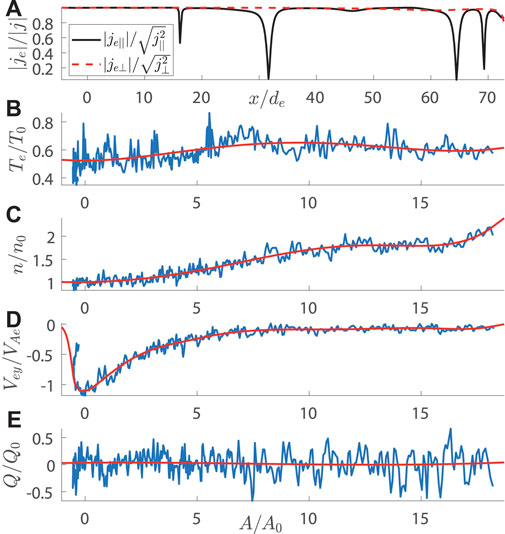
FIGURE 1. Reconstruction of the event of July 11, 2017. The model functions evaluated at the reconstruction region boundary (MMS3 trajectory). Panel (A) represents the ratio of the electron and full currents for parallel (black) and perpendicular (red) in-plane current components vs. the spacecraft travel distance x. Panels (B–E) represent electron temperature, number density, out-of-plane velocity, and the function Q, respectively, vs. magnetic potential, as they were measured (blue) and interpolated (red). The values of the normalization constants, except for Q0, are provided in Section 3.1 of Korovinskiy et al. (2021), while the corresponding value of Q0 = 18.5 s−1cm−3.
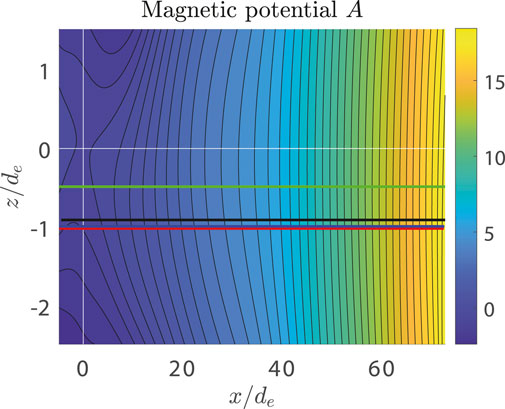
FIGURE 2. Reconstruction of the event of July 11, 2017. The calculations were initiated at the MMS3 trajectory in SCS. The magnetic potential A(x, z) is shown by color, and contour lines plot the in-plane magnetic field lines. The spacecraft trajectories are plotted by black color for MMS1, red for MMS2, green for MMS3, and blue for MMS4. White lines plot the SCS coordinate system. Spacecraft move from the left to the right.
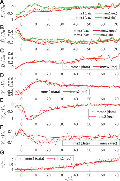
FIGURE 3. Reconstruction of the event of July 11, 2017. The calculations were initiated at the MMS3 trajectory in SCS. The measured values (red and dotted) and the reconstruction results (red and solid) vs. x for Bx (A),
2.3 The fundamental limitations of the EMHD GS reconstruction technique
2.3.1 Two-dimensionality
All the discussed EMHD GS reconstruction techniques possess the obvious fundamental limitations—they assume the 2D steady-state configuration, which can be hardly found in nature. In particular, the abovementioned failure of reconstruction of the normal component of the electron velocity (Vez in our notations) within the internal EDR was claimed a signature of the CS two-dimensionality violation at the ground of simple qualitative speculations (Korovinskiy et al., 2021). Indeed, according to Ampère’s law (2), nVez = ∂Bx/∂y − ∂By/∂x. In the 2D model, the term ∂Bx/∂y is omitted, which can result in considerable error if, in reality, this term is non-zero, because we omit the derivative of Bx – the major magnetic field component (in the LMN coordinate system). This 3D effect should be much less pronounced for the component Vex = (1/n) (∂By/∂z − ∂Bz/∂y) because, here, we neglect the derivative of Bz – the minor magnetic field component. Obviously, the direct evaluation of the derivative ∂Bx/∂y would be the best way to make sure that the failure of Vez reconstruction is caused by the CS three-dimensionality. Such evaluation is hardly possible; however, the following scaling analysis supports the aforementioned speculations. Fortunately, during this particular event, two coordinate systems, SCS and LMN, were very close, differing from each other for 5.8° only (Korovinskiy et al., 2021). This allows adopting the LMN scaling ratios in SCS.
The spacecraft trajectories represent parallel linear segments in the 3D space. In SCS, each of them represents the inclined line (dy/dx ≈ 0.75) belonging to the plane zj = const, where subscript j stands for the probe number. Let us assume that CS is two dimensional, ∂/∂y = 0. Then, the equality ∂Bx/∂x + ∂Bz/∂z = 0 is to fulfil, where ∂Bx/∂x = dBx/dx at any probe trajectory. Since in LMN, ∂/∂z ∼ 1 and ∂/∂x ∼ϵ, we obtain ∂Bx/∂x = −∂2A/∂x∂z ∼ϵ (in the first part of the reconstruction region, within the internal EDR, the magnetic potential A ∼ 1, as seen in Figure 2). With the reconnection rate ER ≈ 0.15–0.2 (Nakamura et al., 2018; Hasegawa et al., 2019; Korovinskiy et al., 2021), one can estimate the numerical value of ϵ ≈ 0.2. Analogously, for the increment of Bz, we have
Now, let us estimate the terms ΔBx/Δx and ΔBz/Δz, where Δ stands for the finite difference. At any probe trajectory, in particular, at the trajectory of MMS2, we have ΔBx/Δx = dBx/dx ∼ϵ, where dx is the grid step. To evaluate the term ΔBz/Δz, we use the data of the two nearest probes, MMS2 and MMS4 (Figure 2), whose trajectories were shifted with respect to each other for Δx = 0.15, Δy = 0.683, and Δz = 0.027. Substituting these values in the formula for dBz, we obtain ΔBz/Δz = ∂Bz/∂z + ∂Bz/∂x ⋅Δx/Δz ∼ϵ + ϵ2/ϵ ∼ϵ, where we used the estimate Δx/Δz ≈ 5.6 ∼ 1/ϵ. So, in the 2D configuration, the terms ΔBx/Δx and ΔBz/Δz, evaluated this way, are to be the quantities of the same order ϵ, matching the order of the corresponding partial derivatives ∂Bx/∂x and ∂Bz/∂z, respectively.
The plot of ΔBz/Δz, exhibited in Figure 4, mismatches this conclusion. In Figure 4, we observe the minor term ΔBy/Δy (evaluated analogously to ΔBz/Δz) with the peaking value of about 0.07, that is, ∼ϵ2 (red), the term ΔBx/Δx with the peaking value
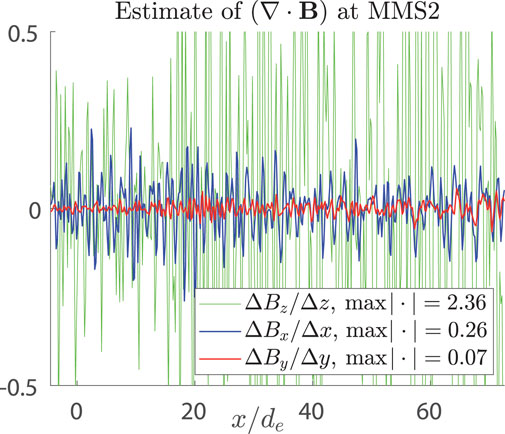
FIGURE 4. Reconstruction of the event of July 11, 2017. The estimate of the terms of (∇ ⋅ B) at the MMS2 trajectory via finite differences ΔBz/Δz (green), ΔBx/Δx (blue), and ΔBy/Δy (red) is plotted vs. the MMS2 path length. The magnitudes are given in the legend.
Thus, we arrive at the following scaling estimates: ∂Bx/∂y ∼ϵ and ∂By/∂x ∼ϵ2. Clearly, neglect of the first (major) term and keeping the second (minor) one result in the Vez reconstruction failure in the left part of the reconstruction interval (Figure 3F). In the right part, by contrast with
It should be noted that since the scaling analysis operates not with the exact but with the typical values, one can be easily misled. For example, with ϵ = 0.2 and
2.3.2 Steady state
The reconstruction of Korovinskiy et al. (2021) has also revealed the signatures of CS time dependence, observed during the first 0.4 s, when the out-of-plane component Ey demonstrated some reduction and the function Vey(A) was not single-valued (see Figures 2A, 3E of the cited paper), which resulted in a low reconstruction accuracy within this interval (see Figure 6 of Korovinskiy et al. (2021) or Figure 3). To investigate the model failure in an unsteady CS, we addressed the event of September 8, 2018, when at nearly 14:51:30 UT, MMS encountered an EDR near the center of a flux-rope type dipolarization front (Marshall et al., 2020). The reconstruction is performed in the co-moving LMN reference frame. The direction of the M-axis is determined by the maximization of the peaking out-of-plane current density, max (jeM), and the N-axis is found by the maximization of the BL variation, where the L-axis completes the right-handed LMN coordinate system. The LMN unit vectors, specified in the Geocentric Solar Ecliptic (GSE) coordinate system, have the following components: eL = [−0.11648, +0.27887, +0.95324], eM = [+0.07826, +0.95936, −0.27110], and eN = [−0.99010, +0.04302, −0.13357]. This LMN coordinate system is nearly the same as the one that was determined by Marshall et al. (2020), differing from the latter mainly by the opposite signs of the M and N orts. The normal component of the structure velocity was determined by the timing method (Russell et al., 1983), and two other components were estimated as the average ion velocity within the 1.5 s reconstruction interval 14.51.30.25–14.51.31.75 UT. This way the value of V0 = [+117.43, +233.92, −251.34] km/s in LMN (which is [+253.48, +246.35, +082.09] km/s in GSE) was derived. All quantities were cast by Lorentz transform to the LMN coordinate system moving with the velocity V0 (co-moving reference frame) and normalized for the typical values of t0 = 0.568 ms, n0 = 1 cm−3, T0 = 497 keV, p0 = 79.6 pPa, de = 5.31 km, B0 = 10 nT, VAe = 9.35 ⋅ 103 km/s, EAe = 93.5 mV/m, and j0 = 1.5 μA/m2. Since in all previous studies, the simplified model (Eq. 8) performed good enough, while the contribution of the terms accounting the dependence of Vey on By was found rather small (Korovinskiy et al., 2020; 2021), we restricted our study to solving Eq. 8.
The reconstruction setup is exhibited in Figure 5, where MMS1-related curves are plotted by black, MMS2 by red, and MMS3 by green in all panels. Panels (A) and (B), respectively, show the out-of-plane electric field and number density vs. time. These plots reveal that (a) number density was not uniform and (b) the steady-state condition Ey = const was fulfilled up to some moment, then it failed abruptly (Ey peaks at t = 1.17 s at the MMS1 trajectory and at t = 1.08 s at the MMS3 one). Magnetic potential A vs. time and the out-of-plane electron current jeM vs. A are plotted in panels (C) and (D), respectively. Similar to the event of July 11, 2017, the non-monotonic behavior of A(t) makes our modelling function jeM(A) double-valued. However, in the study of Korovinskiy et al. (2021), a single-valued analytical continuation of the necessary function could be constructed, since the general appearance of the required curve was evident. In the present case, it is not so. Basically, with the function jeM(A), shown in Figure 5D, the reconstruction is not possible.
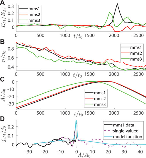
FIGURE 5. Reconstruction of the event of September 8, 2018. The calculations are performed in the co-moving LMN coordinate system. In all panels, the data are plotted by black color for MMS1, by red for MMS2, and by green for MMS3. Panels (A,B), respectively, show the out-of-plane electric field EM and the number density n vs. time. Magnetic potential A vs. time and the out-of-plane electron current density jeM vs. A are plotted in panels (C,D), respectively. A single-valued function j′(A) at the MMS1 trajectory, obtained by flipping one of the branches of the double-valued jeM(A) with respect to the branching point, is plotted in panel (D) by dashed magenta curve, and the interpolating function, used in reconstruction, is shown by the solid cyan curve. The data of MMS4 are not shown for better visibility, the same for data of MMS2 and MMS3 in panel (D).
Nevertheless, BLA allows one trick, resting upon two features and one assumption, which are: (a) magnetic potential is defined with the accuracy of an arbitrary constant; (b) in BLA, the derivatives on x are neglected, hence in any particular vertical cross section, we solve the one-dimensional problem; and (c) since the out-of-plane current is a sharply peaking function, we assume that in some vicinity of the peak, it can be approximated by a symmetrical (Gauss-like) curve. By making use of properties (a) and (b), and adopting assumption (c), we can “unfold” two coalescent branches of jeM(A). Namely, we make the substitution A − a0 → A, where a0 is the point of branching. Then, one branch (in our case, the first one, corresponding to the initial steady period) is flipped with respect to the axis A = 0. This means that for any vertical cross section rL = rLj, where j is the point number, we make the substitution Aj → −Aj (rL and rN correspond, respectively, to x and z of the analytical model). This way we obtain a single-valued function j′(A), whose interpolated value is used for solving Eq. 8; then, in each vertical cross section, the reverse substitution A− 2Aj → A is performed. For MMS1-based reconstruction, the function j′(A) and its interpolated values are shown in Figure 5D by dashed magenta and solid cyan curves, respectively. The validity of such approach is obviously predicated upon the validity of assumption (c) and by the accuracy of the LMN coordinate system detection.
The results of reconstruction in the 0.32 s timespan (t = 0.92:1.24 s) are plotted in Figure 6. For reconstruction, initiated at the MMS1 trajectory, a 2D contour plot of magnetic potential and the L-component of the magnetic field is plotted in panels (A) and (B), respectively. For reconstruction, initiated at the MMS3 trajectory, the same quantities are plotted in panels (C) and (D). Since MMS spacecraft (moving from the right to the left) are not aligned in a single vertical line, the plots of panels (A) and (C) demonstrate the time evolution of the CS. Indeed, the colored asterisks in panel (A) mark the spacecraft mutual locations at a single moment. Starting reconstruction, e.g., from the black asterisk, we cross the MMS3 trajectory (green line) at the moment, when MMS3 has already passed farther, and the other way round. Particularly, in panel (C), MMS3 crosses the O-line with two X-lines, one on the right and one on the left. In panel (A), we see the same structure, though shifted to the left and deformed. The magnetic components BL, shown in panels (B) and (D), demonstrate that the trusted reconstruction area, if it is, spans between the MMS1 and MMS3 trajectories, while at the trajectories of MMS2 and MMS4, the reconstruction error becomes too big, which is reasonable since the latter probes are more remote. Comparing the solid and dashed green curves in Figure 6B, we see that the reconstruction of the magnetic field component BL at MMS3 exhibits appropriate accuracy in the right part of the reconstruction region, rL > − 20 (initial period). It means that real existence of the X-line, as shown in Figure 6A at (rL, rN) ≈ (−20, 40) may be questionable. The existence of the X-line, crossed by MMS1 in Figure 6C at rL ≈ − 23, may be claimed more certainly, since the black solid and dashed curves in Figure 6D assure good reconstruction accuracy at MMS1 for rL < − 22. One can also see that our LMN coordinate system does match the magnetic configuration geometry in the vicinity of the X-point, encountered by MMS1. The existence of the X-line between MMS3 and MMS4 at xL ≈ − 17, also observed in Figure 6C, requires additional verification by means of some other method, since the comparison of blue solid and dashed curves in Figure 6D does not lead to any unequivocal conclusion.
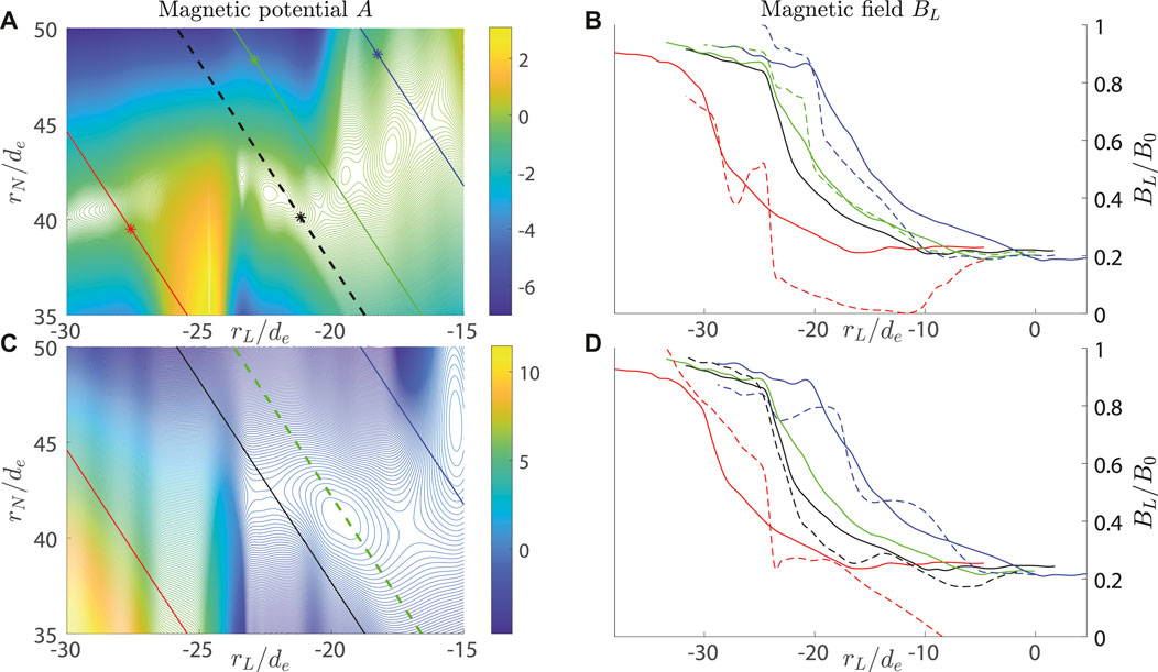
FIGURE 6. Reconstruction of the event of September 8, 2018, in the co-moving LMN coordinate system. Top row: the results of reconstruction initiated at the MMS1 trajectory. The 2D contour plot of the magnetic potential and the L-component of the magnetic field are plotted in panels (A,B), respectively. In the bottom row, the same quantities are plotted in panels (C,D) for the reconstruction initiated at the MMS3 trajectory. The spacecraft trajectories in the left column are plotted by black color for MMS1, red for MMS2, green for MMS3, and blue for MMS4, where dashed lines plot the reconstruction domain boundary. In the right column, the spacecraft data (solid) and the reconstructed values (dashed) at four MMS probes are plotted by the same colors. In panel (A), the colored asterisks demonstrate the spacecraft mutual locations at a single moment (probes move from the right to the left).
The results of Section 2.3 reveal that the 2D steady-state model demonstrates remarkable ability to withstand (to some extent) the violation of the ideal CS conditions, i.e., the violation of both fundamental model limitations. With some gimmickries, the model is capable of providing an overview of the reconnection region even for the time-dependent reconnection event. However, for such events, of course, it would be much better to use some time-depended model, such as those of Denton et al. (2020, 2021).
2.4 Perspectives of the EMHD GS reconstruction technique improvement
Apart from the fundamental limitations discussed previously, the existing EMHD GS techniques also possess some minor limitations which can be coped with (to some extent) in the future studies. Particularly, such limitations are stipulated by the simplifying assumptions adopted for the model functions. Such simplifications ease the calculations but shrink the models’ applicability domain. For example, the assumption of n = const is appropriate within the internal EDR only. The less strict condition n = n(A) allows the considerable expansion of the reconstruction region in the longitudinal direction onto the external EDR; however, the cross size of this region stays rather small, as shown in Figure 10A of Korovinskiy et al. (2020). Also, as for the approximation Vey = Vey(A), it seems to be violated nearly everywhere within the internal EDR (see Figure 10B of the cited paper). The correct model would consider all magnetoplasma quantities as functions of two variables (A, By). This cannot be applied directly due to the lack of the input data, but this correct treatment may be approached by using a polynomial technique, bearing some similarity to those of Denton et al. (2022), but operating in another variable space. In this section, we present an analytical frame for such extension of A2 [Model 2 of Korovinskiy et al. (2021)] and the recipe to unite A1 and A2 to benefit from the advantages of these two approaches and to master their disadvantages.
To proceed to this goal, one needs to cast the problem (1–5, 9) in another form. Partly, this work was made in the studies of Korovinskiy et al. (2020, 2021), which results we outline here, omitting all intermediate details. The Jakobian of the variables transform (x, z) → (A, By) is
where we introduce the notation ɛ* for the out-of-plane component of the electron convective electric field,
while ɛ is the normalized value of the out-of-plane electric field Ey. The most general form of Eq. 10 takes the form
We also introduce the notation φ* for the quantity, which we call the “effective electric potential”,
where φ(A, By) is the electric potential of the in-plane electric field: Ex = −∂φ/∂x, Ez = −∂φ/∂z. The problem for φ* is stated in two equations:
where the electron inertia and anisotropy are accounted by the term R [see Eqs 14, 15 of Korovinskiy et al. (2021)],
Multiplying (21) for ∇A and (22) for ∇By, we obtain the equation for ∇φ*:
Differentiating (21) for By and (22) for A and equating the results, we obtain the equation for Vey. By using (23), it takes the following form:
Let us consider Eqs 21, 22, where the terms n, Te, and Vey are of the order of 1 due to normalization (Figure 1), the term
2.4.1 Reconstruction in a thin layer
Equation 25 provides us with the condition of the model self-consistency and gives a clue to the first step for model generalization. The rightmost term of this equation vanishes under the following assumptions:
while Eq. 25 itself takes the following form:
Assumptions (26) are expected to be relevant in a thin current layer spanning both the internal and external EDR, though the cross size of the model applicability domain will highly likely not exceed several de [see Figure 10 in Korovinskiy et al. (2020) and the corresponding discussion]. Adopting assumptions (26) and utilizing BLA, i.e., neglecting the second-order terms, Eqs 8, 19, 24 make the following system:
According to (7), the last term of the definition
where the sum in the right-hand side of (32) represents the Taylor series for the vorticity component
and by equating the terms containing the same powers of
where k = {3, 4, … }. Assuming that coefficients ωl(A) for l = {0, 1, … , N − 1} are found, the coefficients {V1, … , VN} are evaluated, and V0(A) is calculated from the boundary conditions as a difference between the data and the truncated Taylor series,
where ωlm are the numerical constants. Thus, the representation for the vorticity takes the following form:
Analogous to V0(A), the term ω0(A) is evaluated from the boundary conditions, ω0(A) = ωey − δω, when coefficients ωlm are known. The coefficients ωlm are found by solving the boundary value problem (BVP) for the system (28–30). The number of coefficients, which can be found this way, is equal to the number of extra conditions imposed. At the capacity of these conditions, one can use some limiting values of the peaking or average reconstruction error for the calculated quantities. The solution of the system (28–30) provides us with the values of 10 quantities: n, Te, B, Ve, Ex, and Ez. However, the quantities Ex, Bz, and Vez cannot provide us with the fiducial markers, since not an exact but the regularized problem is solved, so that only seven quantities are left in the control list. Since both n and Te are assumed to depend only on A, it is reasonable to eliminate one of these quantities from the list also. Assuming that the data of all four MMS spacecraft are available, we have 24 extra conditions, which are enough for developing the sixth-order reconstruction scheme
It should be noted that the term ω0(A) can also be represented in a form of the truncated Taylor series. In this case, the coefficients of this series enlarge the number of unknowns. This reduces the maximal order of the scheme to five, but allows the problem solution when the data on the velocity derivatives are unreliable (too noisy) or unavailable. In this case, it may be convenient to modify the technique by reversing relations (34).
Then, Vey is presented in the form analogous to (35–37), and numerical coefficients Vkm and the integration constants of Eq. 38 are found from the solution of the same BVP.
2.4.2 The general case
In the most general case, all quantities are to be considered as functions of two variables,
Since n depends on
where the subscript bc stands for the boundary conditions and
2.4.3 The SCS-tailored technique
As needed, the described technique may be easily tailored for calculations in the SCS x′yz′, presenting the rotated co-moving LMN coordinate system, where the x′-axis coincides with the satellite trajectory and the z′-axis is normal to it. To this end, the neglected terms of the considered equations are to be kept. Particularly, Eqs 39, 40 take the following form:
where we omitted superscript ′ at all entries of x and z for shortening the notations, while the y-components and potentials are invariant with respect to the coordinate system rotating around the y axis. Eq. 41 does not change, but the term
Equations 45, 46 do not contain any term requiring the calculation of some extra coefficients as compared to Eqs 39, 40; hence, the same Taylor series technique is applied for solving these equations. However, in SCS, the quantities Bz, Ex, and Vez augment the control list; hence, we have 12 extra control conditions (if all four MMS probes are in play). With representation (42–44) and 12 additional coefficients, one can build the fourth-order scheme (40 coefficients in total) for the system (41, 45, 46). In contrast with the third-order scheme, in the fourth-order scheme, the quantity Q0(A) cannot be represented in a form of the Taylor series, since such representation would require five coefficients more, while we can calculate only four by using Eq. 25, which specifies one extra control condition at each spacecraft trajectory. An additional condition q00 = 0, expressing the reasonable assumption of the absence of the constant term, makes such representation available.
3 Results
In the present study, we investigate the technique of EMHD GS reconstruction of the 2D steady-state reconnection kernel region, namely, the EDR. We discuss two families of models, which we call A1 (Sonnerup et al., 2016; Hasegawa et al., 2017; 2019; 2021) and A2 (Korovinskiy et al., 2020; 2021) in terms of comparison of their advantages and disadvantages. A1 represents a more universal technique, appropriate for arbitrary orientation of the spacecraft trajectory with respect to the EDR. It requires single probe data to setup the calculations. A2 is simpler but less universal, it is not appropriate for vertical crossings and it requires at least two probes to evaluate the boundary conditions. Both models, as they are developed for today, adopt some (different) simplifying assumptions, restricting the applicability domain. One of these assumptions, the constancy of number density, adopted in Model 2 of Korovinskiy et al. (2021), is released, and this new compressible model is tested by reconstructing the event of Torbert et al. (2018). This allowed three times expansion of the reconstruction interval as compared to previous studies (Hasegawa et al., 2019; Korovinskiy et al., 2021).
The fundamental limitations of the 2D steady-state treatment are considered in terms of the reconstruction inaccuracy that emerges when this simplified approach is utilized for the reconstruction of real EDRs in Earth’s magnetotail. Particularly, the reconstruction of the event of July 11, 2017, demonstrated the remarkable robustness of the reconstruction technique A2 with respect to the violation of the configuration two-dimensionality. It is found that weak 3D effects (∂/∂y ∼ϵ) do not ruin the reconstruction scheme, crashing the reconstruction of the minor (normal to CS) electron velocity component only, but not the other quantities. The productivity of the EMHD GS technique in the unsteady reconnection region reconstruction is tested by means of Marshall et al.’s (2020) event. The reconstruction results agreed with the conclusion of Marshall et al. (2020) concerning the duration of the reconnection region crossing of about 0.3 s. The X-line between MMS1 and MMS2, reported by Marshall et al. (2020), is also observed in our reconstruction and is found to be close to the MMS1 trajectory. Additionally, the O-line at the MMS3 trajectory and the X-line between MMS3 and MMS4 (Figure 6C), moving toward MMS1 (Figure 6A), are also discovered. However, the abrupt break of the steady state makes the reconstruction-trusted interval too small (of the order of the distance between MMS1 and MMS3 trajectories, i.e.,
The perspectives of improving the existing EMHD GS reconstruction models are studied analytically. The presented study has shown that the self-consistent EDR reconstruction model for the EMHD system (1–5, 9), adoptable for arbitrary-oriented multi-probe mission (MMS or future multi-spacecraft missions capable of resolving the electron-scale physics) crossings, can be developed without using any singular equation and/or simplified model for the electron pressure anisotropy term
4 Discussion
In a general sense, EMHD GS reconstruction of any reconnection event represents a complex problem, where reconstruction itself is a final step, which is preceded by the in situ data analysis and event identification, estimate the structure velocity (V0) and the proper LMN coordinate system. Discussing all these aspects goes beyond the scope of the present study, where we focus on the reconstruction problem in a strict sense. Since two magnetotail reconnection events, addressed in this study, have been introduced previously, for the omitted details, we refer the reader to the corresponding studies of Hasegawa et al. (2019); Marshall et al. (2020); and references therein. In particular, the reconstruction setup in Section 2.2.3 is fully identical to those of Hasegawa et al. (2019); Korovinskiy et al. (2021), which is made to facilitate the results comparison. The setup of Section 2.3.2 differs from the data of Marshall et al. (2020) mainly by the value of V0, since in the cited study, the latter was estimated too rough. In terms of the event study, the accurate estimate of V0 is important since it specifies the relative motion of the spacecraft to the structure (spacecraft trajectory). However, in terms of the study of the reconstruction model efficiency, the accuracy of the V0 estimate is less important since this estimate affects the spacecraft trajectory, hence the model functions and the geometry of the reconstructed magnetic configuration, but neither its topology nor the accuracy of the magnetoplasma quantities reconstruction.
The EMHD GS reconstruction has got its name due to Eq. 8, representing a zero-order scheme for evaluating the magnetic potential A. Meanwhile, the accurate consideration of the problem demands solving the two-dimensional problem, since in steady-state 2D configuration all magnetoplasma quantities stay functions of two variables, whatever variable space is considered. However, in some coordinate systems, these two independent variables are not peer in terms of scaling. Particularly, in the co-moving LMN coordinate system, where the z-axis coincides with the CS normal direction, the scaling ratios ∂/∂z ∼ 1 and ∂/∂x ∼ϵ≪ 1 allow considerable simplification of equations by neglecting the minor terms ∼ϵ2 with respect to the major ones
Development of such schemes by means of the polynomial technique is considered in Section 2.4. The suggested method benefits from the usage of both BLA and rotationally invariant coordinates
The further advantage of EMHD GS reconstruction stems from the fact that the equation of the ion motion splits from the system (1–5, 9). It means that ions move in the applied field, and the ion bulk velocity is evaluated when other magnetoplasma quantities are found. The simplified problem analysis is given in Korovinskiy et al. (2008). Under proper generalization, the analogous approach can be applied in the extended reconstruction models A1 and A2. This, in turn, provides the opportunity of analytical studies of the ion motion in the SR in view of such high-impacting factors as ion mass, temperature, and distance to X-line, affecting both ion heating and acceleration (Zaitsev et al., 2021). For example, the ion mass appears to be a crucial parameter for the kinetic energy gain because of the assumed energization condition |mi∇E⊥/(eB2)| > 1 (Cole, 1976). The temperature of the cold ion fraction is also of high importance because these ions may change the reconnection rate (André and Cully, 2012), reduce the Hall current (André et al., 2016; Dargent et al., 2017), and change the energy budget of magnetic reconnection (Toledo-Redondo et al., 2017). At last, the distance to X-line is of high importance because the reconnection electric field, driving cold ions inside the exhaust without thermalization, exists only between the X-line and the pileup front (Alm et al., 2018; Toledo-Redondo et al., 2018), on the contrary to the Hall electric fields that presents in the entire SR.
The less evident, EMHD GS reconstruction can be utilized for studies of the kinetic (Pritchett and Coroniti, 2010) or MHD (Sorathia et al., 2020) ballooning-interchange (BI) instability, explaining the appearance of auroral beads and related ionospheric current disturbances in the late substorm growth phase (Panov et al., 2019; Sorathia et al., 2020). More specifically, this method may be applied for studies of BI heads, which are located in the near-Earth plasma sheet at the distances of 7–14 Earth’s radii downtail, where they can drift in both dusk and dawn directions (Panov et al., 2012; Panov and Pritchett, 2018a). Indeed, the kinetic BI mode is identified as the low-frequency extension in a curved magnetic geometry of the lower-hybrid-drift instability in straight magnetic fields (Pritchett and Coroniti, 2010; 2011; 2013) with |ji/je|∼ 0.2 (Panov and Pritchett, 2018a; b). Thus, BI heads represent slowly varying (as compared to the electron plasma frequency) quasi-2D structures (oriented in the equatorial plane) governed by the electron currents, i.e., they fulfil all the basic assumptions of the EMHD GS reconstruction models. The reconstruction of the proper in situ data would provide an insight to morphology of the BI heads and ion motion driving mechanisms. In particular, the problem of the primary driver of the ion motion in BI heads (the Hall electric field or the ion proper buoyancy) could be addressed.
Apart from providing an intermediate step between satellite data and numerical simulations, EMHD GS reconstruction also allows the analysis of various electron-scale structures in terms of their key parameters, such as plasma β, entropy, magnetic field curvature, and electron kinetic scales. The present study demonstrates the significant potential of this method both in terms of the increase of physical accuracy and in terms of model scope expansion. The furthest improvement of the EMHD GS technique assumes the generalization of the reconstruction model for fully anisotropic electron pressure and temperature, which stays a challenging problem for future studies.
Data availability statement
Publicly available datasets were analyzed in this study. The MMS data used here are available from the MMS Science Data Center: https://lasp.colorado.edu/mms/sdc/public/.
Author contributions
All authors listed have made a substantial, direct, and intellectual contribution to the work and approved it for publication.
Funding
This study has been supported by the Austrian Science Fund (FWF): I 3506-N27 and Austrian FFG project ASAP15/873685.
Acknowledgments
The authors thank the Editor and the Reviewers for their help in improving the manuscript.
Conflict of interest
The authors declare that the research was conducted in the absence of any commercial or financial relationships that could be construed as a potential conflict of interest.
Publisher’s note
All claims expressed in this article are solely those of the authors and do not necessarily represent those of their affiliated organizations, or those of the publisher, the editors, and the reviewers. Any product that may be evaluated in this article, or claim that may be made by its manufacturer, is not guaranteed or endorsed by the publisher.
References
Alm, L., Andre, M., Vaivads, A., Khotyaintsev, Y. V., Torbert, R. B., Burch, J. L., et al. (2018). Magnetotail hall physics in the presence of cold ions. Geophys. Res. Lett. 45, 10–941. doi:10.1029/2018GL079857
André, M., and Cully, C. M. (2012). Low-energy ions: A previously hidden solar system particle population. Geophys. Res. Lett. 39. doi:10.1029/2011GL050242
André, M., Li, W., Toledo-Redondo, S., Khotyaintsev, Y. V., Vaivads, A., Graham, D. B., et al. (2016). Magnetic reconnection and modification of the Hall physics due to cold ions at the magnetopause. Geophys. Res. Lett. 43, 6705–6712. doi:10.1002/2016GL069665
Aunai, N., Belmont, G., and Smets, R. (2011). Energy budgets in collisionless magnetic reconnection: Ion heating and bulk acceleration. Phys. Plasmas 18, 122901. doi:10.1063/1.3664320
Bagenal, F. (2013). Planetary magnetospheres. Dordrecht, Netherlands: Springer, 251–307. doi:10.1007/978-94-007-5606-9_6
Bessho, N., Chen, L.-J., Wang, S., Hesse, M., and Wilson, L. (2019). Magnetic reconnection in a quasi-parallel shock: Two-dimensional local particle-in-cell simulation. Geophys. Res. Lett. 46, 9352–9361. doi:10.1029/2019GL083397
Bhattacharjee, A. (2004). Impulsive magnetic reconnection in the Earth’s magnetotail and the Solar corona. Annu. Rev. Astron. Astrophys. 42, 365–384. doi:10.1146/annurev.astro.42.053102.134039
Birn, J., Drake, J., Shay, M., Rogers, B., Denton, R., Hesse, M., et al. (2001). Geospace Environmental Modeling (GEM) magnetic reconnection challenge. J. Geophys. Res. Space Phys. 106, 3715–3719. doi:10.1029/1999JA900449
Birn, J., and Hesse, M. (2010). Energy release and transfer in guide field reconnection. Phys. Plasmas 17, 012109. doi:10.1063/1.3299388
Bulanov, S., Pegoraro, F., and Sakharov, A. (1992). Magnetic reconnection in electron magnetohydrodynamics. Phys. Plasmas 4, 2499–2508. doi:10.1063/1.860467
Burch, J., Hesse, M., Webster, J., Genestreti, K., Torbert, R., Denton, R., et al. (2022). The EDR inflow region of a reconnecting current sheet in the geomagnetic tail. Phys. Plasmas 29, 052903. doi:10.1063/5.0083169
Burch, J., Moore, T., Torbert, R., and Giles, B. (2016). Magnetospheric multiscale overview and science objectives. Space Sci. Rev. 199, 5–21. doi:10.1007/s11214-015-0164-9
Cai, H.-J., and Lee, L. (1997). The generalized Ohm’s law in collisionless magnetic reconnection. Phys. Plasmas 4, 509–520. doi:10.1063/1.872178
Cassak, P., Baylor, R., Fermo, R., Beidler, M., Shay, M., Swisdak, M., et al. (2015). Fast magnetic reconnection due to anisotropic electron pressure. Phys. Plasmas 22, 020705. doi:10.1063/1.4908545
Cassak, P., and Fuselier, S. (2016)., 427. Springer, 213–276. of Astrophys. doi:10.1007/978-3-319-26432-5_6Reconnection at Earth’s dayside magnetopauseSpace Sci. Lib.
Cassak, P., Liu, Y.-H., and Shay, M. (2017). A review of the 0.1 reconnection rate problem. J. Plasm. Phys. 83, 715830501. doi:10.1017/S0022377817000666
Chen, L.-J., Wang, S., Le Contel, O., Rager, A., Hesse, M., Drake, J., et al. (2020). Lower-hybrid drift waves driving electron nongyrotropic heating and vortical flows in a magnetic reconnection layer. Phys. Rev. Lett. 125, 025103. doi:10.1103/PhysRevLett.125.025103
Chen, Y., and Hu, Q. (2022). Small-scale magnetic flux ropes and their properties based on in situ measurements from the parker solar probe. Astrophys. J. 924, 43. doi:10.3847/1538-4357/ac3487
Cole, K. (1976). Effects of crossed magnetic and (spatially dependent) electric fields on charged particle motion. Planet. Space Sci. 24, 515–518. doi:10.1016/0032-0633(76)90096-9
Comisso, L., and Bhattacharjee, A. (2016). On the value of the reconnection rate. J. Plasm. Phys. 82, 595820601. doi:10.1017/S002237781600101X
Cozzani, G., Khotyaintsev, Y. V., Graham, D. B., Egedal, J., André, M., Vaivads, A., et al. (2021). Structure of a perturbed magnetic reconnection electron diffusion region in the Earth’s magnetotail. Phys. Rev. Lett. 127, 215101. doi:10.1103/PhysRevLett.127.215101
Dargent, J., Aunai, N., Lavraud, B., Toledo-Redondo, S., Shay, M., Cassak, P., et al. (2017). Kinetic simulation of asymmetric magnetic reconnection with cold ions. J. Geophys. Res. Space Phys. 122, 5290–5306. doi:10.1002/2016JA023831
Daughton, W., Nakamura, T., Karimabadi, H., Roytershteyn, V., and Loring, B. (2014). Computing the reconnection rate in turbulent kinetic layers by using electron mixing to identify topology. Phys. Plasmas 21, 052307. doi:10.1063/1.4875730
Daughton, W., Scudder, J., and Karimabadi, H. (2006). Fully kinetic simulations of undriven magnetic reconnection with open boundary conditions. Phys. Plasmas 13, 072101. doi:10.1063/1.2218817
Denton, R. E., Liu, Y.-H., Hasegawa, H., Torbert, R. B., Li, W., Fuselier, S., et al. (2022). Polynomial reconstruction of the magnetic field observed by multiple spacecraft with integrated velocity determination. J. Geophys. Res. Space Phys. 127, e2022JA030512. doi:10.1029/2022JA030512
Denton, R. E., Torbert, R. B., Hasegawa, H., Genestreti, K. J., Manuzzo, R., Belmont, G., et al. (2021). Two-dimensional velocity of the magnetic structure observed on july 11, 2017 by the magnetospheric multiscale spacecraft. J. Geophys. Res. Space Phys. 126, e2020JA028705. doi:10.1029/2020JA028705
Denton, R., Sonnerup, B. Ö., Russell, C., Hasegawa, H., Phan, T.-D., Strangeway, R., et al. (2018). Determining <i>L</i> - <i>M</i> - <i>N</i> current sheet coordinates at the magnetopause from magnetospheric multiscale data. J. Geophys. Res. Space Phys. 123, 2274–2295. doi:10.1002/2017JA024619
Denton, R., Torbert, R., Hasegawa, H., Dors, I., Genestreti, K., Argall, M., et al. (2020). Polynomial reconstruction of the reconnection magnetic field observed by multiple spacecraft. J. Geophys. Res. Space Phys. 125, e2019JA027481. doi:10.1029/2019JA027481
Divin, A., Markidis, S., Lapenta, G., Semenov, V., Erkaev, N., and Biernat, H. (2010). Model of electron pressure anisotropy in the electron diffusion region of collisionless magnetic reconnection. Phys. Plasmas 17, 122102. doi:10.1063/1.3521576
Divin, A., Semenov, V., Korovinskiy, D., Markidis, S., Deca, J., Olshevsky, V., et al. (2016). A new model for the electron pressure nongyrotropy in the outer electron diffusion region. Geophys. Res. Lett. 43, 10,565–10,573. doi:10.1002/2016GL070763
Divin, A., Semenov, V., Zaitsev, I., Korovinskiy, D., Deca, J., Lapenta, G., et al. (2019). Inner and outer electron diffusion region of antiparallel collisionless reconnection: Density dependence. Phys. Plasmas 26, 102305. doi:10.1063/1.5109368
Dorfman, S., Ji, H., Yamada, M., Yoo, J., Lawrence, E., Myers, C., et al. (2013). Three-dimensional, impulsive magnetic reconnection in a laboratory plasma. Geophys. Res. Lett. 40, 233–238. doi:10.1029/2012GL054574
Drake, J., Swisdak, M., Phan, T., Cassak, P., Shay, M., Lepri, S., et al. (2009). Ion heating resulting from pickup in magnetic reconnection exhausts. J. Geophys. Res. Space Phys. 114, A05111. doi:10.1029/2008JA013701
Du, S., Guo, F., Zank, G. P., Li, X., and Stanier, A. (2018). Plasma energization in colliding magnetic flux ropes. Astrophys. J. 867, 16. doi:10.3847/1538-4357/aae30e
Dungey, J. (1953). LXXVI. Conditions for the occurrence of electrical discharges in astrophysical systems. Lond. Edinb. Dublin Philosophical Mag. J. Sci. 44, 725–738. doi:10.1080/14786440708521050
Eastwood, J., Phan, T., Øieroset, M., and Shay, M. (2010). Average properties of the magnetic reconnection ion diffusion region in the Earth’s magnetotail: The 2001–2005 Cluster observations and comparison with simulations. J. Geophys. Res. Space Phys. 115. doi:10.1029/2009JA014962
Egedal, J., Le, A., and Daughton, W. (2013). A review of pressure anisotropy caused by electron trapping in collisionless plasma, and its implications for magnetic reconnection. Phys. Plasmas 20, 061201. doi:10.1063/1.4811092
Egedal, J., Le, A., Daughton, W., Wetherton, B., Cassak, P., Chen, L., et al. (2016). Spacecraft observations and analytic theory of crescent-shaped electron distributions in asymmetric magnetic reconnection. Phys. Rev. Lett. 117, 185101. doi:10.1103/PhysRevLett.117.185101
Egedal, J., Ng, J., Le, A., Daughton, W., Wetherton, B., Dorelli, J., et al. (2019). Pressure tensor elements breaking the frozen-in law during reconnection in Earth’s magnetotail. Phys. Rev. Lett. 123, 225101. doi:10.1103/PhysRevLett.123.225101
Egedal, J., Øieroset, M., Fox, W., and Lin, R. (2005). In situ discovery of an electrostatic potential, trapping electrons and mediating fast reconnection in the Earth’s magnetotail. Phys. Rev. Lett. 94, 025006. doi:10.1103/PhysRevLett.94.025006
Fadanelli, S., Lavraud, B., Califano, F., Cozzani, G., Finelli, F., and Sisti, M. (2021). Energy conversions associated with magnetic reconnection. J. Geophys. Res. Space Phys. 126, e2020JA028333. doi:10.1029/2020JA028333
Fu, H., Cao, J., Cao, D., Wang, Z., Vaivads, A., Khotyaintsev, Y. V., et al. (2019a). Evidence of magnetic nulls in electron diffusion region. Geophys. Res. Lett. 46, 48–54. doi:10.1029/2018GL080449
Fu, H., Cao, J., Vaivads, A., Khotyaintsev, Y. V., Andre, M., Dunlop, M., et al. (2016). Identifying magnetic reconnection events using the FOTE method. J. Geophys. Res.: Space Phys. 121, 1263–1272. doi:10.1002/2015JA021701
Fu, H., Vaivads, A., Khotyaintsev, Y. V., Andre, M., Cao, J., Olshevsky, V., et al. (2017). Intermittent energy dissipation by turbulent reconnection. Geophys. Res. Lett. 44, 37–43. doi:10.1002/2016GL071787
Fu, H., Vaivads, A., Khotyaintsev, Y. V., Olshevsky, V., Andre, M., Cao, J., et al. (2015). How to find magnetic nulls and reconstruct field topology with MMS data?. J. Geophys. Res.: Space Phys. 120, 3758–3782. doi:10.1002/2015JA021082
Fu, H., Xu, Y., Vaivads, A., and Khotyaintsev, Y. (2019b). Super-efficient electron acceleration by an isolated magnetic reconnection. Astrophys. J. 870, L22. doi:10.3847/2041-8213/aafa75
Fujimoto, K. (2006). Time evolution of the electron diffusion region and the reconnection rate in fully kinetic and large system. Phys. Plasmas 13, 072904. doi:10.1063/1.2220534
Furth, H. P., Killeen, J., and Rosenbluth, M. N. (1963). Finite-resistivity instabilities of a sheet pinch. Phys. Fluids 6, 459–484. doi:10.1063/1.1706761
Genestreti, K., Burch, J., Cassak, P., Torbert, R., Ergun, R., Varsani, A., et al. (2017). The effect of a guide field on local energy conversion during asymmetric magnetic reconnection: MMS observations. J. Geophys. Res. Space Phys. 122, 11–342. doi:10.1002/2017JA024247
Genestreti, K. J., Varsani, A., Burch, J. L., Cassak, P. A., Torbert, R. B., Nakamura, R., et al. (2018b). MMS observation of asymmetric reconnection supported by 3-D electron pressure divergence. J. Geophys. Res. Space Phys. 123, 1806–1821. doi:10.1002/2017JA025019
Genestreti, K., Nakamura, T., Nakamura, R., Denton, R., Torbert, R., Burch, J., et al. (2018a). How accurately can we measure the reconnection rate em for the mms diffusion region event of 11 July 2017? J. Geophys. Res. Space Phys. 123, 9130–9149. doi:10.1029/2018JA025711
Goldman, M., Newman, D., and Lapenta, G. (2016). What can we learn about magnetotail reconnection from 2D PIC Harris-sheet simulations? Space Sci. Rev. 199, 651–688. doi:10.1007/s11214-015-0154-y
Gonzalez, W., and Parker, E. (2016). Magnetic reconnection, vol. 427 of astrophys. And space sci. Lib. Springer. doi:10.1007/978-3-319-26432-5
Gosling, J., Asbridge, J., Bame, S., Feldman, W., Paschmann, G., Sckopke, N., et al. (1982). Evidence for quasi-stationary reconnection at the dayside magnetopause. J. Geophys. Res. Space Phys. 87, 2147–2158. doi:10.1029/JA087iA04p02147
Grad, H., and Rubin, H. (1958). Hydromagnetic equilibria and force-free fields. J. Nucl. Energy 7, 284–285. doi:10.1016/0891-3919(58)90139-6
Hadamard, J. (1923). Lectures on Cauchy’s problem in linear partial differential equations. New Haven Yale University Press.
Hasegawa, H., Denton, R. E., Nakamura, R., Genestreti, K. J., Nakamura, T. K. M., Hwang, K.-J., et al. (2019). Reconstruction of the electron diffusion region of magnetotail reconnection seen by the MMS spacecraft on 11 July 2017. J. Geophys. Res. Space Phys. 124, 122–138. doi:10.1029/2018JA026051
Hasegawa, H., Nakamura, T. K. M., and Denton, R. E. (2021). Reconstruction of the electron diffusion region with inertia and compressibility effects. J. Geophys. Res. Space Phys. 126, e2021JA029841. doi:10.1029/2021JA029841
Hasegawa, H., Sonnerup, B. U., Denton, R. E., Phan, T.-D., Nakamura, T. K. M., Giles, B. L., et al. (2017). Reconstruction of the electron diffusion region observed by the Magnetospheric Multiscale spacecraft: First results. Geophys. Res. Lett. 44, 4566–4574. doi:10.1002/2017GL073163
Hau, L., and Sonnerup, B. U. Ö. (1999). Two-dimensional coherent structures in the magnetopause: Recovery of static equilibria from single-spacecraft data. J. Geophys. Res. Space Phys. 104, 6899–6917. doi:10.1029/1999ja900002
Hesse, M., and Cassak, P. (2020). Magnetic reconnection in the space sciences: Past, present, and future. J. Geophys. Res. Space Phys. 125, e25935. doi:10.1029/2018JA025935
Hesse, M., Schindler, K., Birn, J., and Kuznetsova, M. (1999). The diffusion region in collisionless magnetic reconnection. Phys. Plasmas 6, 1781–1795. doi:10.1063/1.873436
Hesse, M., and Winske, D. (1998). Electron dissipation in collisionless magnetic reconnection. J. Geophys. Res. 103, 26479–26486. doi:10.1029/98JA01570
Heyn, M. F., and Semenov, V. S. (1996). Rapid reconnection in compressible plasma. Phys. Plasmas 3, 2725–2741. doi:10.1063/1.871723
Hietala, H., Artemyev, A., and Angelopoulos, V. (2017). Ion dynamics in magnetotail reconnection in the presence of density asymmetry. J. Geophys. Res. Space Phys. 122, 2010–2023. doi:10.1002/2016JA023651
Holmes, J., Nakamura, R., Schmid, D., Nakamura, T., Roberts, O., and Vörös, Z. (2021). Wave activity in a dynamically evolving reconnection separatrix. J. Geophys. Res. Space Phys. 126, e2020JA028520. doi:10.1029/2020JA028520
Hoshino, M., Mukai, T., Yamamoto, T., and Kokubun, S. (1998). Ion dynamics in magnetic reconnection: Comparison between numerical simulation and Geotail observations. J. Geophys. Res. Space Phys. 103, 4509–4530. doi:10.1029/97JA01785
Hosner, M., Nakamura, R., Schmid, D., Nakamura, T., Panov, E., and Korovinskiy, D. (2022). Investigation of the evolution of energy conversion processes at an EDR-accompanied dipolarization front, using polynomial magnetic field reconstruction techniques. Tech. Rep. Copernic. Meet. doi:10.5194/egusphere-egu22-5853
Hu, Q. (2017). The grad-shafranov reconstruction in twenty years: 1996–2016. Sci. China Earth Sci. 60, 1466–1494. doi:10.1007/s11430-017-9067-2
Huang, C., Lu, Q., Wang, P., Wu, M., and Wang, S. (2014). Characteristics of electron holes generated in the separatrix region during antiparallel magnetic reconnection. J. Geophys. Res. Space Phys. 119, 6445–6454. doi:10.1002/2014JA019991
Huba, J., and Rudakov, L. (2004). Hall magnetic reconnection rate. Phys. Rev. Lett. 93, 175003. doi:10.1103/PhysRevLett.93.175003
Ji, X.-F., Wang, X.-G., Sun, W.-J., Xiao, C.-J., Shi, Q.-Q., Liu, J., et al. (2014). EMHD theory and observations of electron solitary waves in magnetotail plasmas. J. Geophys. Res. Space Phys. 119, 4281–4289. doi:10.1002/2014JA019924
Karimabadi, H., Daughton, W., and Scudder, J. (2007). Multi-scale structure of the electron diffusion region. Geophys. Res. Lett. 34, L13104. doi:10.1029/2007GL030306
Khotyaintsev, Y. V., Graham, D. B., Norgren, C., and Vaivads, A. (2019). Collisionless magnetic reconnection and waves: Progress review. Front. Astron. Space Sci. 6, 1–20. doi:10.3389/fspas.2019.00070
Korovinskiy, D. B., Divin, A. V., Semenov, V. S., Erkaev, N. V., Kiehas, S. A., and Kubyshkin, I. V. (2020). Grad-Shafranov reconstruction of the magnetic configuration in the reconnection X-point vicinity in compressible plasma. Phys. Plasmas 27, 082905. doi:10.1063/5.0015240
Korovinskiy, D. B., Kiehas, S. A., Panov, E. V., Semenov, V. S., Erkaev, N. V., Divin, A. V., et al. (2021). The inertia-based model for reconstruction of the electron diffusion region. J. Geophys. Res. Space Phys. 126, e2020JA029045. doi:10.1029/2020JA029045
Korovinskiy, D. B., Semenov, V. S., Erkaev, N. V., Divin, A. V., and Biernat, H. K. (2008). The 2.5-D analytical model of steady-state Hall magnetic reconnection. J. Geophys. Res. Space Phys. 113, A04205. doi:10.1029/2007JA012852
Korovinskiy, D. B., Semenov, V. S., and Erkaev, N. V. (2006). “Theoretical model of steady-state magnetic reconnection in electron Hall magnetohydrodynamics approximation,” in Physics of auroral phenomena, proc. XXIX annual seminar, 27 February – 3 March 2006 (Apatity, Russia: Kola Science Centre, RAS), 92–95.
Kuznetsova, M., Hesse, M., and Winske, D. (1998). Kinetic quasi-viscous and bulk flow inertia effects in collisionless magnetotail reconnection. J. Geophys. Res. 103, 199–213. doi:10.1029/97JA02699
Lapenta, G., Wang, R., and Cazzola, E. (2016). Reconnection separatrix: Simulations and spacecraft measurements. Magnetic Reconnect. Concepts Appl. 427, 315–344. doi:10.1007/978-3-319-26432-5_8
Le, A., Egedal, J., Ohia, O., Daughton, W., Karimabadi, H., and Lukin, V. (2013). Regimes of the electron diffusion region in magnetic reconnection. Phys. Rev. Lett. 110, 135004. doi:10.1103/PhysRevLett.110.135004
Liu, Y., Fu, H., Olshevsky, V., Pontin, D., Liu, C., Wang, Z., et al. (2019). A nonlinear method for magnetic topology reconstruction in space plasmas. Astrophys. J. Suppl. Ser. 244, 31. doi:10.3847/1538-4365/ab391a
Liu, Y.-H., Hesse, M., Guo, F., Daughton, W., Li, H., Cassak, P., et al. (2017). Why does steady-state magnetic reconnection have a maximum local rate of order 0.1? Phys. Rev. Lett. 118, 085101. doi:10.1103/PhysRevLett.118.085101
Liu, Y., Mouikis, C., Kistler, L., Wang, S., Roytershteyn, V., and Karimabadi, H. (2015). The heavy ion diffusion region in magnetic reconnection in the Earth’s magnetotail. J. Geophys. Res. Space Phys. 120, 3535–3551. doi:10.1002/2015JA020982
Lu, S., Pritchett, P., Angelopoulos, V., and Artemyev, A. (2018). Magnetic reconnection in Earth’s magnetotail: Energy conversion and its earthward–tailward asymmetry. Phys. Plasmas 25, 012905. doi:10.1063/1.5016435
Marshall, A. T., Burch, J. L., Reiff, P. H., Webster, J. M., Torbert, R. B., Ergun, R. E., et al. (2020). Asymmetric reconnection within a flux rope-type dipolarization front. J. Geophys. Res. Space Phys. 125, e2019JA027296. doi:10.1029/2019JA027296
Nagai, T., Shinohara, I., and Zenitani, S. (2015). Ion acceleration processes in magnetic reconnection: Geotail observations in the magnetotail. J. Geophys. Res. Space Phys. 120, 1766–1783. doi:10.1002/2014JA020737
Nakamura, M., Fujimoto, M., and Maezawa, K. (1998). Ion dynamics and resultant velocity space distributions in the course of magnetotail reconnection. J. Geophys. Res. Space Phys. 103, 4531–4546. doi:10.1029/97JA01843
Nakamura, R., Genestreti, K. J., Nakamura, T., Baumjohann, W., Varsani, A., Nagai, T., et al. (2019). Structure of the current sheet in the 11 July 2017 electron diffusion region event. J. Geophys. Res. Space Phys. 124, 1173–1186. doi:10.1029/2018JA026028
Nakamura, R., Sergeev, V., Baumjohann, W., Plaschke, F., Magnes, W., Fischer, D., et al. (2016). Transient, small-scale field-aligned currents in the plasma sheet boundary layer during storm time substorms. Geophys. Res. Lett. 43, 4841–4849. doi:10.1002/2016GL068768
Nakamura, T. K., Genestreti, K., Liu, Y.-H., Nakamura, R., Teh, W.-L., Hasegawa, H., et al. (2018). Measurement of the magnetic reconnection rate in the Earth’s magnetotail. J. Geophys. Res. Space Phys. 123, 9150–9168. doi:10.1029/2018JA025713
Ng, J., Egedal, J., Le, A., Daughton, W., and Chen, L. (2011). Kinetic structure of the electron diffusion region in antiparallel magnetic reconnection. Phys. Rev. Lett. 106, 065002. doi:10.1103/PhysRevLett.106.065002
Norgren, C., Hesse, M., Graham, D. B., Khotyaintsev, Y. V., Tenfjord, P., Vaivads, A., et al. (2020). Electron acceleration and thermalization at magnetotail separatrices. J. Geophys. Res. Space Phys. 125, e2019JA027440. doi:10.1029/2019JA027440
Øieroset, M., Phan, T., Fujimoto, M., Lin, R., and Lepping, R. (2001). In situ detection of collisionless reconnection in the Earth’s magnetotail. Nature 412, 414–417. doi:10.1038/35086520
Panov, E., and Pritchett, P. (2018a). Dawnward drifting interchange heads in the Earth’s magnetotail. Geophys. Res. Lett. 45, 8834–8843. doi:10.1029/2018GL078482
Panov, E., and Pritchett, P. (2018b). Ion cyclotron waves rippling ballooning/interchange instability heads. J. Geophys. Res. Space Phys. 123, 8261–8274. doi:10.1029/2018JA025603
Panov, E. V., Baumjohann, W., Nakamura, R., Pritchett, P. L., Weygand, J. M., and Kubyshkina, M. V. (2019). Ionospheric footprints of detached magnetotail interchange heads. Geophys. Res. Lett. 46, 7237–7247. doi:10.1029/2019GL083070
Panov, E. V., Sergeev, V. A., Pritchett, P. L., Coroniti, F. V., Nakamura, R., Baumjohann, W., et al. (2012). Observations of kinetic ballooning/interchange instability signatures in the magnetotail. Geophys. Res. Lett. 39. doi:10.1029/2012GL051668
Parker, E. N. (1979). Cosmical magnetic fields: Their origin and their activity. Oxford University Press.
Parker, E. N. (1957). Sweet’s mechanism for merging magnetic fields in conducting fluids. J. Geophys. Res. 62, 509–520. doi:10.1029/JZ062i004p00509
Paschmann, G., Øieroset, M., and Phan, T. (2013). In-situ observations of reconnection in space. Space Sci. Rev. 178, 385–417. doi:10.1007/s11214-012-9957-2
Petschek, H. E. (1964). Magnetic field annihilation. In AAS-NASA symposium on the physics of solar flares: Proceedings of a symposium held at the goddard space flight center, Greenbelt, Maryland 50, 425–439.
Phan, T., Dunlop, M., Paschmann, G., Klecker, B., Bosqued, J., Reme, H., et al. (2004). Cluster observations of continuous reconnection at the magnetopause under steady interplanetary magnetic field conditions. Ann. Geophys. 22, 2355–2367. doi:10.5194/angeo-22-2355-2004
Priest, E., and Forbes, T. (1986). New models for fast steady state magnetic reconnection. J. Geophys. Res. Space Phys. 91, 5579–5588. doi:10.1029/JA091iA05p05579
Priest, E., and Lee, L. (1990). Nonlinear magnetic reconnection models with separatrix jets. J. Plasm. Phys. 44, 337–360. doi:10.1017/S0022377800015221
Priest, E. R., and Schrijver, C. J. (2000). Aspects of three-dimensional magnetic reconnection. Dordrecht, Netherlands: Springer, 1–24. doi:10.1007/978-94-017-3429-5_1
Pritchett, P. L., and Coroniti, F. V. (2010). A kinetic ballooning/interchange instability in the magnetotail. J. Geophys. Res. 115, A06301. doi:10.1029/2009JA014752
Pritchett, P. L., and Coroniti, F. V. (2011). Plasma sheet disruption by interchange-generated flow intrusions. Geophys. Res. Lett. 38. doi:10.1029/2011GL047527
Pritchett, P. L., and Coroniti, F. V. (2013). Structure and consequences of the kinetic ballooning/interchange instability in the magnetotail. J. Geophys. Res. 118, 146–159. doi:10.1029/2012JA018143
Retinò, A., Cattaneo, B., Marcucci, M., Vaivads, A., André, M., Khotyaintsev, Y., et al. (2005). Cluster multispacecraft observations at the high-latitude duskside magnetopause: Implications for continuous and component magnetic reconnection. Ann. Geophys. 23, 461–473. doi:10.5194/angeo-23-461-2005
Roytershteyn, V., Daughton, W., Karimabadi, H., and Mozer, F. S. (2012). Influence of the lower-hybrid drift instability on magnetic reconnection in asymmetric configurations. Phys. Rev. Lett. 108, 185001. doi:10.1103/PhysRevLett.108.185001
Runov, A., Grandin, M., Palmroth, M., Battarbee, M., Ganse, U., Hietala, H., et al. (2021). Ion distribution functions in magnetotail reconnection: Global hybrid-vlasov simulation results. Ann. Geophys. 39, 599–612. doi:10.5194/angeo-39-599-2021
Russell, C., Mellott, M., Smith, E., and King, J. (1983). Multiple spacecraft observations of interplanetary shocks: Four spacecraft determination of shock normals. J. Geophys. Res. 88, 4739–4748. doi:10.1029/JA088iA06p04739
Scudder, J., and Daughton, W. (2008). Illuminating” electron diffusion regions of collisionless magnetic reconnection using electron agyrotropy. J. Geophys. Res. Space Phys. 113. doi:10.1029/2008JA013035
Semenov, V., Korovinskiy, D., Divin, A., Erkaev, N., and Biernat, H. (2009). Collisionless magnetic reconnection: Analytical model and PIC simulation comparison. Ann. Geophys. 27, 905–911. doi:10.5194/angeo-27-905-2009
Shay, M. A., Drake, J. F., and Swisdak, M. (2007). Two-scale structure of the electron dissipation region during collisionless magnetic reconnection. Phys. Rev. Lett. 99, 155002. doi:10.1103/PhysRevLett.99.155002
Sonnerup, B. Ö., and Guo, M. (1996). Magnetopause transects. Geophys. Res. Lett. 23, 3679–3682. doi:10.1029/96GL03573
Sonnerup, B. Ö., Hasegawa, H., Denton, R. E., and Nakamura, T. K. M. (2016). Reconstruction of the electron diffusion region. J. Geophys. Res. Space Phys. 121, 4279–4290. doi:10.1002/2016JA022430
Sonnerup, B. Ö. (1974). Magnetopause reconnection rate. J. Geophys. Res. 79, 1546–1549. doi:10.1029/JA079i010p01546
Sonnerup, B. U. (1970). Magnetic-field re-connexion in a highly conducting incompressible fluid. J. Plasm. Phys. 4, 161–174. doi:10.1017/S0022377800004888
Sorathia, K., Merkin, V., Panov, E., Zhang, B., Lyon, J., Garretson, J., et al. (2020). Ballooning-interchange instability in the near-Earth plasma sheet and auroral beads: Global magnetospheric modeling at the limit of the MHD approximation. Geophys. Res. Lett. 47, e2020GL088227. doi:10.1029/2020GL088227
Sweet, P. (1958). “The neutral point theory of solar flares,” in Symposium-international astronomical union (Cambridge University Press), 6, 123–134. doi:10.1017/S0074180900237704
Swisdak, M. (2016). Quantifying gyrotropy in magnetic reconnection. Geophys. Res. Lett. 43, 43–49. doi:10.1002/2015GL066980
Tenfjord, P., Hesse, M., Norgren, C., Spinnangr, S. F., and Kolstø, H. (2019). The impact of oxygen on the reconnection rate. Geophys. Res. Lett. 46, 6195–6203. doi:10.1029/2019GL082175
Toledo-Redondo, S., André, M., Khotyaintsev, Y. V., Lavraud, B., Vaivads, A., Graham, D. B., et al. (2017). Energy budget and mechanisms of cold ion heating in asymmetric magnetic reconnection. J. Geophys. Res. Space Phys. 122, 9396–9413. doi:10.1002/2017JA024553
Toledo-Redondo, S., Dargent, J., Aunai, N., Lavraud, B., André, M., Li, W., et al. (2018). Perpendicular current reduction caused by cold ions of ionospheric origin in magnetic reconnection at the magnetopause: Particle-in-cell simulations and spacecraft observations. Geophys. Res. Lett. 45, 10–033. doi:10.1029/2018GL079051
Torbert, R., Burch, J., Phan, T., Hesse, M., Argall, M., Shuster, J., et al. (2018). Electron-scale dynamics of the diffusion region during symmetric magnetic reconnection in space. Science 362, 1391–1395. doi:10.1126/science.aat2998
Uzdensky, D. A., and Kulsrud, R. M. (2006). Physical origin of the quadrupole out-of-plane magnetic field in Hall-magnetohydrodynamic reconnection. Phys. Plasmas 13, 062305. doi:10.1063/1.2209627
Vasyliunas, V. M. (1975). Theoretical models of magnetic field line merging. Rev. Geophys. 13, 303–336. doi:10.1029/RG013i001p00303
Wang, S., Chen, L.-J., Bessho, N., Hesse, M., Yoo, J., Yamada, M., et al. (2018). Energy conversion and partition in the asymmetric reconnection diffusion region. J. Geophys. Res. Space Phys. 123, 8185–8205. doi:10.1029/2018JA025519
Xiao, C., Wang, X., Pu, Z., Zhao, H., Wang, J., Ma, Z., et al. (2006). In situ evidence for the structure of the magnetic null in a 3D reconnection event in the Earth’s magnetotail. Nat. Phys. 2, 478–483. doi:10.1038/nphys342
Yamada, M., Kulsrud, R., and Ji, H. (2010). Magnetic reconnection. Magn. Reconnect. Rev. Mod. Phys. 82, 603–664. doi:10.1103/RevModPhys.82.603
Yokoyama, T., and Shibata, K. (1994). What is the condition for fast magnetic reconnection? Astrophys. J. 436, L197–L200. doi:10.1086/187666
Zaitsev, I., Divin, A., Semenov, V., Kubyshkin, I., Korovinskiy, D., Deca, J., et al. (2021). Cold ion energization at separatrices during magnetic reconnection. Phys. Plasmas 28, 032104. doi:10.1063/5.0008118
Zeiler, A., Biskamp, D., Drake, J., Rogers, B., Shay, M., and Scholer, M. (2002). Three-dimensional particle simulations of collisionless magnetic reconnection. J. Geophys. Res. Space Phys. 107, 1230. SMP–6. doi:10.1029/2001JA000287
Zhou, M., Deng, X., Zhong, Z., Pang, Y., Tang, R., El-Alaoui, M., et al. (2019a). Observations of an electron diffusion region in symmetric reconnection with weak guide field. Astrophys. J. 870, 34. doi:10.3847/1538-4357/aaf16f
Keywords: magnetosphere, magnetotail, magnetic reconnection, diffusion region, Grad–Shafranov, MMS, EMHD, polynomial reconstruction
Citation: Korovinskiy D, Panov E, Nakamura R, Kiehas S, Hosner M, Schmid D and Ivanov I (2023) Electron magnetohydrodynamics Grad–Shafranov reconstruction of the magnetic reconnection electron diffusion region. Front. Astron. Space Sci. 10:1069888. doi: 10.3389/fspas.2023.1069888
Received: 14 October 2022; Accepted: 06 March 2023;
Published: 29 March 2023.
Edited by:
Alessandro Retino, UMR7648 Laboratoire de Physique des Plasmas (LPP), FranceReviewed by:
Huishan Fu, Beihang University, ChinaRungployphan Om Kieokaew, UMR5277 Institut de Recherche en Astrophysique et Planétologie (IRAP), France
Copyright © 2023 Korovinskiy, Panov, Nakamura, Kiehas, Hosner, Schmid and Ivanov. This is an open-access article distributed under the terms of the Creative Commons Attribution License (CC BY). The use, distribution or reproduction in other forums is permitted, provided the original author(s) and the copyright owner(s) are credited and that the original publication in this journal is cited, in accordance with accepted academic practice. No use, distribution or reproduction is permitted which does not comply with these terms.
*Correspondence: D. Korovinskiy, ZGFuaWlsLmtvcm92aW5za2l5QG9lYXcuYWMuYXQ=