
95% of researchers rate our articles as excellent or good
Learn more about the work of our research integrity team to safeguard the quality of each article we publish.
Find out more
ORIGINAL RESEARCH article
Front. Astron. Space Sci. , 29 September 2022
Sec. Space Physics
Volume 9 - 2022 | https://doi.org/10.3389/fspas.2022.972150
This article is part of the Research Topic Solar Wind - Magnetosphere Interaction View all 18 articles
We present results of 131 geomagnetic storm simulations using the University of Michigan Space Weather Modeling Framework Geospace configuration. We compare the geomagnetic indices derived from the simulation with those observed, and use 2D cuts in the noon-midnight planes to compare the magnetopause locations with empirical models. We identify the location of the current sheet center and look at the plasma parameters to deduce tail dynamics. We show that the simulation produces geomagnetic index distributions similar to those observed, and that their relationship to the solar wind driver is similar to that observed. While the magnitudes of the Dst and polar cap potentials are close to those observed, the simulated AL index is consistently underestimated. Analysis of the magnetopause position reveals that the subsolar position agrees well with an empirical model, but that the tail flaring in the simulation is much smaller than that in the empirical model. The magnetotail and ring currents are closely correlated with the Dst index, and reveal a strong contribution of the tail current beyond 8 RE to the Dst index during the storm main phase.
Geomagnetic storms are a class of major disturbances in the Earth’s space environment driven by solar wind structures containing either strong southward interplanetary magnetic field (IMF), large solar wind speed or both (Gonzalez et al., 1994). The storm intensity is measured by the Dst index, and storms are often classified to minor storms causing a magnetic depression of the Earth’s field by more than −50 nT and major storms with Dst peak below −100 nT (Burton et al., 1975). Other indicators of stormtime activity include an enhanced cross-polar cap potential (CPCP) and strong auroral electrojet currents causing large signals in the AL index (Davis and Sugiura, 1966).
The relationship between the solar wind driver and the consequent geomagnetic activity is complex, and often expressed in terms of coupling functions that relate interplanetary parameters with the geomagnetic indices. Coupling functions have been widely used and much studied (see e.g., Borovsky and Birn, (2014) and Lockwood, (2019, 2022)). On one hand, the coupling functions describe different attributes of the driver such as the solar wind electric field (Burton et al., 1975), the incident Poynting flux (Akasofu, 1981) or the reconnected magnetic flux (Newell et al., 2007) at the magnetopause. On the other hand, they have been optimized to different geomagnetic indices like Dst (Akasofu, 1981), the AL index (McPherron et al., 2015), or cross-polar cap potential (Lockwood and McWilliams, 2021). The coupling functions are typically derived using theoretical considerations together with correlations between the solar wind parameters and geomagnetic indices.
The lack of global observations either in space or on ground brings inherent limitations to correlation studies between the interplanetary parameters and geomagnetic indices. Scatter sources include but are not limited to errors in measurements and transit time of the solar wind and IMF (Papitashvili et al., 2014), dynamics occurring at the bow shock and within the magnetosheath (Pulkkinen et al., 2016), and lack of station coverage and signals in ground magnetic recordings caused by ground conductivity structure and other effects not related to the solar wind driving (Tanskanen et al., 2001; Häkkinen et al., 2002). Furthermore, the magnetospheric response to the solar wind driver is neither instantaneous nor independent of the state of the magnetosphere (Pulkkinen et al., 2006b; Brenner et al., 2021).
Global MHD simulations can model the solar wind–magnetosphere coupling covering the entire magnetosphere out to cislunar distances (e.g., Janhunen et al., 2012; Tóth et al., 2012). Such simulations have been shown to give an accurate representation of the large-scale evolution of the magnetosphere-ionosphere system (Liemohn M. W. et al., 2018), while allowing us to quantitatively assess the plasma and energy flow from the solar wind into the magnetosphere (Palmroth et al., 2003), and thereby assess the parameters controlling the coupling.
Using methods developed in Palmroth et al. (2003), Pulkkinen et al. (2008) examined the energy input from the solar wind into the magnetosphere-ionosphere system under a variety of driving conditions (northward and southward IMF, high and low solar wind density and speed) in the GUMICS-4 global MHD simulation (Janhunen et al., 2012). They showed that the reconnection efficiency is higher for high solar wind speed, and that the optimal energy coupling function scaled as the electric field parallel to the large-scale X-line at the magnetopause (i.e., proportional to sin θ rather than the often-used sin θ/2). Furthermore, the response of the magnetopause energy transfer depends on the past history with energy input being larger for periods with large preceding energy input (Palmroth et al., 2006; Pulkkinen et al., 2006a). Using similar methodology, Wang et al. (2014) examined the energy transfer through the magnetopause in the Hu et al. (2005) simulation. They arrived at a new coupling function proportional to the energy incident at the magnetopause, which gave better correlations with geomagnetic indices than the Akasofu (1981) epsilon function. Both of these studies suffer from the limitation of using pure MHD plasma description, which does not allow for development of a high-energy ring current in the inner magnetosphere that is a major characteristic of a magnetic storm evolution.
The cross-polar cap potential is a measure of the coupling between the ionosphere and the solar wind: The rate at which magnetic flux reconnects at the magnetopause is equal to a voltage drop along the reconnection X-line. This potential maps to the ionosphere along the magnetic field lines, and can be measured as the cross-polar cap potential (Crooker, 1988; Siscoe et al., 2002). However, this direct relationship is altered as other factors contribute to the CPCP. A residual potential exists even if the dayside reconnection is completely shut off (Axford and Hines, 1961), and the potential saturates at high levels of driving (Russell et al., 2001). The saturation potential value varies from study to study, but several authors have linked the process to low Mach number conditions in the solar wind (Lopez et al., 2010; Myllys et al., 2017; Lakka et al., 2018), typical of Interplanetary Coronal Mass Ejections (ICME) that are key drivers of geomagnetic storms (Kilpua et al., 2017).
In this paper, we return to the analysis of geomagnetic storms and their drivers using the SWMF Geospace model. Improving on the simulation studies referenced above, we include the ring current formation, which requires coupling the MHD code with a model for the drift physics processes in the inner magnetosphere (De Zeeuw et al., 2004), and which is critical in getting a realistic representation of the storm evolution (Liemohn et al., 2018).
We examine a statistical dataset of geomagnetic storm simulations. We compare and contrast the simulated values with those observed in order to discuss the performance of the coupling parameters and the dynamics of the solar wind–magnetosphere coupling. We first introduce the model, then present the simulation dataset, discuss the model performance, and compare the model with observed coupling functions. We then compare the model magnetotail configuration and magnetopause position with empirical formulations. We conclude with discussion.
The Space Weather Modeling Framework (SWMF) comprises a set numerical models to simulate plasma processes from the Sun to Earth’s upper atmosphere and/or the outer heliosphere (Tóth et al., 2012; Gombosi et al., 2021). The simulation core is the Block-Adaptive-Tree-Solarwind-Roe-Upwind-Scheme (BATSRUS), which solves the 3-dimensional extended magnetohydrodynamic (MHD) equations in various forms (Powell et al., 1999). In the Geospace configuration (see Figure 1) BATSRUS is coupled to the Ridley Ionosphere electrodynamics Model (RIM, (Ridley et al., 2004)) as well as to the Rice Convection Model (RCM), a drift physics model for the inner magnetosphere ring current (Wolf et al., 1983). The Geospace configuration used in this study is similar to the one operationally used at the NOAA Space Weather Prediction Center (SWPC), and has been extensively tested and validated for numerical stability and robustness (Kwagala et al., 2020).
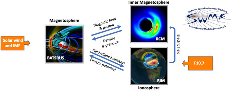
FIGURE 1. The SWMF Geospace model setup. The arrays indicate the one-way or two-way couplings between the modules (see text). The orange boxes indicate model input parameters.
BATSRUS, configured to solve the semi-relativistic MHD equations, models the solar wind and the magnetosphere with an adaptive grid resolution ranging from 0.125 RE in the near-Earth region to 8RE in the distant tail. The simulation box covers the region from 32 RE to −224 RE in the X direction and ±128 RE in the Y and Z directions in Geocentric Solar Magnetospheric (GSM) coordinates. The inner boundary is a spherical surface at radial distance R = 2.5 RE. The Geospace setup uses the ideal MHD equations to describe the large-scale plasma dynamics in the solar wind and magnetosphere. The adaptive grid is fixed in time, selected to focus the highest resolution to close to the dayside boundaries and to the magnetotail where many of the smaller scale dynamic processes take place.
The Ridley Ionosphere electrodynamics Model (RIM) solves the Poisson equation for the electrostatic potential on a two-dimensional height-integrated ionospheric surface (Ridley et al., 2004). BATSRUS passes field-aligned currents from the simulation inner boundary to RIM, which uses them to derive the ionospheric conductance distribution in combination with the background conductances from the solar illumination characterized with the F10.7 index. RIM solves the Vasyliunas equation (Vasyliunas and McCormack, 1970) for the electric potential, and feeds the electric field back to BATSRUS to drive the inner boundary condition for the plasma velocity. RIM and BATSRUS are coupled at every 5 s.
The non-Maxwellian plasmas in the inner magnetosphere are modeled by the Rice Convection Model (RCM) that solves the bounce- and pitch-angle-averaged phase space densities for protons, singly charged oxygen, and electrons (Toffoletto et al., 2003). BATSRUS feeds the outer boundary condition and magnetic field configuration and RIM feeds the E×B drift speed to RCM. The RCM plasma density and pressure values are returned to BATSRUS, which relaxes MHD values towards the RCM values with a 20 s relaxation time (De Zeeuw et al., 2004). The 2-way coupling of BATSRUS with RCM and the one-way coupling of RIM to RCM are performed every 10 s.
This configuration can represent the dynamic response of the magnetosphere and ionosphere to the strong solar wind driving during geomagnetic storms. The RCM facilitates development of strong ring current (Liemohn M. W. et al., 2018), and the ground magnetic disturbances can be computed by Biot-Savart integration of the currents external to the Earth, using both the MHD and RIM domains (Yu and Ridley, 2008).
The Geospace model takes the solar wind plasma parameters (density, temperature, velocity, magnetic field), the F10.7 radio flux, and the dipole orientation as function of time as input and boundary conditions, and develops the magnetosphere from an empty dipole subjected to the observed solar wind which is fed in to the Sunward boundary of the simulation box.
The SWMF and the Geospace configuration numerical schemes are described in detail in (Tóth et al., 2012; Pulkkinen et al., 2013; Gombosi et al., 2021).
We study a set of 131 geomagnetic storms with Dst minima below −50 nT identified from the time period 2010–2019 (Al Shidi et al., 2022, see Table 1). Each of the storms was run with the SWMF Geospace model described above, using the same model setup apart from the initial and boundary conditions given by the solar wind parameters and the F10.7 solar flux. The model outputs comprised the geomagnetic indices as well as noon-midnight and equatorial plane cuts of the 3D magnetosphere domain. Each of the storms was run from 6 h prior to onset for 54 h. While the ionospheric and geomagnetic index data was stored at 1-min intervals, the 2D magnetospheric output was saved at 15-min cadence.
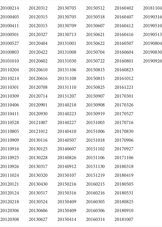
TABLE 1. Storm onset dates for events used in this study. For more detailed documentation see (Al Shidi et al., 2022) and the data availability statement.
Figures 2–4 show results from a sample storm that took place on March 16–17, 2015, and introduce the type of simulation results used in the following analysis. Figure 2 shows simulation results in the noon-midnight meridian plane with magnetopause identifications overlaid (see below).
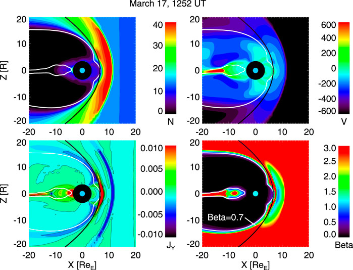
FIGURE 2. Noon-midnight meridian cuts from the simulation. (Top left) Plasma density in cm−3; (Top right) Plasma velocity VX component in km/s; (Bottom left) Current density in μA/m2; and (Bottom right) β* parameter (see text). The white lines show the β* = 0.7 contours, which are used to define the simulation magnetopause location. The black thick curve shows the Shue magnetopause model (see text).
Figure 3 shows the observed solar wind and IMF parameters as well as the geomagnetic indices compared with the simulation results shown in light blue. The storm main and recovery phases are indicated by the darker and lighter gray shading, respectively. The storm main phase is driven by strongly southward IMF as well as high-speed solar wind. The polar cap potential was of the order of 150 kV during the main phase, and the observed AL index reached below −1500 nT. Characteristically to the SWMF Geospace simulation, the simulation AL does not reach such low values. However, the bottom panel shows the Dst index, which is highly correlated with that derived from the simulation.
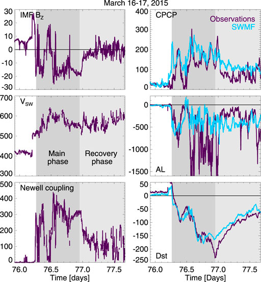
FIGURE 3. (Left panel) Solar wind driver parameters: (Top) IMF BZ in nT; (Middle) solar wind speed in km/s; and (Bottom) Newell coupling function (arbitrary units, see text). (Right panel) Geomagnetic index response: (Top) Cross-polar cap potential in kV; (Middle) Auroral electrojet AL index in nT; and (Bottom) Storm Dst index in nT. The observed valueas are shown in dark blue, the SWMF simulation values in light blue. Storm main phase (from start of Dst decrease to peak Dst) and recovery phase (from peak Dst to storm end) are shown with darker and lighter gray shading, respectively.
The left panels of Figure 4 show the magnetospheric tail magnetic field, electric current, and plasma velocity along the tail current sheet center in the midnight meridian in a keogram format. The higher values of the magnetic field in the magnetotail are characteristics of tail field dipolarizations. The strong current in the inner tail represents the intensifying ring current during the storm main phase. The flow speed shows both tailward and Earthward flow periods–here it is especially important to remember that the noon-midnight meridian represents only one location in the tail, while the flows are highly structured in the cross-tail dimension.
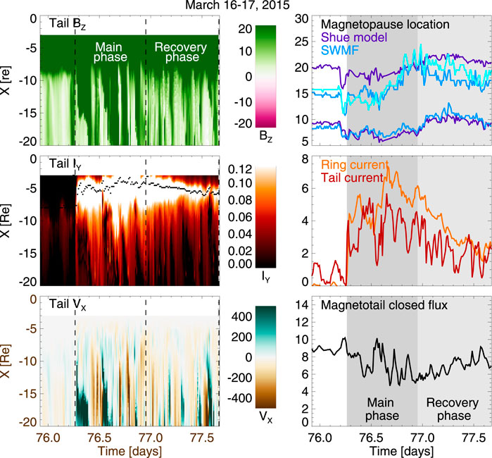
FIGURE 4. (Left panel) Simulation results along the magnetotail current sheet at the midnight meridian in a keogram format (see text for definition of the current sheet surface): (Top) Tail BZ in nT; (Middle) Z-integrated current intensity (arbitrary units, see text) with current peak intensity location shown with the black dotted line; (Bottom) Plasma velocity VX component in km/s. The storm main phase and recovery phases are defined by the dotted lines. (Right panel) Characteristic numbers for the magnetospheric state: (Top) Magnetopause nose at Y = Z = 0 and magnetopause distance from the X-axis at Y = 0, X = −10RE. The Shue model is shown in dark blue, the SWMF Geospace values are shown in lighter blue. The southern lobe simulation value is shown with the lightest shade of blue; the Shue model is symmetric and gives the same value for northern and southern lobes. (Middle) Total ring current (orange) and tail current (dark red) integrated along the tail length in MA (see text); (Bottom) Closed magnetic flux through the magnetotail at midnight meridian (arbitrary units, see text). Storm main phase (from onset to peak Dst) and recovery phase (from peak Dst to storm end) are shown with darker and lighter gray shading, respectively.
The right panels show the magnetopause locations, ring and tail current intensities, and the integrated magnetotail flux. Note the compression of the magnetospheric size during the storm main phase, and the high level of correlation between the tail and ring currents. More detailed description of each of the parameters will be provided in later sections.
For each storm, we identified onset time as the time when the Dst index starts to decrease (i.e., not necessarily the time of impact of an interplanetary coronal mass ejection or ICME), a storm peak as the time of the Dst minimum, and an end indicating recovery of the Dst index, a second major depression of the Dst index indicating another period of main phase -like activity, or end of simulation period. Note that while we wish to exclude main phase -like behavior from the analysis of recovery phase phenomena, we recognize that individual storms can have complex structure with multiple activations. Note also that many of the simulations do not reach to the end of the observed recovery phase. Furthermore, storms were categorized into two groups, “major storms” with peak Dst below −100 nT and “minor storms” with Dst peak between −50 and −100 nT, following often-used convention.
The full set of storms is represented in the form of a superposed epoch analysis. Figure 5 shows superposed epoch curves for the major (in red) and minor (in blue) storms with the standard deviation (orange/light blue shading) indicating the variability in each category. The superposition was done aligning the onset times, but time is not scaled to account for the main phase duration. The top row shows the ring current (Dst) index, the middle row the auroral electrojet (AL) index, and the bottom row shows the cross-polar cap potential (CPCP) from the northern hemisphere. The left column shows the observed indices extracted from the OMNI database (htpps://omniweb.nasa.gov); the CPCP values are computed using the formulation from (Ridley et al., 2004) as a function of the polar cap index (PCI) measured in the northern polar cap (Thule station) and season as
where the time of year is scaled as T = 2π(NMONTH/12) and the numbering of months starts from zero (Jan = 0). The middle column shows the simulated values, while the right column show the difference between the simulated and observed values, i.e., the model error and its variance.
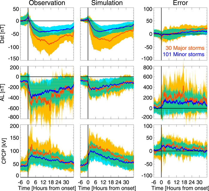
FIGURE 5. (Top row) Dst; (Middle row) AL; and (Bottom row) CPCP from (Left column) Observations; (Middle column) Simulation; and (Right column) Error (simulation–observation) for minor (blue, peak Dst
The simulations of the major and minor storms give quite good prediction of the Dst index, with relatively moderate errors between the model and observed values. The errors are closest to zero during the storm start and main phase, while they systematically increase (more for the major storms) during the recovery phase. This indicates that the Geospace model has a tendency to predict smaller Dst disturbance during the recovery phase, i.e., recover faster than the observed Dst.
The AL index has large variability in observations, while the values and the variability are much smaller in the simulation. Consequently, the errors are large with no systematic trend during the storm for minor storms, but a tendency for larger errors during the storm main phase than during the recovery phase for major storms. For strong AL activity, the Geospace model AL indices are substantially weaker than the observed ones. Furthermore, as accurate modeling of individual substorms still poses a major challenge to the simulations, the timing differences in the substorm evolution cause large instantaneous errors in the observed and model values.
The simulated polar cap potentials are somewhat larger than those obtained from the empirical model, and furthermore show a larger difference between the averages of the major and minor storms. The errors are largest during the main phase, while close to zero during the recovery phase. This means that the simulation predicts larger polar cap potentials than the empirical model, indicative of either stronger dayside merging or weaker tail reconnection during the storm main phase.
The model performance can be assessed by computing skill scores for the geomagnetic index predictions. The Heidke skill score (Heidke, 1926) is one often used performance measure for geomagnetic index predictions, and is defined as
where H = hit, M = miss, F = false positive, and N = true negative, which are evaluated based on the observation and prediction values being above or below the selected thresholds. The HSS maximum value for no misses and no false positives is 1, value of zero indicates no skill, and negative values indicate skill worse than chance coincidence.
Figure 6 shows heat map plots of hourly averaged index values for Dst, AL, and the polar cap potential, as well as the errors as function of the observed index values (right column). The left and middle column show the major and minor storms separately. The dotted lines indicate the chosen “event” values for the Heidke skill score calculation (−50 nT for Dst, − 150 nT for AL, and 80 kV for the CPCP). While changing the selected “event” values somewhat changes the skill scores, our conclusions are independent of the exact values of the limits.
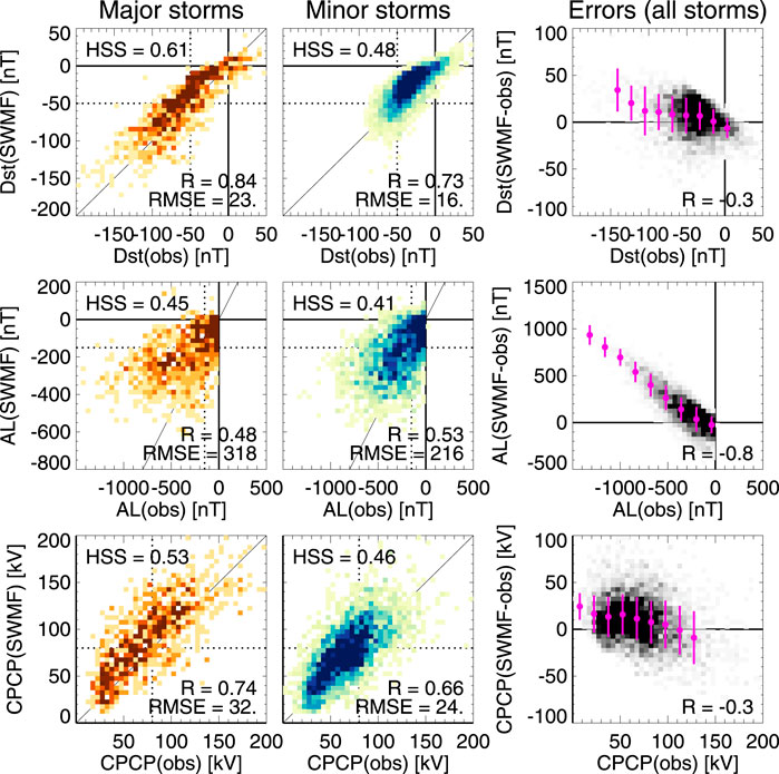
FIGURE 6. Heat map plots showing hourly values of (Top row) Dst; (Middle row) AL; and (Bottom row) the CPCP observed vs. simulated values, for (Right column) major storms and(Center column) minor storms. The unity line is shown in thin solid line, the dotted linesshow the threshold values used in the Heidke Skill Score (HSS) calculation (see text).The heat maps indicate the share of points falling in each bin. (Right column) Errors(simulated -- observed value) as function of the observed values. The magenta dotsshow bin averages, and the vertical thin lines indicate the standard deviation in eachbin.
The Heidke skill score for the major storms is HSS = 0.61, which is somewhat better than the value 0.57 obtained by (Liemohn M. W. et al., 2018), who computed skill scores for a 3-month period including both storm and nonstorm times. The skill for the smaller storms is lower (0.48). Furthermore, the skill scores for the AL and the CPCP are lower, showing similar difference between major and minor storms. Comparison between minor and major storms and with the Liemohn et al. (2018) results indicate that the Heidke skill scores are larger for data sets that contain sufficient number of data points in the “hit” quadrant.
The plots also indicate the values of the commonly used Pearson linear correlation coefficient defined as the ratio of the covariance and the product of the standard deviations of each set (o = observation, m = model:
where the covariance is given by ∑i (mi − < m >) (oi − < o >)/(N − 1) and the variance (square of the standard deviation) is given by
The right column shows the errors (simulation–observation) as function of the observed values. All errors show a tendency to increase with increasing level of activity, but for Dst and CPCP, the effect is relatively minor. On the other hand, the error in AL is strongly and almost linearly dependent on the intensity of the AL index throughout the higher values of the observed AL. This indicates that the simulation value is smaller than the predicted value by a factor dependent on the intensity of the (observed) activity. While the scatter in the values is still large, the model predictive performance could be improved by accounting for this persistent behavior.
Most geomagnetic activity predictions rely on empirical relationship between the driving solar wind and interplanetary magnetic field and the resulting geomagnetic activity. The Newell coupling function (Newell et al., 2007), representing the rate of change of magnetic flux at the nose of the magnetopause, is given by
where θ = tan−1(BY/BZ) is the IMF clock angle and
Figure 7 shows the geomagnetic indices as function of the Newell coupling function separately for the main phase and recovery phases for all storms. The data are averaged to 1-h bins, which should remove most scatter associated with timing errors of the arrival time of the solar wind front at the subsolar bow shock. Correlations are shown both for observations (dark purple) and simulation results (magenta). The correlations don’t show significant differences between the main and recovery phases, but the scatter during the recovery phase is somewhat smaller.
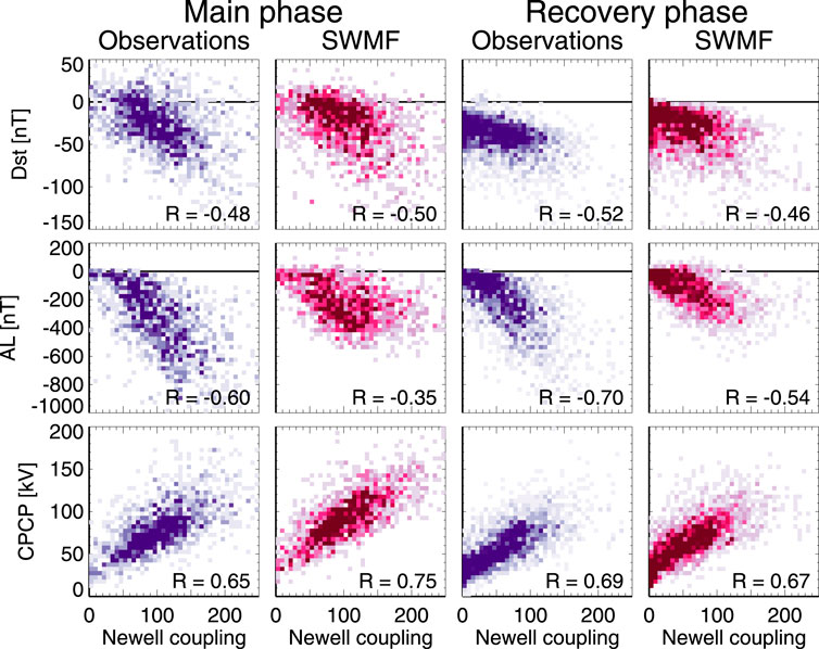
FIGURE 7. (Top row) Dst; (Middle row) AL; and (Bottom row) CPCP during (Left two columns) the storm main phase and (Right two columns) recovery phase as function of the Newellcoupling function (in arbitrary units) using 1-hour averaged data for observations (darkpurple) and simulations (dark red). The heat maps indicate the share of points falling ineach bin.
Essentially, the distribution of points for the observations and the simulation look similar. This indicates that the simulation is doing as good a job in the prediction as the observations. On the other hand, despite the simulation being deterministic, it does not provide better correlations. This fact emphasizes that better observations will not lead to improved correlations (as the simulation can use data from any point), and that improving the predictions requires better coupling functions (with inclusion of time history of the solar wind driver and magnetospheric state).
Using two-dimensional cuts in the simulation saved at 15-min cadence, we examine the properties at the center of the current sheet along the midnight meridian. The current sheet center is defined as the point with minimum BX between the lobes for each X-value along the tail, which in a simple geometry coincides with the peak of the current intensity. At times, the current sheet is bifurcated tailward of a large-scale neutral line. In such cases, the algorithm chooses one or the other branches and uses those values as the current sheet center. This choice does not significantly impact our results that focus on the inner magnetosphere.
For each storm and each time step, we identify the current sheet center location ZCS along the midnight meridian, plasma velocity VX, magnetic field BZ, and current jY at the current sheet center, and integrate the total current (JY(X) = ∫jYdZ) across the current sheet thickness. We extend the analysis out to X = −20RE.
Furthermore, we identify the location of the innermost X-line, XNL, from a BZ sign change, and calculate the amount of closed magnetic flux through the tail from
where the limit at − 3RE is close to the inner boundary of the simulation domain. As the analysis is limited to X > − 20RE, for situations where the X-line is further than that, we set XNL = −20RE (the flux crossing the equatorial plane beyond that distance is small and would not cause significant changes to the results). Furthermore, as the magnetic flux is generally defined as magnetic field through an area, and we are limited here to the two-dimensional noon-midnight plane (i.e. flux per unit cross-tail width), we show the closed flux in arbitrary units focusing on time variations rather than absolute values.
While the distinction between tail and ring current is arbitrary as well in observations as in the simulation, we denote the current inside of 8 RE as the “ring current” and the current tailward of 8 RE as “tail current”. Similarly to the magnetic flux, we integrate the total ring and tail currents crossing the midnight meridian as
Figure 8 shows the relationship of the ring current, tail current, and closed flux with the Dst index and the cross-polar cap potential. The good correlation between the ring current and the Dst index shows that, indeed, the Dst index is a good (albeit not strictly linear) measure of the ring current. The ring current intensity for the same value of Dst is higher during the main phase than during the recovery phase, which likely comes from the positive contribution to Dst from the dayside compression, which is often larger during the main phase than during the recovery phase. The amount of closed flux along the midnight meridian is likewise well correlated with Dst, linking the decrease of tail magnetic flux to the intensification of the ring (and tail) currents.
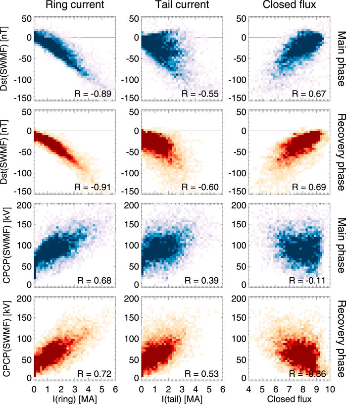
FIGURE 8. (Top two rows) Dst and (Bottom two rows) CPCP from the SWMF simulation as function of (Left column) total ring current; (Middle column) total tail current; and (Right column) Closed magnetic flux in the tail (see definitions given in the text). The storm main phase (blue) and recovery phase (orange) are shown separately. The data are snapshotstaken at 15-min cadence in the magnetotail, tagged with the 30-min smoothed values ofthe indices. The heat maps indicate the share of points falling in each bin.
The tail current shows a larger variability, but still clear correlation with the Dst index, indicating that the currents even beyond − 8RE contribute to the index in a significant way.
As the polar cap potential is quite directly driven by the changing solar wind driver, correlations with the CPCP indicate directly driven processes. It is evident that the ring current is more directly driven (i.e. has better correlation with the CPCP than the tail current, or the closed magnetic flux, that shows very low if any correlation with the polar cap potential).
Figure 9 shows the ring current and the Dst index from the simulation as functions of the Newell coupling parameter. The coupling parameter was smoothed by a 30-min filter before tagging the values to the simulation values. If the coupling parameter were a perfect indicator of the state of the magnetosphere, one would expect a very high correlation, as the simulation itself is a self-consistent, fully deterministic system. If the coupling function is not a perfect predictor of the ring current, there are other factors than those included in the coupling function that affect the state of the ring current. As can be seen in the figure, the scatter in these parameters is large, indicative of the complexity of the processes and the significance of prior history both of the driver and of the magnetospheric dynamics not included in a point-by-point correlations. This complexity of course reflects on the scatter between the driver function and the geomagnetic indices discussed above. This conclusion remains valid even if we acknowledge that the simulation is not a perfect model of the true magnetospheric plasma system.
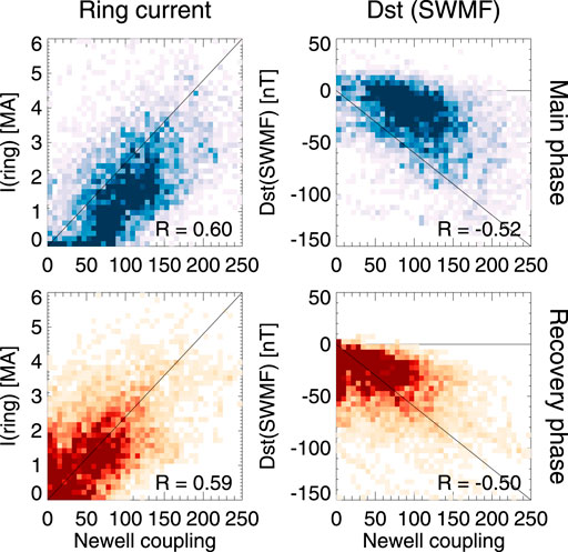
FIGURE 9. (Left) Total ring current and (Right) the simulation Dst during the main phase (top row) and recovery phase (bottom row) as function of Newell coupling function (in arbitrary units). The data are snapshots taken at 15-min cadence in the magnetotail, tagged with the 30-min smoothed values of the driver intensity. The heat maps indicate the share ofpoints falling in each bin.
The coupling function comparison between the storm main and recovery phases is an indicator of the effects of time history to the correlations. The ring current intensity for similar level of driving is slightly higher for the recovery phase (likely indicating a higher preceding values of the current). Comparing to the Dst index, the difference is even more significant, highlighting the effects of the dayside processes on the Dst index. For the closed flux and cross-polar potential there is no difference in the distributions during storm main and recovery phases (not shown).
The size of the magnetosphere is often characterized by the subsolar magnetopause location, which together with the flaring angle describes the shape of the boundary in the downwind direction. Statistical analyses yielded an empirical relationship (Shue et al., 1997), revised for extreme periods (Shue et al., 1998) to the form
The subsolar magnetopause nose distance from the Earth R0 is given in RE when the IMF BZ is given in nT and the solar wind pressure P in nPa. The model assumes cylindrical symmetry, and produces a flaring magnetotail with the degree of flaring controlled by the factor α dependent on both IMF BZ and dynamic pressure P.
We determined the magnetopause location from the 2D simulation cuts in the noon-midnight meridian plane using the open-closed field line boundary (in the dayside) and a parameter β* = 2μ0(Pth + P)/B2, which on the nightside shows a clear boundary between the dense magnetosheath with high β* > 1 and the low-density, high-field magnetotail lobe with low β* ≪ 1 (see bottom left panel of Figure 2; Brenner et al., 2021). In determining the boundary location, we used a limit value of β* = 0.7, but changing the limit value causes minimal changes to the outcome. Figure 2 shows the magnetopause definition overlaid with other parameters. This definition agrees with a velocity shear region at the high latitude tail magnetopause as well as follows closely the peak magnetopause currents.
Figure 2 also shows how the two magnetopause definitions agree during the storm main phase: The subsolar locations are close to each other, but the Shue model flares much more than the magnetopause defined using the β* parameter in the simulation. This is true more generally beyond the individual time step shown here: Figure 4 shows time series for the subsolar point location as well as two individual points at X = −10RE at the northern and southern tail lobes. While the subsolar locations agree for most of the time, the magnetotail size in the SWMF is smaller than that predicted by the Shue model throughout the storm with the exception of a short interval near the end of the main phase of the storm. Note also that the simulation magnetopause has a lot of small-scale variability, which is not always symmetric between the northern and southern lobes, indicating that the internal magnetospheric dynamics and the changing dipole tilt angle also contribute to the shape of the magnetopause.
Figure 10 shows a statistical comparison of the subsolar and high-latitude (Y = 0, X = −10RE) tail magnetopause locations identified from the Geospace simulation and obtained from the Shue model using the formulation above. While there is a general correlation, there are clear deviations between the models.
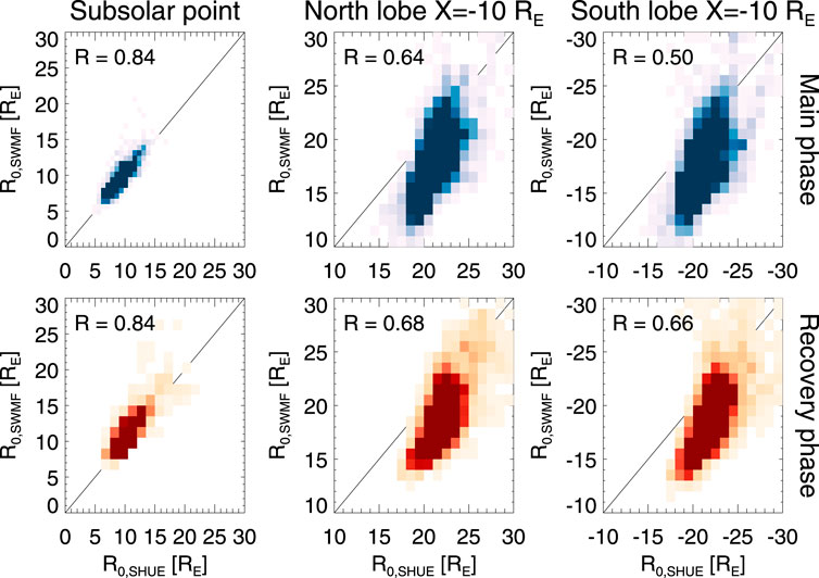
FIGURE 10. SWMF magnetopause location vs. the Shue model. (Left) Magnetopause subsolarposition X-value for Y = Z = 0. (Middle) North lobe magnetopause position Z-value at Y = 0, X = -10 RE. (Right) South lobe magnetopause position Z-value at Y = 0, X=-10 RE. (Top row) storm main phase, (Bottom row) storm recovery phase. The heat maps indicate the share of points falling in each bin.
For the subsolar point, the models agree very well. However, generally the SWMF magnetopause values are slightly larger than the Shue model values. There are a few isolated occurrences where the SWMF values are considerably higher than those predicted by the Shue model. All of those occur during periods of very low solar wind density and moderate solar wind speed combined with negative IMF BZ, and low Alfvén Mach numbers
The center and right panels show the magnetopause position at Y = 0, X = −10RE. At the high-latitude magnetotail, the magnetopause in SWMF is typically much closer to the Sun-Earth line than the Shue model for strongly driven conditions (smallest sizes of the magnetosphere). For more average driving conditions (and during the storm recovery phase), the difference diminishes, but the majority of Shue model values still fall below the Geospace ones.
Lastly we examine the magnetopause location dependence on the IMF driver parameters. Figure 11 shows the subsolar and north tail lobe locations as function of solar wind dynamic pressure and IMF BZ component. The black curves show the functional dependence of the Shue model (proportional to P−1/6.6) to guide the eye (not a fit to the points). It is clear that the functional dependence for the subsolar location is similar for both the Shue model and the SWMF Geospace results, as the distributions almost completely overlap. However, for the tail lobe location, the functional form seems to still be valid for the SWMF results (with large scatter), but the flaring angle formula, which also includes dynamic pressure, changes that for the Shue model. Thus, the solar wind dynamic pressure response of the simulation differs from that given by the Shue formulation, leading to less flaring tail and smaller tail lobe cross-sectional area.
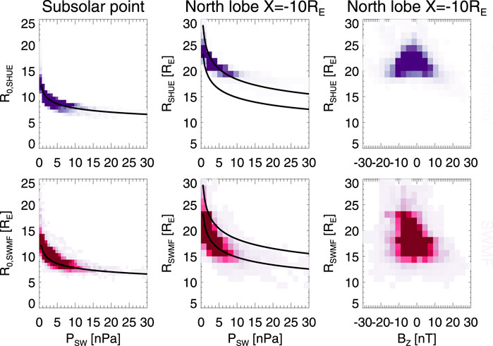
FIGURE 11. Magnetopause location vs solar wind driver parameters during the storm main phase. (Left) Magnetopause subsolar position X-value for Y = Z = 0 as function of solar wind dynamic pressure. (Middle) North lobe magnetopause position Z-value at Y = 0, X = -10 RE as function of solar wind dynamic pressure. (Right) North lobe magnetopause position Z-value at Y = 0, X = -10 RE as function of IMF BZ. (Top row) The Shue model values are shown in blue, (Bottom row) the SWMF values are shown in red. The black lines show the Shue model functional dependence on dynamic pressure (P{-1/6.6}) using arbitrary scaling.
The right panel of Figure 11 showing the tail lobe magnetopause dependence on the IMF BZ documents that the magnetopause dependence on that parameter is at best weak. The largest magnetopause distances (largest flaring) is obtained when BZ is close to zero, while both highly negative and highly positive IMF BZ lead to compressed magnetosphere–much more so for the SWMF than for the Shue model.
In this paper, we show results from the first large-scale statistical set of geomagnetic storm simulations developed by Al Shidi et al. (2022). We focus especially on comparing the geomagnetic indices with observed values as well as their dependence on the solar wind driver functions. While we did not have sufficient storage space to store all 3D simulation data, we focus on the 2D noon-midnight plane cuts and examine the magnetotail parameters along the tail current sheet center as well as the magnetopause locations at the dayside and in the magnetotail.
The statistical results can be used to infer the characteristic behavior of the SWMF Geospace simulation in a quantitative manner. All the examined indices (Dst, AL, CPCP) show behavior that is different during the storm main phase and recovery phase: For Dst, the error (simulated–observed value) is smallest during the main phase and increases systematically toward the recovery phase, while the opposite is true for the AL and CPCP. Thus, the model Dst index recovers faster than the observed one, indicating that further modeling or parametrization of the ring current decay processes could improve the model performance. Such processes could either be related to charge exchange and Coulomb collisions (Dessler and Parker, 1959; Fok et al., 1995) the wave-particle interactions scattering the ions away from the ring current (Jordanova et al., 2001; Yue et al., 2019), multi-ion physics (Daglis, 2006) or ion outflow from the ionosphere (Glocer et al., 2012). Regarding model performance metrics, the results in this paper, focusing solely on storm periods, are slightly better in terms of the HSS than those obtained by (Liemohn M. et al., 2018), who used 3 months of real-time simulation containing both quiet and storm periods, but dominated by quiet periods.
The AL index shows a consistent offset from the observed value, which calls for further investigation of the auroral electrodynamics and magnetosphere–ionosphere coupling processes, including the acceleration region processes (Liemohn et al., 2002; Connor et al., 2016). Especially, the model has poor capability to reproduce the largest AL values, with the simulated values mostly limited to above −800 nT; the same is true for comparison with local magnetic perturbations (Al Shidi et al., 2022). Furthermore, the instantaneous values of the AL index are critically dependent on timing of the substorm onsets and hence magnetotail dynamic processes, which still are difficult to reproduce to high accuracy in location and timing (Newell et al., 2016; Maimaiti et al., 2019).
The auroral conductances regulate the closure of the field-aligned currents through the Hall and Pedersen currents in the ionosphere (Iijima and Potemra, 1976; Ridley et al., 2004). In general, auroral conductance arises from the solar EUV radiation in the dayside and from energetic particle precipitation to the auroral oval region especially in the nightside (Fuller-Rowell and Evans, 1987; Newell et al., 2009). In the SWMF simulation, the auroral conductances are derived from a simple empirical parametrization, which may in part lead to weaker coupling of the magnetotail currents into the ionosphere. Mukhopadhyay et al. (2020) examined the conductance effects on the coupling, and propose a new model for the auroral conductances, which has been coupled to the SWMF simulation. The CMEE model for auroral conductances allows for a larger range of values, which lead to lower cross-polar potential values (as a result of currents closing between R1 and R2 currents), and larger ground magnetic perturbation values (Mukhopadhyay et al., 2020). However, accurate modeling of both the diffuse and discrete sources and inclusion of their ionospheric impacts into the global simulations is still work in progress (Mukhopadhyay et al., 2022).
The polar cap potential is a central parameter describing the balance between dayside and nightside energy conversion processes, but observationally we are limited to radar (model-based) estimates of the convection (Koustov et al., 2009; Gao, 2012), low-Earth orbit satellite electric field measurements (Hairston et al., 1998), or empirical models based on the polar cap index (Troshichev et al., 1996; Ridley et al., 2004). The Ridley epirical model (Ridley et al., 2004) has quite high correlation with the simulated polar cap potential time series, with the simulation producing slightly higher potentials especially during the storm main phase. The Ridley model based on the PCI is quite directly driven by the solar wind and IMF parameters, as is the simulation polar cap potential. Better global observations of the CPCP evolution are needed to fully understand the role of the detailed magnetospheric processes on the polar cap potential evolution.
The anticorrelation of the errors between the polar cap potential and the AL index indicates that the current closure processes between the ionosphere and the magnetosphere could be further optimized in the simulation. It seems that sometimes the magnetotail reconnection is not sufficiently strong to balance the dayside energy input, leading to weaker auroral currents (and hence AL) and stronger polar cap potential (larger lobe flux) (Milan et al., 2003; Lockwood et al., 2009).
An important part of empirical predictions of the magnetospheric and ionospheric states is the use of coupling functions that tie the solar wind parameters to their geomagnetic response. For example, assuming that a solar wind coupling function is able to predict the ring current intensity, a deterministic simulation should always yield a good correlation. On the other hand, data contain many uncertainties: the solar wind input from L1 may be different than that impacting the Earth, and the Dst index is an indirect measure of the true ring current and may miss localized signatures. Therefore, even for a perfect coupling parameter, one would expect to have scatter in the results. Our results show that the distributions of the deterministic model and the observations are similar. This indicates that the scatter in the results arises largely from the inability of the simple coupling parameter to represent the complex solar wind–magnetosphere coupling and its time history, and that their predictive power cannot be further increased with a denser observational network. The magnetospheric processes as well as the time history of the system have quite strong effects on the system response, which yield high level of scatter in the correlation figures (see Figure 7, (Tsyganenko and Sitnov, 2005)). It also points out to the usefulness of a physics-based model over a prediction based on solar wind input only.
Analysis of the nightside ring current and tail current intensities shows that the ring current is highly correlated with the Dst index, but that there is a difference between the storm main and recovery phases. This likely stems from the dayside positive contribution to the Dst index, which is higher during the main phase. It is also noteworthy that the tail current and ring current intensities are highly correlated, and that they are of almost equal magnitude during the storm main phase, while the ring current starts to dominate during later phases of the storm, consistent with earlier observational and empirical model studies (Ganushkina et al., 2005; Kalegaev and Makarenkov, 2008). In our study, the “ring current” was arbitrarily defined as the current inside 8 RE, which is the domain covered by the RCM drift physics model, while the “tail current” was taken to be everything tailward of that. The results are not sensitive to the exact separation distance.
The subsolar distance to the magnetopause is largely determined by the solar wind dynamic pressure, but the orientation and magnitude of the IMF, the time history of the solar wind, as well as internal state of the magnetosphere cause substantial scatter to the results. The Geospace model gives quite good agreement with the empirical (Shue et al., 1998) model developed using a statistical database of magnetopause crossings, but the results along the magnetopause flank vary quite a bit from the empirical paraboloid shape. Especially during highly compressed situations (high dynamic pressure), the Geospace simulation gives significantly smaller distances from the Sun-Earth line to the lobe boundary than the empirical model.
Shukhtina et al. (2004) derived the magnetopause location using both solar wind parameters and tail magnetic flux derived from the Geoatail measurements, parametrizing the tail flaring angle. They demonstrate the strong dependence of the size of the magnetosphere on the internal state of the magnetosphere, by examining quiet periods, periods close to substorm onset, and periods of steady magnetospheric convection, which are characterized by enhanced, steady-state convection in the magnetotail, an expanded polar cap and enhanced lobe magnetic flux content (Sergeev et al., 1996).
Gordeev et al. (2015) performed an extensive comparison of global MHD simulations of the Earth’s space environment using the Community Coordinated Modeling Center (CCMC) resources and four different MHD simulations, including BATSRUS, the MHD simulation core of the SWMF Geospace model used in this study. When comparing the results in that paper with our results, two things must be pointed out: (1) the Gordeev et al. (2015) study used the MHD simulations without coupling to an inner magnetosphere model, which significantly alters the “memory” of the magnetosphere, when the ring current response is not included, and (2) the comparison was made using an artificially created solar wind time series including constant solar wind and a constant IMF that flipped from BZ northward to BZ southward after 2 h of northward IMF. In our case, we have simulated real events, which involve all the complexities of true solar wind driver characteristics. The Gordeev et al. (2015) study shows that the pure BATSRUS gives a subsolar location that is very highly correlated with the Shue et al. (1998) model, with even higher correlation coefficient (0.95) than that found in this study, and BATSRUS was the best-performing simulation of the four examined in that metric. They also showed that BATSRUS produces good agreement with the Lin et al. (2010) model of the high-latitude magnetotail boundary. That model provides a more detailed description of the tail boundary including effects of the dipole tilt angle in addition to the solar wind and IMF parameters.
In conclusion, we show results from a first large statistical study of storm simulations using the SWMF Geospace model. The results help assess the usability of the geomagnetic indices, the solar wind driver functions, and point further to magnetotail parameters that could be used to define the state of the magnetosphere.
The datasets analyzed for this study can be found in the University of Michigan Deep Blue repository under: Al Shidi et al. (2022). Space Weather Modeling Framework simulations of ground magnetometer data [Data set], University of Michigan - Deep Blue Data. DOI: https://doi.org/10.7302/dkjd-1j05 under Creative Commons license http://creativecommons.org/licenses/by/4.0/.
TP did the analysis and wrote majority of the analysis. AB developed the methods and helped analyze the 2D data. QA developed methods and helped analyze the geomagnetic index data. GT advised on the use of the Geospace simulation.
NSF grant 2033563 supported analysis of the storm simulation results on solar wind entry into the magnetosphere and developing the analysis methodology. NASA grant 80NSSC21K1753 supported running the simulations and analysis of the results.
The authors declare that the research was conducted in the absence of any commercial or financial relationships that could be construed as a potential conflict of interest.
All claims expressed in this article are solely those of the authors and do not necessarily represent those of their affiliated organizations, or those of the publisher, the editors and the reviewers. Any product that may be evaluated in this article, or claim that may be made by its manufacturer, is not guaranteed or endorsed by the publisher.
Akasofu, S.-I. (1981). Energy coupling between the solar wind and the magnetosphere. Space Sci. Rev. 28, 121–190. doi:10.1007/bf00218810
Al Shidi, Q., Pulkkinen, T. I., Brenner, A., Toth, G., and Gjerloev, J. (2022). Can simulations predict ground magnetic perturbations? Space Weather. submitted.
Axford, W. I., and Hines, C. O. (1961). A unifying theory of high-latitude geophysical phenomena and geomagnetic storms. Can. J. Phys. 39, 1433–1464. doi:10.1139/p61-172
Borovsky, J. E., and Birn, J. (2014). The solar wind electric field does not control the dayside reconnection rate. J. Geophys. Res. Space Phys. 119, 751–760. doi:10.1002/2013JA019193
Brenner, A., Pulkkinen, T. I., Al Shidi, Q., and Toth, G. (2021). Stormtime energetics: Energy transport across the magnetopause in a global MHD simulation. Front. Astron. Space Sci. 8, 180. doi:10.3389/fspas.2021.756732
Burton, R. K., McPherron, R. L., and Russell, C. T. (1975). An empirical relationship between interplanetary conditions and Dst. J. Geophys. Res. 80, 4204–4214. doi:10.1029/ja080i031p04204
Connor, H. K., Zesta, E., Fedrizzi, M., Shi, Y., Raeder, J., Codrescu, M. V., et al. (2016). Modeling the ionosphere-thermosphere response to a geomagnetic storm using physics-based magnetospheric energy input: OpenGGCM-CTIM results. J. Space Weather Space Clim. 6, A25. doi:10.1051/swsc/2016019
Crooker, N. U. (1988). Mapping the merging potential from the magnetopause to the ionosphere through the dayside cusp. J. Geophys. Res. 93, 7338–7344. doi:10.1029/JA093iA07p07338
Daglis, I. A. (2006). Ring current dynamics. Space Sci. Rev. 124, 183–202. doi:10.1007/s11214-006-9104-z
Davis, T. N., and Sugiura, M. (1966). Auroral electrojet activity index AE and its universal time variations. J. Geophys. Res. 71, 785–801. doi:10.1029/JZ071i003p00785
De Zeeuw, D., Sazykin, S., Wolf, R., Gombosi, T., Ridley, A., and Tóth, G. (2004). Coupling of a global MHD code and an inner magnetospheric model: Initial results. J. Geophys. Res. 109, A12219. doi:10.1029/2003JA010366
Dessler, A. J., and Parker, E. N. (1959). Hydromagnetic theory of geomagnetic storms. J. Geophys. Res. 64, 2239–2252. doi:10.1029/jz064i012p02239
Fok, M., Moore, T. E., Kozyra, J. U., Ho, G. C., and Hamilton, D. C. (1995). Three-dimensional ring current decay model. J. Geophys. Res. 100, 9619. doi:10.1029/94ja03029
Fuller-Rowell, T. J., and Evans, D. S. (1987). Height-integrated Pedersen and Hall conductivity patterns inferred from the TIROS-NOAA satellite data. J. Geophys. Res. 92, 7606–7618. doi:10.1029/ja092ia07p07606
Ganushkina, N. Y., Pulkkinen, T. I., and Fritz, T. (2005). Role of substorm-associated impulsive electric fields in the ring current development during storms. Ann. Geophys. 23, 579–591. doi:10.5194/angeo-23-579-2005
Gao, Y. (2012). Comparing the cross polar cap potentials measured by SuperDARN and AMIE during saturation intervals. J. Geophys. Res. 117, A08325. doi:10.1029/2012JA017690
Glocer, A., Kitamura, N., Tóth, G., and Gombosi, T. (2012). Modeling solar zenith angle effects on the polar wind. J. Geophys. Res. 117. doi:10.1029/2011JA017136
Gombosi, T. I., Chen, Y., Glocer, A., Huang, Z., Jia, X., Liemohn, M. W., et al. (2021). What sustained multi-disciplinary research can achieve: The space weather modeling framework. J. Space Weather Space Clim. 11, 42. doi:10.1051/swsc/2021020
Gonzalez, W. D., Joselyn, J. A., Kamide, Y., Kroehl, H. W., Rostoker, G., Tsurutani, B. T., et al. (1994). What is a geomagnetic storm? J. Geophys. Res. 99, 5771–5792. doi:10.1029/93ja02867
Gordeev, E., Sergeev, V., Honkonen, I., Kuznetsova, M., Rastätter, L., Palmroth, M., et al. (2015). Assessing the performance of community-available global mhd models using key system parameters and empirical relationships. Space Weather. 13, 868–884. doi:10.1002/2015sw001307
Hairston, M. R., Weimer, D. R., Heelis, R. A., and Rich, F. (1998). Analysis of the ionospheric cross polar cap potential drop and electrostatic potential distribution patterns during the January 1997 CME event using DMSP data. J. Atmos. Sol. Terr. Phys. 61, 195–206. doi:10.1016/s1364-6826(98)00128-x
Häkkinen, L. V. T., Pulkkinen, T. I., Nevanlinna, H., Pirjola, R. J., and Tanskanen, E. I. (2002). Effects of induced currents on dst and on magnetic variations at midlatitude stations. J. Geophys. Res. 107, 1014–SMP 7–8. doi:10.1029/2001JA900130
Heidke, P. (1926). Berechnung des erfolges und der gute der windstarkevorhersagen im sturmwarnungsdienst. Geogr. Ann. 8, 301–349. doi:10.2307/519729
Hu, Y.-Q., Guo, X.-C., Li, G.-Q., Wang, C., and Huang, Z.-H. (2005). Oscillation of quasi-steady Earth’s magnetosphere. Chin. Phys. Lett. 22, 2723–2726. doi:10.1088/0256-307X/22/10/073
Iijima, T., and Potemra, T. A. (1976). The amplitude distribution of field-aligned currents at northern high latitudes observed by Triad. J. Geophys. Res. 81, 2165–2174. doi:10.1029/ja081i013p02165
Janhunen, P., Palmroth, M., Laitinen, T., Honkonen, I., Juusola, L., Facskó, G., et al. (2012). The GUMICS-4 global MHD magnetosphere-ionosphere coupling simulation. J. Atmos. Solar-Terrest. Phys. 80, 48–59. doi:10.1016/j.jastp.2012.03.006
Jordanova, V. K., Farrugia, C. J., Thorne, R. M., Khazanov, G. V., Reeves, G. D., and Thomsen, M. F. (2001). Modeling ring current proton precipitation by electromagnetic ion cyclotron waves during the may 14–16, 1997, storm. J. Geophys. Res. 106, 7–22. doi:10.1029/2000JA002008
Kalegaev, V. V., and Makarenkov, E. V. (2008). Relative importance of ring and tail currents to Dst under extremely disturbed conditions. J. Atmos. Solar-Terrest. Phys. 70, 519–525. doi:10.1016/j.jastp.2007.08.029
Kilpua, E., Koskinen, H. E. J., and Pulkkinen, T. I. (2017). Coronal mass ejections and their sheath regions in interplanetary space. Living Rev. Sol. Phys. 14, 5. doi:10.1007/s41116-017-0009-6
Koustov, A. V., Khachikjan, G. Y., Makarevich, R. A., and Bryant, C. (2009). On the SuperDARN cross polar cap potential saturation effect. Ann. Geophys. 27, 3755–3764. doi:10.5194/angeo-27-3755-2009
Kwagala, N. K., Hesse, M., Moretto, T., Tenfjord, P., Norgren, C., Tóth, G., et al. (2020). Validating the space weather modeling framework (SWMF) for applications in northern europe. Ground magnetic perturbation validation. J. Space Weather Space Clim. 10, 33. doi:10.1051/swsc/2020034
Lakka, A., Pulkkinen, T. I., Dimmock, A. P., Myllys, M., Honkonen, I., and Palmroth, M. (2018). The cross-polar cap saturation in GUMICS-4 during high solar wind driving. J. Geophys. Res. Space Phys. 123, 3320–3332. doi:10.1002/2017JA025054
Liemohn, M. W., Kozyra, J. U., Clauer, C. R., Khazanov, G. V., and Thomsen, M. F. (2002). Adiabatic energization in the ring current and its relation to other source and loss terms. J. Geophys. Res. 107, 1045. doi:10.1029/2001JA000243
Liemohn, M., Ganushkina, N., De Zeeuw, D., Rastaetter, L., Kuznetsova, M., Welling, D., et al. (2018). Real-time swmf at ccmc: assessing the dst output from continuous operational simulations. Space Weather. 16, 1583–1603. doi:10.1029/2018SW001953
Liemohn, M. W., McCollough, J. P., Jordanova, V. K., Ngwira, C. M., Morley, S. K., Cid, C., et al. (2018). Model evaluation guidelines for geomagnetic index predictions. Space Weather. 16, 2079–2102. doi:10.1029/2018SW002067
Lin, R. L., Zhang, X. X., Liu, S. Q., Wang, Y. L., and Gong, J. C. (2010). A three-dimensional asymmetric magnetopause model. J. Geophys. Res. 115. doi:10.1029/2009JA014235
Lockwood, M., and McWilliams, K. A. (2021). On optimum solar wind-magnetosphere coupling functions for transpolar voltage and planetary geomagnetic activity. JGR. Space Phys. 126, e2021JA029946. doi:10.1029/2021ja029946
Lockwood, M., Hairston, M., Finch, I., and Rouillard, A. (2009). Transpolar voltage and polar cap flux during the substorm cycle and steady convection events. J. Geophys. Res. 114, A01210. doi:10.1029/2008JA013697
Lockwood, M. (2019). Does adding solar wind poynting flux improve the optimum solar wind-magnetosphere coupling function? JGR. Space Phys. 124, 5498–5515. doi:10.1029/2019JA026639
Lockwood, M. (2022). Solar wind—Magnetosphere coupling functions: Pitfalls, limitations, and applications. Space Weather. 20, e2021SW002989. doi:10.1029/2021sw002989
Lopez, R. E., Bruntz, R., Mitchell, E. J., Wiltberger, M., Lyon, J. G., and Merkin, V. G. (2010). Role of magnetosheath force balance in regulating the dayside reconnection potential. J. Geophys. Res. 115, 216. doi:10.1029/2009JA014597
Maimaiti, M., Kunduri, B., Ruohoniemi, J. M., Baker, J. B. H., and House, L. L. (2019). A deep learning-based approach to forecast the onset of magnetic substorms. Space Weather. 17, 1534–1552. doi:10.1029/2019SW002251
McPherron, R. L., Hsu, T.-S., and Chu, X. (2015). An optimum solar wind coupling function for the al index. JGR. Space Phys. 120, 2494–2515. doi:10.1002/2014JA020619
Milan, S. E., Lester, M., Cowley, S. W. H., Oksavik, K., Brittnacher, M., Greenwald, R. A., et al. (2003). Variations in the polar cap area during two substorm cycles. Ann. Geophys. 21, 1121–1140. doi:10.5194/angeo-21-1121-2003
Mukhopadhyay, A., Welling, D. T., Liemohn, M. W., Ridley, A. J., Chakraborty, S., and Anderson, B. J. (2020). Conductance model for extreme events: Impact of auroral conductance on space weather forecasts. Space Weather. 18, e2020SW002551. doi:10.1029/2020sw002551
Mukhopadhyay, A., Welling, D., Liemohn, M., Ridley, A., Burleigh, M., Wu, C., et al. (2022). Global driving of auroral precipitation: 1. Balance of sources. JGR. Space Phys. 127, e2022JA030323. doi:10.1029/2022ja030323
Myllys, M., Kilpua, E. K. J., and Lavraud, B. (2017). Interplay of solar wind parameters and physical mechanisms producing the saturation of the cross polar cap potential. Geophys. Res. Lett. 44, 3019–3027. doi:10.1002/2017GL072676
Newell, P. T., Sotirelis, T., Liou, K., Meng, C. I., and Rich, F. J. (2007). A nearly universal solar wind-magnetosphere coupling function inferred from 10 magnetospheric state variables. J. Geophys. Res. 112, 01206. doi:10.1029/2006ja012015
Newell, P. T., Sotirelis, T., and Wing, S. (2009). Diffuse, monoenergetic, and broadband aurora: The global precipitation budget. J. Geophys. Res. 114, A09207. doi:10.1029/2009JA014326
Newell, P., Liou, K., Gjerloev, J., Sotirelis, T., Wing, S., and Mitchell, E. (2016). Substorm probabilities are best predicted from solar wind speed. J. Atmos. Solar-Terrestrial Phys. 146, 28–37. doi:10.1016/j.jastp.2016.04.019
Palmroth, M., Pulkkinen, T. I., Janhunen, P., and Wu, C.-C. (2003). Stormtime energy transfer in global MHD simulation. J. Geophys. Res. 108, 1048. doi:10.1029/2002ja009446
Palmroth, M., Laitinen, T., and Pulkkinen, T. I. (2006). Magnetopause energy and mass transfer: results from a global MHD simulation. Ann. Geophys. 24, 3467–3480. doi:10.5194/angeo-24-3467-2006
Papitashvili, N., Bilitza, D., and King, J. (2014). “OMNI: A description of near-earth solar wind environment,” in 40th COSPAR Scientific Assembly, Moscow, Russia. C0.1–12–14.40
Powell, K. G., Roe, P. L., Linde, T. J., Gombosi, T. I., and De Zeeuw, D. L. (1999). A solution-adaptive upwind scheme for ideal magnetohydrodynamics. J. Comput. Phys. 154, 284–309. doi:10.1006/jcph.1999.6299
Pulkkinen, T. I., Ganushkina, N. Y., Tanskanen, E. I., Kubyshkina, M., Reeves, G. D., Thomsen, M. F., et al. (2006). Magnetospheric current systems during stormtime sawtooth events. J. Geophys. Res. 111, A11S17. doi:10.1029/2006ja011627
Pulkkinen, T. I., Palmroth, M., Tanskanen, E. I., Janhunen, P., Koskinen, H. E. J., and Laitinen, T. V. (2006). New interpretation of magnetospheric energy circulation. Geophys. Res. Lett. 33, L07101. doi:10.1029/2005gl025457
Pulkkinen, T., Palmroth, M., and Laitinen, T. (2008). Energy as a tracer of magnetospheric processes: GUMICS-4 global MHD results and observations compared. J. Atmos. Solar-Terrest. Phys. 70, 687–707. doi:10.1016/j.jastp.2007.10.011
Pulkkinen, A., Rastatter, L., Kuznetova, M., Singer, H., Balch, C., Weimer, D., et al. (2013). Community-wide validation of geospace model ground magnetic field perturbation predictions to support model transition to operations. Space Weather. 11, 369–385. doi:10.1002/swe.20056
Pulkkinen, T. I., Dimmock, A. P., Lakka, A., Osmane, A., Kilpua, E., Myllys, M., et al. (2016). Magnetosheath control of solar wind-magnetosphere coupling efficiency. J. Geophys. Res. Space Phys. 121, 8728–8739. doi:10.1002/2016JA023011
Ridley, A., Gombosi, T., and De Zeeuw, D. L. (2004). Ionospheric control of the magnetosphere: conductance. Ann. Geophys. 22, 567–584. doi:10.5194/angeo-22-567-2004
Russell, C., Luhmann, J., and Lu, G. (2001). Nonlinear response of the polar ionosphere to large values of the interplanetary electric field. J. Geophys. Res. 106, 18, 495–518, 504. doi:10.1029/2001ja900053
Sergeev, V., Pellinen, R. J., and Pulkkinen, T. I. (1996). Steady magnetospheric convection: A review of recent results. Space Sci. Rev. 75, 551–604. doi:10.1007/bf00833344
Shue, J.-H., Chao, J. K., Fu, H. C., Russell, C. T., Song, P., Khurana, K. K., et al. (1997). A new functional form to study the solar wind control of the magnetopause size and shape. J. Geophys. Res. 102, 9497–9511. doi:10.1029/97ja00196
Shue, J.-H., Chao, J. K., Fu, H. C., Russell, C. T., Song, P., Khurana, K. K., et al. (1998). Magnetopause location under extreme solar wind conditions. J. Geophys. Res. 103, 17691–17700. doi:10.1029/98JA01103
Shukhtina, M. A., Dmitrieva, N. P., and Sergeev, V. A. (2004). Quantitative magnetotail characteristics of different magnetospheric states. Ann. Geophys. 22, 1019–1032. doi:10.5194/angeo-22-1019-2004
Siscoe, G. L., Erickson, G. M., Sonnerup, B. U. Ö., Maynard, N. C., Schoendorf, J. A., Siebert, K. D., et al. (2002). Hill model of transpolar potential saturation: Comparisons with MHD simulations. J. Geophys. Res. 107, 1075. doi:10.1029/2001JA000109
Tanskanen, E. I., Viljanen, A., Pulkkinen, T. I., Pirjola, R., Häkkinen, L., Pulkkinen, A., et al. (2001). At substorm onset, 40% of al comes from underground. J. Geophys. Res. 106, 13119–13134. doi:10.1029/2000JA900135
Toffoletto, F., Sazykin, S., Spiro, R., and Wolf, R. (2003). Inner magnetospheric modeling with the Rice convection model. Space Sci. Rev. 107, 175–196. doi:10.1023/A:1025532008047
Tóth, G., van der Holst, B., Sokolov, I. V., De Zeeuw, D. L., Gombosi, T. I., Fang, F., et al. (2012). Adaptive numerical algorithms in space weather modeling. J. Comput. Phys. 231, 870–903. doi:10.1016/j.jcp.2011.02.006
Troshichev, O., Shishkina, E., Meng, C.-I., and Newell, P. (1996). Identification of the poleward boundary of the auroral oval using characteristics of ion precipitation. J. Geophys. Res. 101, 5035–5046. doi:10.1029/95ja03634
Tsyganenko, N. A., and Sitnov, M. I. (2005). Modeling the dynamics of the inner magnetosphere during strong geomagnetic storms. J. Geophys. Res. 110, A03208. doi:10.1029/2004JA010798
Vasyliunas, V. M. (1970). “Mathematical models of magnetospheric convection and its coupling to the ionosphere,” in Particles and fields in the magnetosphere. Editor B. M. McCormack (Dordrecht, Holland: D. Reidel Publishing), 60–71.
Wang, C., Han, J. P., Li, H., Peng, Z., and Richardson, J. D. (2014). Solar wind-magnetosphere energy coupling function fitting: Results from a global mhd simulation. J. Geophys. Res. Space Phys. 119, 6199–6212. doi:10.1002/2014JA019834
Wolf, R. A. (1983). “The quasi-static (slow-flow) region of the magnetosphere,” in Solar terrestrial physics. Editors R. L. Carovillano, and J. M. Forbes (Hingham, MA: D. Reidel Publishing), 303–368.
Yu, Y., and Ridley, A. (2008). Validation of the space weather modeling framework using ground-based magnetometers. Space Weather. 6. doi:10.1029/2007SW000345
Keywords: MHD simulations, magnetosphere-ionophere coupling, magnetopause, ring current, tail current, geomagnetic index and solar conditions, solar wind
Citation: Pulkkinen TI, Brenner A, Al Shidi Q and Toth G (2022) Statistics of geomagnetic storms: Global simulations perspective. Front. Astron. Space Sci. 9:972150. doi: 10.3389/fspas.2022.972150
Received: 17 June 2022; Accepted: 22 August 2022;
Published: 29 September 2022.
Edited by:
Joseph E. Borovsky, Space Science Institute, United StatesReviewed by:
Gian Luca Delzanno, Los Alamos National Laboratory (DOE), United StatesCopyright © 2022 Pulkkinen, Brenner, Al Shidi and Toth. This is an open-access article distributed under the terms of the Creative Commons Attribution License (CC BY). The use, distribution or reproduction in other forums is permitted, provided the original author(s) and the copyright owner(s) are credited and that the original publication in this journal is cited, in accordance with accepted academic practice. No use, distribution or reproduction is permitted which does not comply with these terms.
*Correspondence: Tuija I. Pulkkinen, dHVpamFAdW1pY2guZWR1
Disclaimer: All claims expressed in this article are solely those of the authors and do not necessarily represent those of their affiliated organizations, or those of the publisher, the editors and the reviewers. Any product that may be evaluated in this article or claim that may be made by its manufacturer is not guaranteed or endorsed by the publisher.
Research integrity at Frontiers

Learn more about the work of our research integrity team to safeguard the quality of each article we publish.