
95% of researchers rate our articles as excellent or good
Learn more about the work of our research integrity team to safeguard the quality of each article we publish.
Find out more
ORIGINAL RESEARCH article
Front. Astron. Space Sci. , 06 September 2022
Sec. Space Physics
Volume 9 - 2022 | https://doi.org/10.3389/fspas.2022.966164
This article is part of the Research Topic Understanding the Causes of Asymmetries in Earth's Magnetosphere-Ionosphere System View all 11 articles
 J. W. B. Eggington1*
 J. C. Coxon2
 R. M. Shore3
 R. T. Desai1
 L. Mejnertsen1
 J. P. Chittenden4
 J. P. Eastwood1
The response of the Earth’s magnetotail current sheet to the external solar wind driver is highly time-dependent and asymmetric. For example, the current sheet twists in response to variations in the By component of the interplanetary magnetic field (IMF), and is hinged by the dipole tilt. Understanding the timescales over which these asymmetries manifest is of particular importance during geomagnetic storms when the dynamics of the tail control substorm activity. To investigate this, we use the Gorgon MHD model to simulate a geomagnetic storm which commenced on 3 May 2014, and was host to multiple By and Bz reversals and a prolonged period of southward IMF driving. We find that the twisting of the current sheet is well-correlated to IMF By throughout the event, with the angle of rotation increasing linearly with downtail distance and being more pronounced when the tail contains less open flux. During periods of southward IMF the twisting of the central current sheet responds most strongly at a timelag of ∼ 100 min for distances beyond 20 RE, consistent with the 1–2 h convection timescale identified in the open flux content. Under predominantly northward IMF the response of the twisting is bimodal, with the strongest correlations between 15 and 40 RE downtail being at a shorter timescale of ∼ 30 min consistent with that estimated for induced By due to wave propagation, compared to a longer timescale of ∼ 3 h further downtail again attributed to convection. This indicates that asymmetries in the magnetotail communicated by IMF By are influenced mostly by global convection during strong solar wind driving, but that more prompt induced By effects can dominate in the near-Earth tail and during periods of weaker driving. These results provide new insight into the characteristic timescales of solar wind-magnetosphere-ionosphere coupling.
Geomagnetic storms generate a complex and highly time-dependent response in the solar wind-magnetosphere-ionosphere system. Fundamentally these are driven by enhanced dayside magnetic reconnection due to prolonged periods of southward interplanetary magnetic field (IMF), increasing the amount of open flux in the magnetosphere (Dungey, 1961; Siscoe and Huang, 1985). The advection of open field lines into the nightside eventually triggers tail reconnection, which energises the plasma sheet and injects high-energy particles into the inner magnetosphere, providing a source for ring current and radiation belt populations (Gabrielse et al., 2014; Akasofu, 2018; Sandhu et al., 2018). Tail reconnection during storms is associated with strong substorm activity which is responsible for intense space weather impacts, posing a significant societal risk (Eastwood et al., 2018). Understanding the timescales over which storms evolve is therefore crucial in predicting and mitigating their impact, and is strongly dependent on the global convection process.
The sequence of dayside and nightside reconnection and the ensuing global convection can be described according the expanding/contracting polar cap (ECPC) paradigm (Cowley and Lockwood, 1992). From the ionospheric perspective, the opening of flux on the dayside causes the growth of the open-closed field line boundary around noon, and the resulting flows lead to an expansion of the dayside polar cap. Field lines then advect anti-sunward towards the nightside where they reconnect in the magnetotail, causing ionospheric flows which result in a contraction of the polar cap. Since the dayside and nightside reconnection rates are generally not in balance the polar cap tends to evolve continuously (Milan et al., 2007), with quasi-periodic loading and unloading of nightside open flux associated with substorm activity. The transport of open field lines to the nightside reconnection region occurs over a period of ∼ 1 h, depending on driving conditions and the state of the system (Milan et al. (2021) and references therein), and hence changes in solar wind driving are communicated gradually throughout the magnetosphere by convection.
However, changes in the magnetosphere can also be communicated by magnetohydrodynamic (MHD) waves over seconds to minutes; studies have shown that ionospheric convection can fully reconfigure over 10–20 min in response to the onset of magnetopause reconnection (Morley and Lockwood, 2006 and references therein). In this sense there are two different response timescales: firstly, the typical wave transit time for information to be transmitted across field lines from the solar wind to the ionosphere and nightside magnetosphere, and secondly the convection timescale through which flux is circulated from the dayside to the nightside, and then back to the subsolar magnetopause. Ionospheric signatures have been observed almost immediately on both the dayside and nightside in response to southward IMF turnings (e.g., Snekvik et al., 2017), consistent with the first, shorter timescale type of response. The propagation of fast mode waves during strong compression of the magnetosphere can also rapidly reconfigure the magnetotail and trigger sudden commencements on the ground (Desai et al., 2021b; Eggington et al., 2022). It has been found that field-aligned current (FAC) systems start to flow on the dayside ∼ 10 min after the onset of dayside reconnection, but after ≳ 1 h on the nightside (consistent with the model proposed by Cowley and Lockwood, 1992) indicative of convection gradually proceeding throughout the system and triggering the onset of substorms and their subsequent evolution (Anderson et al., 2014; Milan et al., 2018; Coxon et al., 2017; Coxon et al., 2019).
The response of the magnetosphere-ionosphere system to changes in the IMF can be decomposed into a separate dynamical dependence on each component, particularly By and Bz (in the Geocentric Solar Magnetospheric (GSM) frame), and depends further on the particular configuration of the system at a given time. In a statistical analysis of Active Magnetosphere and Planetary Electrodynamics Response Experiment (AMPERE) data, Coxon et al. (2019) found a 10–20 min dayside FAC response to IMF variation, suggesting a direct driving of the dayside Region 1 FACs, whilst the strongest correlations of the nightside FAC were at timelags of 60–90 min, consistent with the ECPC paradigm as found in similar studies (Anderson et al., 2014; Shore et al., 2019). Even longer timescales of 120–150 min were seen on the nightside, possibly corresponding to the end of the substorm cycle; a
Asymmetries arise from IMF By as a result of unequal loading of magnetic flux into the dawn and dusk tail lobes in the northern and southern hemispheres, such that the IMF exerts a torque on newly-reconnected field lines. This results in a twisting (i.e., rotation in the GSM Y-Z plane) of the magnetotail lobes through an accumulation of By in the tail, and hence a rotation of the magnetotail current (neutral) sheet out of the equatorial plane due to asymmetric lobe pressure (e.g., Cowley, 1981; Xiao et al., 2016). The ‘penetration’ of IMF By into the plasma sheet is well-noted in observations (Sergeev, 1987; Borovsky et al., 1998), which also show that an additional By component collinear to IMF By is induced on closed tail field lines (e.g., Kaymaz et al., 1994). If driven by global convection this effect should, via tail reconnection, result in asymmetries in the ionosphere on the order of hours. This is supported by previous observations showing that timescales of ≳ 1 h are required for a By to be generated in the tail, with delays as long as ∼ 4–5 h seen under northward IMF (Rong et al., 2015; Browett et al., 2017), consistent with Milan et al. (2018).
The twisting of the tail can also occur due to a separate mechanism in which shear flows, set up by MHD waves due to asymmetric lobe pressure, rapidly induce a By in the magnetosphere. This has been shown via simulations to proceed onto closed field lines on the order of tens of minutes in response to a step-like increase in IMF By, prior to changes in nightside reconnection (Tenfjord et al., 2015). In fact, recent simulations have shown that active nightside reconnection acts to reduce the By asymmetry in the tail (Ohma et al., 2021). This can likewise result in ionospheric asymmetries via the displacement of field line footpoints, such as asymmetric aurorae (Motoba et al., 2011). However, the distinction between an initial response to a change in IMF and a full reconfiguration of the system may complicate any deduced timescales; a later study by Tenfjord et al. (2017) using GOES observations during IMF By reversals suggested response times of
Observations of IMF By reversals have shown a rotation of the current sheet in the (anti-)clockwise direction for a (positive) negative By, occurring over timescales of only tens of minutes, and without a dependence on downtail distance (Case et al., 2018). The rotation was more easily observed during northward IMF, and large-scale observations have shown that the twisting effect is stronger on average for northward IMF conditions (Owen et al., 1995; Tsyganenko and Fairfield, 2004; Xiao et al., 2016). A separate study finding a longer twisting timescale of up to ∼ 3 h also showed that the delay was longer in the inner magnetosphere, i.e., it propagated inward from the middle magnetotail (Pitkänen et al., 2016). A global MHD simulation using idealised IMF variations showed that the outer portions of the current sheet near the magnetopause respond the most promptly (Walker et al., 1999). At a distance of 20 RE from the Earth, timescales of ∼15 min were found for the outer current sheet compared to a response of up to 1 h in the inner (central) current sheet. The timescale of response was slower further downtail, and the twisting more exaggerated; a similar simulation study associated this downtail delay in plasma sheet twisting with the formation of transpolar arcs (Kullen and Janhunen, 2004). The wide range of response timescales reported by different studies suggests there may be a strong dependence on the particular state of the magnetosphere.
In addition to the mechanisms described above, other sources of plasma sheet By exist such as the hinging (i.e., a bending in the GSM X-Z plane) of the current sheet due to the dipole tilt, which introduces some diurnal and seasonal dependence (Petrukovich, 2011). Outside of the MHD description there are various kinetic processes in the magnetotail which affect the current sheet, and which influence the loading-unloading cycle (e.g., Kuznetsova et al., 2007). In particular, observations have shown current sheet flapping motions (perturbations perpendicular to the sheet) which provide an additional mode of energy transport in the tail (e.g., Zhang et al., 2002; Sergeev et al., 2003; Rong et al., 2010). Whilst such disturbances may occur on the MHD scale, their generation has been associated with smaller-scale effects such as instabilities driven by tail reconnection (Zhang et al., 2020 and references therein). However despite these additional complex processes, MHD is still effective at describing the larger scale, more directly-driven response.
Global MHD simulations provide the means to model the global magnetosphere for arbitrary driving conditions, since they can capture the state of the system during a real event by using upstream solar wind data as the model input. Simulating a real geomagnetic storm also provides a meaningful case study to investigate how changes in IMF are propagated through the magnetosphere during non-idealised conditions, which is of particular importance for space weather prediction. During such an event the solar wind conditions are extremely variable, resulting in a magnetospheric response over a variety of timescales. This study will complement previous simulations with synthetic solar wind driving in which timescales are sensitive to the chosen initial conditions, and provide further physical insight into studies based on in-situ observations by offering a global perspective. To this end we use the Gorgon MHD code to simulate the first 24 h of a real geomagnetic storm which commenced on 3 May 2014, and analyse the response of the magnetotail to varying strength of driving and changes in IMF orientation. This also provides a foundation for future comparison to observations during the same event, to further elucidate the source of the different timescales.
In selecting an appropriate event to simulate there is a preference to a storm preceded by steady, quiet solar wind conditions, such that the magnetospheric response is particularly pronounced and its timescales are easily identified. One such candidate occurred between 14:00 UT on 2014/05/03 and 11:00 UT on 2014/05/07, and was identified from the list of geomagnetic storms given in the supporting information of Murphy et al. (2018) (storm number 34 in said list). This event was preceded by several hours of weak, predominantly northward IMF, for which the magnetosphere was relatively closed. We note that there is also good observational coverage of this event in both AMPERE and SuperMAG data, which will be used for comparison in future studies using the simulation results.
Figure 1 shows the (1 min cadence, bow shock-shifted) solar wind conditions from OMNI (Papitashvili and King, 2020) during the first 24 h of the storm, which contained the period of longest continuous southward IMF during the four-day period and hence the most intense geomagnetic activity. The shock front associated with the storm is seen to arrive at around 17:50 UT on 3 May when the density suddenly increases by about a factor of 2. The IMF also grows and turns southward, remaining so for essentially all of the following 15 h and hence presents favourable conditions for steady nightside reconnection. As well as the initial shock, there is a density pile-up followed by a sharp decrease through another shock at around 05:50 UT on 4 May. The temperature is enhanced following both of these shocks, suggesting that the former is a fast forward shock whereas the latter (with an increase in B and v) is consistent with a slow reverse shock (Oliveira, 2017). An additional, smaller dynamic pressure enhancement is then seen around 11:50 UT on 4 May.
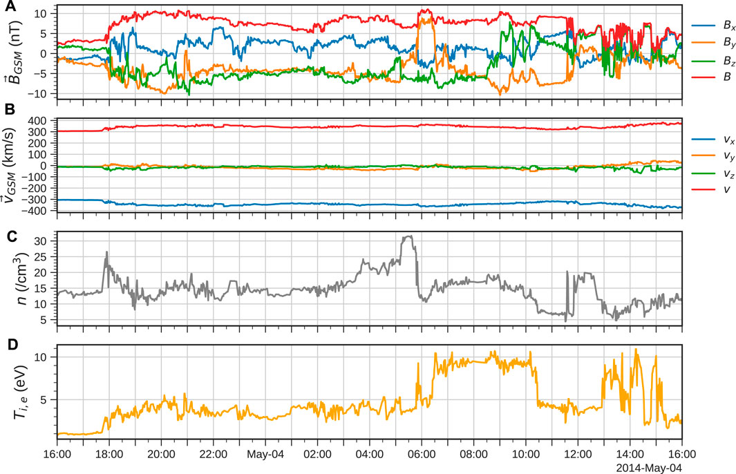
FIGURE 1. Solar wind conditions used to drive the simulation, taken from OMNI. Shown in GSM coordinates are (A) the IMF B, (B) the solar wind velocity v, (C) the number density n and (D) the ion (and electron) temperature Ti,e.
The shock around 05:50 UT on 4 May also coincides with a prominent IMF By reversal, followed by another at 07:00 UT, which should generate strong asymmetries in the tail and so will be of particular interest in our analysis of the current sheet response. In fact, By is negative for almost all of the time for which the IMF is southward, and so there should be a noticeable twisting of the magnetotail throughout. Note the dipole tilt angle ranged from
The Gorgon MHD code models the terrestrial solar wind-magnetosphere interaction by solving the semi-conservative resistive MHD equations on a regular, Eulerian, staggered cartesian grid, and is unique amongst magnetospheric MHD codes in solving for the magnetic vector potential (Ciardi et al., 2007; Mejnertsen et al., 2018; Eggington et al., 2020; Desai et al., 2021a). In this study we utilise a grid with uniform resolution of 0.5 RE, which ensures that the tail is well-resolved at all downtail distances, and a domain spanning X = (−24, 126) RE, Y = (−60, 60) RE, Z = (−60, 60) RE. The time-dependent solar wind parameters are applied at the sunward boundary, with the Earth’s dipole (of moment 7.73 × 10²² Am2) at the origin within the inner boundary of radius 3 RE. Here the FACs are mapped along dipole field lines to a thin-shell ionosphere model where the resulting electrostatic potential is calculated and mapped back out to the magnetosphere to set the plasma flow as an inner boundary condition (Eggington et al., 2018). The ionospheric conductance is calculated from a combination of solar EUV ionization using the empirical formulae of Moen and Brekke, (1993) assuming F10.7 = 100 × 10–22 Wm−2Hz−1, and uniform background polar cap Pedersen and Hall conductances of ΣP = 7 mho and ΣH = 12 mho, respectively, as per Coxon et al. (2016).
To capture the geometric effects of the dipole tilt we use a fixed tilt angle of μ = 15° (the contribution due to the seasonal obliquity of the dipole) and impose the diurnal rotation of the dipole onto the solar wind. The coordinate system is thus related to GSM through a rotation by an angle between ∼±10° in the X-Z plane, depending on the time of day, except that X and Y are defined in the opposite sense. Hence when we transform into GSM for our analysis, the diurnal variation is imposed back onto the dipole which rotates accordingly. The benefit of using a fixed non-zero tilt angle versus the use of Solar Magnetic (SM) coordinates, in which the dipole is fixed along Z (Hapgood, 1992), is greatly reduced solar wind inflow angles hence allowing for a smaller simulation domain. The solar wind data are taken from OMNI and transformed into simulation coordinates by calculating the mean value of μ during the day in question. We inject solar wind for a total of 24 h starting from 16:00 UT on 3 May, with initialisation performed using the relatively quiet 2 h of conditions prior to this window. Since a varying Bx cannot be injected into the simulation box, we simply set the IMF Bx to zero throughout.
One important point to consider is the dependence of the key timescales in the model (e.g., that of global convection) on the model numerics. In the present study we assume ideal MHD by setting the resistivity in the model to zero, such that the Dungey cycle proceeds due to numerical diffusion as is commonly the case with magnetospheric MHD codes. The resulting dynamics will differ between models due to their use of different solvers, grid resolutions/geometries and model parameters such as ionospheric conductance. For example, models can show disagreement in predictions of magnetospheric topology and ionospheric cross-polar cap potential even when driven with the same solar wind conditions (Honkonen et al., 2013; Gordeev et al., 2015). However whilst key timescales in the simulation may be slightly faster or slower than in reality, the simulation still provides valuable insight into the global phenomena driving the system response and complements observations.
To establish the key periods of driving during this event we first investigate the variation in dayside coupling and open flux content in the magnetosphere. The dayside reconnection rate ΦD can be estimated using the solar wind coupling function of Milan et al. (2012), which has the form:
for which Byz is the IMF magnitude in the GSM Y-Z plane and θIMF = arctan (By/Bz) is the IMF clock angle. Whilst the strength of coupling in the simulation may differ slightly from this empirical formula, the general trends should be similar. We can establish this based on the growth and decay in the open flux FPC, which we calculate by integrating the magnetic flux through cells at the outer boundary of the simulation domain which contain open field (Eggington et al., 2022). The magnetic connectivity is determined by tracing field lines from each grid cell and finding where they terminate; open field is defined where one end terminates at the Earth (the North pole for our calculation) and the other in the solar wind (see similarly Honkonen et al., 2011; Aikio et al., 2013; Mejnertsen et al., 2021). Figure 2 shows the variation of these quantities during the first 24 h of the storm, with shading indicating periods in the simulation where either the dayside (ΦD) or nightside (ΦN) reconnection rate dominate, determined simply by whether dFPC/dt is positive or negative, respectively. The initial switch from northward to southward IMF at 18:00 UT on 3 May is associated with a sudden increase in ΦD. This remains relatively high for the following 15 h until the switch back to northward IMF at around 09:00 UT, after which ΦD is generally much lower for the remainder of the event. In that sense the first 24 h of the event can be split into two parts: an extended period of strong, predominantly southward IMF driving, and then a subsequent shorter period of weaker, predominantly northward IMF driving.
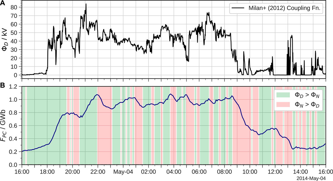
FIGURE 2. Time-series of (A) the estimated dayside reconnection rate ΦD using the coupling function of Milan et al. (2012), and (B) the amount of open magnetic flux FPC in the simulation. Green shading indicates where the dayside rate dominates the nightside rate ΦN, with red indicating the opposite.
The open flux in the simulation gradually increases during the first few hours of the storm, particularly after 18:00 UT on 3 May when the IMF first turns southward. The dayside rate then dominates until around 19:30 UT, with the nightside rate then catching-up and causing a net reduction in FPC over the following hour. Another sudden increase in ΦD around 20:30 UT causes FPC to climb once more to a peak around 22:00 UT. The open flux content then remains close to this elevated level for the remainder of the period of predominantly southward IMF driving, with ΦD and ΦN frequently exceeding one-another. Notably, FPC shows very little variation between 01:30–03:00 UT on 4 May and again between 05:30–08:30 UT. This suggests a dynamical state similar to steady magnetospheric convection (SMC), which arises when the dayside and nightside rates are in relative balance such that tail reconnection can proceed in a laminar fashion (DeJong et al., 2009; Walach and Milan, 2015; Milan et al., 2019). Since SMC can persist for several hours (Walach et al., 2017), the magnetotail current sheet may thus be relatively steady during this period and not disturbed by substorm activity.
After the switch to northward IMF at 09:00 UT the nightside rate dominates as expected (since ΦD becomes very small), closing the majority of the remaining open flux gradually over about 2 h as ΦN decays. This is slightly longer than the duration for which ΦD > ΦN after 18:00 UT, indicating a characteristic global convection timescale of around 1–2 h in the simulation. This is broadly consistent with observations of polar cap contractions: a survey of 25 nightside reconnection events found durations up to 150 min with an average of 70 min (Milan et al., 2007). Note that the same study found values of FPC ranging between 0.2 and 0.9 GWb across all events, comparable to those found here which provides further confidence in the simulation. After around 11:00 UT the dayside rate dominates briefly, but the open flux content then remains low for the remainder of the simulation. This confirms that the latter period of the event should be suitable for studying any distinct modes of response that occur under weaker driving unlike that of the preceding stormtime conditions.
For our analysis of the magnetotail the simulation data are transformed from Gorgon coordinates into an aberrated GSM (AGSM) frame, which has its X-axis anti-parallel with the average GSM solar wind flow direction. This reduces aberration in the tail due to the vy and vz components of the solar wind velocity vector, hence reducing the displacement of the current sheet along the Y- and Z-axes, and has been used in similar studies to account for the ‘windsock’ effect in the magnetotail (e.g. Fairfield, 1980; Hammond et al., 1994; Xiao et al., 2016). To do this, we calculate the average direction of the flow over the preceding 30 min at all times and rotate the GSM X-axis accordingly; this is a sufficient period of time to capture the displacement at the downtail distances considered in our study. As well as allowing for easier analysis, the use of AGSM facilitates direct comparison to studies such as the above.
To examine the behaviour of the magnetotail in response to changes in the IMF, we take slices in the Y-Z plane at a fixed downtail distance. We choose XAGSM = −30 RE initially since this captures both open and closed field depending on the strength of driving (being tailward of the nightside reconnection line during the peak of the storm), with generally strong lobe field hence an intense current sheet. We take a 10 min sliding mean of the magnetic field in the tail (based on three timesteps each 5 min apart) across the whole simulation, which averages-out smaller disturbances to the current sheet making it easier to identify. Figure 3 shows the resulting Bx in the tail over time, as well as the current sheet indicated by the green line and defined as the Bx = 0 contour. Red regions indicate field directed sunward in the northern lobe, and blue indicates anti-sunward field in the southern lobe. The increasing field strength over time demonstrates the loading of open flux in the magnetotail, until the final two panels at 10:00 UT and 12:00 UT which are 1 and 3 h after the IMF has turned northward, respectively. Whilst the reduced flaring in the tail at 10:00 UT demonstrates that the effects of the IMF switch have begun to manifest, the lobe field still remains relatively strong suggesting a delay of
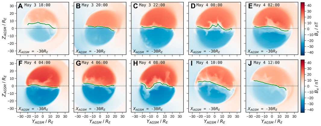
FIGURE 3. Slices (A–J) of the magnetotail at XAGSM = −30 RE showing the lobe field strength Bx over time in 2 h intervals and averaged over a 10 min sliding window. The location of the magnetotail current sheet is shown by the green lines, with the dotted line indicating the AGSM equator.
The variation in the orientation of the current sheet clearly demonstrates the twisting of the magnetotail, which at most times is in a clockwise sense. At 08:00 UT the central portion of the current sheet shows anti-clockwise rotation due to the reversal from negative to positive IMF By just prior to 06:00 UT (at which time the current sheet does not yet appear to be affected), despite the IMF By switching back to negative after 07:00 UT. This suggests a significant delay of
The current sheet is notably less twisted for periods when the tail Bx is strongest under southward IMF, suggesting a stronger twisting under northward IMF (visible from 10:00 UT onwards). During the earlier and later timestamps, there is a clear offset and hinging of the current sheet towards positive ZAGSM (above the dotted line), as expected due to the positive dipole tilt angle which is maximal at around 17:00 UT. The hinging is less apparent when the lobe Bx is strongest around 04:00–06:00 UT, though it is difficult to discern whether this is due to enhanced lobe pressure (and tail reconnection) or due to the tilt angle being near its minimum at this time (see Figure 4C).
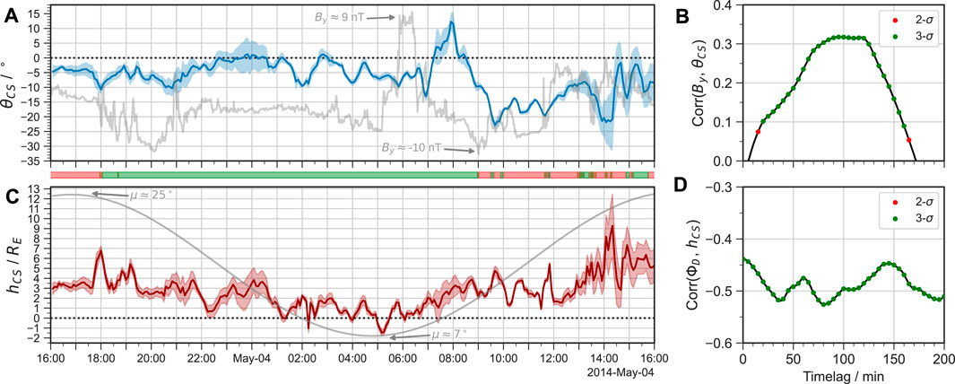
FIGURE 4. Results of the current sheet fitting at XAGSM = −30 RE, showing (A) the rotation angle θCS (blue line) and (C) the hinging parameter hCS (red line) over time, with the shading indicating the uncertainty in the parabolic fit. The variation in (A) the IMF By and (C) the dipole tilt angle μ is indicated by the grey curves to aid with analysis, with extreme values indicated. The colour blocks beneath the time axis of panel (A) indicate intervals when the IMF Bz is positive (red) or negative (green). The correlation coefficient is shown (B,D) for each timelag of the IMF variables, with statistically significant results indicated in red and green for 2-σ and 3-σ significance, respectively.
To investigate the twisting of the current sheet in more detail, we first identify its location in 5 min intervals at XAGSM = −30 RE over the duration of the event, using the method described above with a 10 min sliding window. The twisting of the current sheet due to changes in By is difficult to quantify given its complex time-dependent shape and extent. Therefore, only the portion in the range of |YAGSM| < 15 RE is sampled, so as to accommodate the changing size of the magnetotail and to avoid smearing differing response timescales between the central (small |YAGSM|) and outer (large |YAGSM|) current sheet. This is also motivated by the fact that the central current sheet divides the regions of strongest lobe field, and represents the region most important for nightside reconnection and the asymmetries which manifest in ionospheric coupling.
As we have established, the morphology of the current sheet can be considered a combination of separate effects: these include the twisting due to the IMF By, the hinging due to the dipole tilt, and disturbances due to time-dependent tail reconnection (e.g. at 00:00 UT in Figure 3D), all of which may influence the current sheet incoherently at different Y-positions. In order to extract the first two effects, we fit a second-order polynomial to the current sheet coordinates (YCS, ZCS) of the form:
for some ‘rotation’ angle θCS and ‘hinging’ parameter hCS. The latter is simply the displacement of the current sheet from the AGSM equator as inferred at YAGSM = 0 (for a given XAGSM), and is distinct from the ‘hinging distance’ which is defined in specific current sheet models as the distance between the hinging point and the Earth (e.g., Fairfield, 1980; Hammond et al., 1994; Tsyganenko and Fairfield, 2004; Tsyganenko et al., 2015). The uncertainty in the fitting is found from the root-mean squared (RMS) error, which represents the deviation from an idealised, parabolic current sheet, from which we determine the error in both θCS and hCS. The choice of a simplistic parabolic fit differs from these elliptical models which have performed well at capturing the average current sheet configuration based on large observational datasets (see Xiao et al., 2016 and references therein). However, the time-dependent behaviour of the magnetotail in this case study, combined with the large (and varying) tilt angle, mean a more complex fit is unlikely to provide much benefit and would require more free parameters. Instead, a parabolic fit allows us to effectively deduce the response timescales of the parameters of interest.
The fitting is repeated for each sampled timestep to produce a time-series in the current sheet parameters. We then perform a Pearson cross-correlation of these against time-lagged solar wind parameters to determine the timelag yielding the strongest correlation, representing the characteristic response time. This same approach has been used to deduce equivalent response timescales in the ionospheric FAC and ground magnetic field (Shore et al., 2019; Coxon et al., 2019). We make two assumptions in conducting our cross-correlation analysis: firstly that the rotation depends only on IMF By, and secondly that the hinging depends on the amount of magnetic pressure exerted on the current sheet by the lobes, which increases with the dayside reconnection rate ΦD. For example, Tsyganenko and Fairfield, (2004) found that under southward IMF conditions the current sheet was more rigidly fixed into a tilted configuration than under northward IMF and hence was more deflected in ZGSM. Specifically, this means we cross-correlate θCS with IMF By (in GSM) and hCS with ΦD, the latter as shown in Figure 2A. Periods where the error in each fitted parameter is greater indicate where the current sheet is actively reconfiguring, e.g., during an IMF By reversal. Figure 4 shows these parameters over time, and the results of the cross-correlation.
At the start of the simulation period θCS is weakly negative, such that the current sheet is rotated slightly clockwise, and then shows some variability after the shock arrival at 18:00 UT on 3 May. The IMF By decreases to a minimum around 20:00 UT, before briefly switching to zero around 21:00 UT but then remaining negative. Meanwhile θCS reaches a minimum just before 21:00 UT, but then gradually increases over several hours into an untwisted state (θCS ∼ 0°) in which there is much higher RMS error. This reflects the fact that the current sheet is more disturbed during this period due to reconnection in the tail, as evident in Figure 3D. This weak rotation despite negative IMF By suggests that active nightside reconnection tends to reduce the asymmetry, in agreement with Ohma et al. (2021). For the following several hours until 05:00 UT there is relatively little variability in IMF By, which remains negative. Correspondingly, θCS remains mostly negative but shows more variability than IMF By suggesting time-dependent nightside reconnection is important in determining the extent of the twisting in the tail.
The sharp IMF By reversal around 06:00 UT results in a strong twisting of the current sheet in the opposite direction, with θCS showing a pronounced increase. However this effect is not seen until around 07:00 UT, and θCS only reaches its maximum value of ∼ 12° at 08:00 UT, more than an hour after the IMF By turns negative again. This delay of 1–2 h is indicative of global convection controlling the response. Note that the sharp dynamic pressure decrease which occurs simultaneously to the reversal in IMF By (just prior to 06:00 UT, see Figure 1C) results in an expansion of the magnetosphere which will reduce the pressure in the lobes. However this effect occurs over timescales of minutes, communicated by fast mode waves (e.g., Andreeova et al., 2011; Ozturk et al., 2019), and there is relatively little variation in θCS during the subsequent hour. Therefore whilst the reduced dynamic pressure may affect the extent of the twisting in the tail, which can not easily be separated from direct effects of IMF By, the much larger response after 07:00 UT is specific to the By reversal.
The switch to predominantly northward IMF at ∼ 09:00 UT results in a far stronger twisting in the tail, with θCS reaching a minimum of ∼ − 23° around 09:30 UT. However, this is only 30 min after the IMF By reaches its minimum value at 09:00 UT, suggesting a faster response timescale than under southward IMF conditions. The IMF By then becomes less negative and more variable for the remainder of the simulation, which is also reflected in θCS with the current sheet appearing more disturbed. Another IMF By decrease around 13:30 UT also causes a negative twisting around 14:00 UT, again suggesting a 30 min response under these conditions.
Based on these results there appears to be a bimodal response in the twisting of the current sheet, depending on the strength of driving. However, this is not clearly reflected in the results of the Pearson cross-correlation with the strongest response being over a wide range of timelags from 1–2 h, more consistent with the longer convection timescale under southward IMF. The peak timelag is around 100 min, but this has a fairly weak correlation of ∼ 0.3. However, since the bimodal behaviour throughout the full simulation period may be smearing the overall correlations (which will be highly sensitive to the response to the By reversal), the different periods of driving should be separated to infer the true timescales. This would further reveal if a longer timescale response under northward IMF (as per Browett et al., 2017) is also present, especially further downtail, which we will return to later.
Before proceeding we also briefly discuss the behaviour of the hinging parameter hCS during the simulation. This broadly tracks the variation in the dipole tilt angle, being largest at the start and end of the simulation and reaching a minimum value shortly after the tilt angle is minimal around 05:00 UT. Aside from this there is no particularly clear trend in the response during the most strongly driven period, except for a sharp increase at shock arrival near 18:00 UT on 3 May, with the response being relatively flat during the first few hours of 4 May when FPC is fairly steady (see Figure 2B). Towards the end of the simulation when the driving is weaker the hinging is much more variable and hCS reaches much larger values (albeit with large uncertainty). The correlations with ΦD are consistently negative with 3-σ significance, indicating smaller deflection in Z for southward IMF, which disagrees with the findings of Tsyganenko and Fairfield, (2004). However we note that the 15 h period of strongest dayside coupling also contained most of the 12 h period during which the tilt angle was actively decreasing, which will introduce some bias to the correlations. Regardless, the peak timelag is around 80 min - similar to the 100 min timelag in θCS - and consistent with the delay for open flux to be accumulated in the tail.
To infer whether this behaviour is sensitive to our choice of downtail distance, we repeat the analysis at a series of slices from XAGSM = −15 RE to −70 RE in steps of 5 RE. Note that observations have also shown IMF By signatures within the inner magnetosphere at distances of less than 7 RE (Case et al., 2021), but we limit our analysis only to where the tail field is less dipolar and the current sheet is more twisted. Whilst we also expect twisting further downtail than this range, at such distances the current sheet cannot be as reliably located, in part due to significant aberration of the tail. The result of our current sheet identification is shown for two example timestamps in Figure 5. Note the slices at XAGSM = −15 RE lie just Earthward of the main reconnection line at these times, with the remainder being tailward. The black curve represents the result of the polynomial fitting using equation 3, which performs well where the current sheet has a simple geometry (as at 12:00 UT, bottom row), but results in more error during times of reconfiguration when the current sheet is more disturbed (as at 08:00 UT, top row). This error appears greater further downtail where the Bx = 0 contour is less smooth and the current sheet is significantly more warped. It is clear that the twisting is much stronger further downtail, in agreement with previous studies (Walker et al., 1999; Tsyganenko and Fairfield, 2004). Nonetheless, the sense of the orientation is well-preserved with distance; this suggests a similar twisting timescale in both the near-Earth and middle magnetotail. At 08:00 UT the current sheet is actively reconfiguring in each slice, with the central current sheet rotated oppositely to the outer current sheet. However, our truncation within YAGSM = ± 15 RE is effective at isolating the timescales of the former. Conversely, the current sheet is more uniform at 12:00 UT, being most strongly twisted at XAGSM = −55 RE due to the reduced lobe field strength.
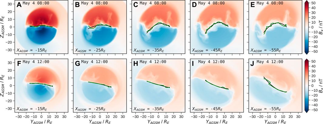
FIGURE 5. Slices of the magnetotail at increasing downtail distances at (A–E) 08:00 UT and (F–J) 12:00 UT on 4 May, showing the lobe field strength Bx over time in 2 h intervals and averaged over a 10 min sliding window. The location of the magnetotail current sheet is shown by the green lines, with the result of the parabolic fitting via Eq. 3 shown by the black curves.
To separate the responses under predominantly southward and northward IMF conditions, we now split our analysis into two distinct periods. To focus on conditions during strong solar wind driving, we select a 15 h window spanning from 18:00 UT on 3 May to 09:00 UT on 4 May. During this time ΦD remains high throughout, resulting in large open flux content and a strong lobe field as evident in Figure 3. For conditions during weaker driving, we select the remaining 7 h time period between 09:00 UT and 16:00 UT for which ΦD was relatively weak; whilst the IMF did occasionally turn southward during this window, this was only brief and there is unlikely to be sufficient flux opening to contaminate the key timescales. With each time-series we then perform a Pearson cross-correlation as before at every downtail distance.
The result for the predominantly southward IMF period is shown in Figure 6. In all cases there is a clear peak timelag that indicates a dominant twisting timescale. Near to the Earth at XAGSM = −15 RE this is relatively short at 40 min, but 20–50 RE downtail the response is strongest around 100 min. From XAGSM = −60 RE to −70 RE this shifts towards slightly shorter timescales, suggesting that the far magnetotail may respond more quickly than the middle and near-Earth magnetotail, presumably due to weaker lobe field. The shorter timelag 15 RE downtail is consistent with the timescales of shear flow-induced By due to MHD wave propagation (Tenfjord et al., 2015), whereas the longer timelag at other distances is consistent with the 1–2 h global convection timescale identified in the simulation. This is reflected in the broader correlation distributions in the near-Earth magnetotail suggesting both timescales are present, whereas the distributions become narrow as the shorter timescale drops off rapidly with distance. Note however that the cross-correlation will be most sensitive to the response to the sharp IMF By reversals, with convection likely proceeding faster (or slower) than 100 min in the near-Earth and middle magnetotail during some periods.
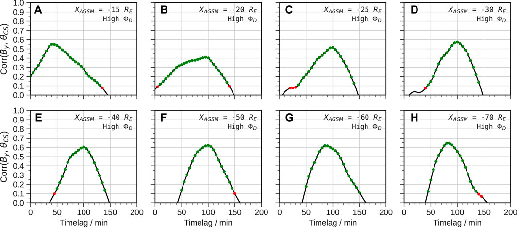
FIGURE 6. Correlations and timelags (A–H) of IMF By versus current sheet rotation angle θCS for multiple downtail distances under high ΦD (predominantly southward IMF) conditions. The scatter points are coloured according to statistical significance as in Figure 4.
For the predominantly northward IMF period the results are markedly different, as shown in Figure 7. Between 15 and 40 RE downtail there is a clear bimodal response: one shorter timescale around 30 min and one much longer response around 2–3 h. The former dominates (with higher correlations) up to 40 RE beyond which it becomes weakly-correlated and is undetectable in the far magnetotail. Here the longer timescale dominates and becomes slower with distance, but with increasing correlations which even exceed that of the equivalent southward IMF timescale. This strongly supports the notion of MHD wave propagation dominating in the near-Earth magnetotail under northward IMF conditions, whereas in the middle and far magnetotail convection-driven reconfiguration controls the twisting and occurs more slowly than under southward IMF.
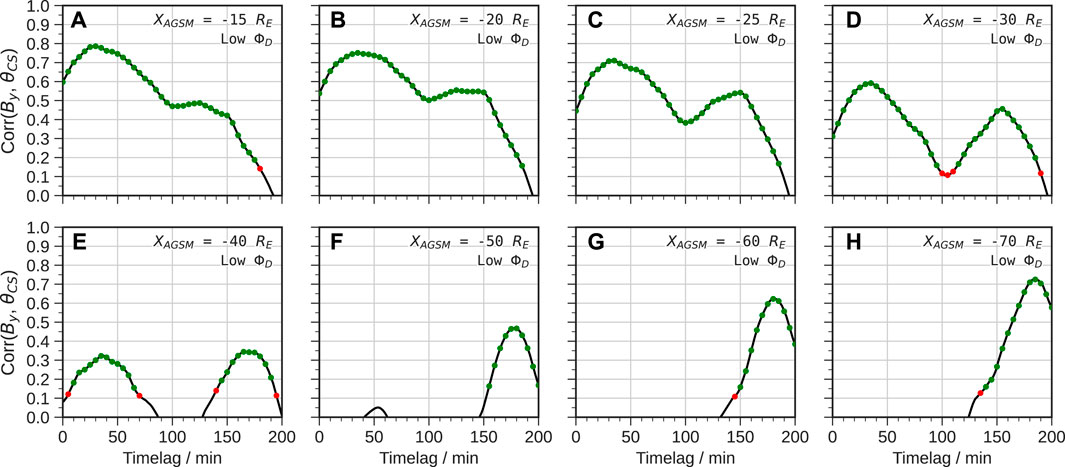
FIGURE 7. Correlations and timelags (A–H) of IMF By versus current sheet angle θCS for multiple downtail distances under low ΦD (predominantly northward IMF) conditions. The scatter points are coloured according to statistical significance as in Figure 4.
The trends described above are summarised for the full range of downtail distances in Figure 8. The mean, minimum and maximum values of θCS are determined across the entire simulation, as well as the peak correlations and timelags under predominantly southward and northward IMF conditions. We also separate out the timelags for the low ΦD period to isolate both the shorter and longer timescale response. In the interest of demonstrating the key trends, we do not discard the strongest timelag even if has less than 2-σ significance. The extent of the rotation clearly grows linearly with distance, although the minimum θCS saturates around XAGSM = −60 RE, which may be a limitation of the parabolic fitting. This trend differs from expectations of magnetotail twisting in induced magnetospheres (for which the draping of field lines should result in a current sheet normal to the IMF, e.g., DiBraccio et al., 2018), demonstrating that the dipole strongly affects the tail configuration even far from the Earth. At all distances the maximum value of θCS corresponds to the sharp IMF By reversal around 06:00 UT on 4 May; near to the Earth this is not sufficient to rotate the current sheet into a strongly positive θCS orientation, but at XAGSM = −70 RE this is as large as ∼ 40°. The largest twisting angles of ∼ -55° at 60–70 RE downtail are comparable with values of up to 50–60° reported by Owen et al. (1995).
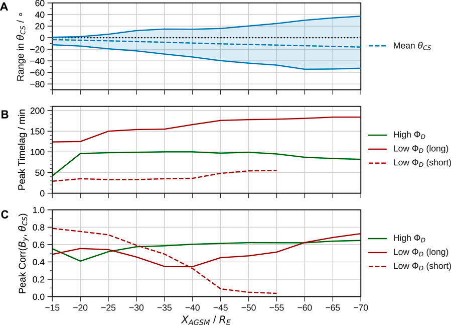
FIGURE 8. Summary of results from the fitting and cross-correlation of θCS. Shown is (A) the range of values over the full simulation, (B) the peak timelags and (C) the peak correlation coefficients for both high and low ΦD separated by mode of response. Note the short timescale for low ΦD is not plotted beyond 55 RE downtail since it is not detectable here.
The peak timelag for high ΦD between 20 and 50 RE downtail is almost identical at ∼ 100 min, and as noted above appears to decrease beyond this (though is still well-correlated at 100 min). In contrast the timescales under northward IMF increase far downtail; this demonstrates that the magnetotail behaves very differently when there is large open flux content versus when it is relatively closed. The trend in the peak correlations also demonstrates that near to the Earth the current sheet is more responsive to IMF By under northward IMF than southward IMF. The high ΦD response is strongest within the mid-tail, with low ΦD correlations again higher in the far-tail over longer timescales, likely since the twisting is more prominent under these conditions. This indicates that global convection is much more effective at controlling the configuration of the middle-to-far magnetotail, and near to the Earth becomes dominated by shorter timescale effects when the system is not being strongly driven. Note the longer convection timescales found here are similar to the ∼ 2–3 h timescale found in observations of tail twisting at distances
In this study we have investigated the response of the magnetotail current sheet to strong, highly variable driving by the solar wind during a geomagnetic storm. The event in question hosted several key features in the IMF, including a switch in Bz from northward to southward and vice-versa, sharp reversals in By, and a prolonged ∼ 15 h period of predominantly southward IMF. This provides a particularly interesting case study for exploring the response timescales of the system, both in terms of the opening and closing of flux in the magnetosphere and the configuration of the magnetotail current sheet. By investigating the change in open flux content we find that the nightside reconnection response to dayside driving is delayed by 1–2 h when the IMF Bz switches sign, due to the gradual accumulation (or lack thereof) of open flux in the magnetotail by global convection.
The variation in flux content is reflected in the lobe magnetic field 30 RE downtail, with the event clearly separated into a period of intense lobe Bx which is sustained for several hours, and then a period of weaker lobe field once open flux is closed under northward IMF. Here the orientation of the current sheet matches the polarity of the IMF By, and clearly twists in response to an IMF By reversal which is more prompt in the outer current sheet than the central portion (|YAGSM| < 15 RE), in agreement with previous simulations with idealised driving (Walker et al., 1999). The extent of the twisting is clearly greater under northward IMF when the lobe magnetic pressure is weakest, such that during the period of most active nightside reconnection the rotation is least noticeable, consistent with observations (Owen et al., 1995; Tsyganenko and Fairfield, 2004; Xiao et al., 2016; Case et al., 2018) and simulations (Ohma et al., 2021).
By focussing on the central current sheet and fitting a parabolic profile at each timestep we have calculated a rotation/twisting angle θCS and hinging parameter hCS of the current sheet over time. We repeated this fitting for a range of downtail distances between 15 and 70 RE, revealing that θCS increases linearly with downtail distance, both in a time-averaged sense and for a more sudden response to an IMF By reversal, consistent with theoretical expectations and empirical models (e.g., Cowley, 1981; Tsyganenko and Fairfield, 2004), and reaching peak angles of rotation similar to those seen in observations (Owen et al., 1995). Focussing our analysis at 30 RE downtail, we find that the hinging generally follows the diurnal trend of the dipole tilt angle during the full 24 h period. Cross-correlation between hCS and an empirical solar wind coupling function also indicates that strong driving acts to reduce the hinging due to enhanced lobe Bx, with a peak timelag of ∼ 80 min across the entire event due to the accumulation of flux in the tail. Meanwhile, θCS responds strongly to a sharp reversal in IMF By when Bz is southward, such that the tail fully untwists into the opposite direction over a period of 1–2 h, also consistent with the timescales of global convection and the response timescale of nightside ionospheric FACs to IMF By identified by Milan et al. (2018) and Coxon et al. (2019). A cross-correlation between θCS and IMF By across the entire event reveals a peak timelag of ∼ 100 min; however, the peak correlation is low (∼ 0.3) indicating that the relationship is more complex and depends on the strength of driving.
To better understand the different modes of response we separated the cross-correlation into two separate periods: one where ΦD was greatest (predominantly southward IMF), and one where ΦD was much lower (predominantly northward IMF). This was repeated for our full range of downtail distances. We find that 20–50 RE downtail the θCS global convection timescale of ∼ 100 min does indeed dominate when ΦD is highest, and is more strongly correlated with IMF By (
The characteristic timescales of the current sheet twisting are summarised in Table 1. Note that since we are fitting simultaneously to a wide portion of the current sheet, our best-correlated ‘response’ will be slower than the initial response of the localised tail By which then reconfigures gradually (see Tenfjord et al., 2017). These timescales will also not always be fixed at the peak timelags identified; for example, convection likely proceeds fastest during the peak of the storm. Overall, our results show that whilst shear flow-induced By is important in controlling asymmetries in the near-Earth magnetotail, the current sheet response appears to be dominated by global convection effects during stronger driving conditions and in general further downtail, such that its role in nightside ionospheric coupling may be less important. Indeed, longer convection timescales of up to 3–4 h during northward IMF can explain observed delays in the response to IMF By in nightside ionospheric FAC (Milan et al., 2018; Coxon et al., 2019) and the formation of auroral arcs (Fear and Milan, 2012; Milan et al., 2005) which have been linked to magnetotail twisting in previous simulations (Kullen and Janhunen, 2004).
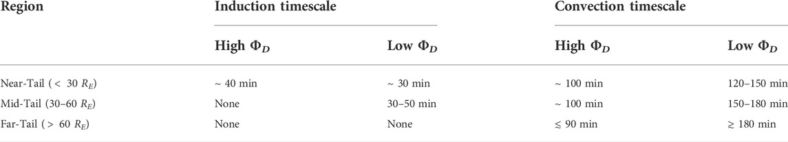
TABLE 1. Summary of different response timescales of the magnetotail current sheet twisting to IMF By during the simulated storm, separated by region of the magnetotail (with downtail distance indicated) and strength of solar wind coupling ΦD. These values are inferred from Figure 8.
Finally, we note some caveats and key points for future work. Whilst our approach isolated the response of the central current sheet for |YAGSM| < 15 RE, the faster outer current sheet response was not captured. An extension of this study could be to deduce the difference in timelag as a function of distance from the X-axis, though this is non-trivial given the complex changes in shape and size of the magnetotail. Our methodology could also be applied to multiple different events to determine how timescales differ for more or less extreme solar wind conditions, and for particular configurations of the magnetosphere with different seasonal tilt angle, such as around equinox. As mentioned in the introduction, various non-MHD effects not captured in the simulation can influence the tail configuration and therefore may be important in determining the timescales of response. For example, smaller-scale flapping motions in the current sheet may affect the extent of the twisting, whilst kinetic effects can control the loading-unloading and thus the large-scale tail dynamics (e.g., Zhang et al., 2020; Kuznetsova et al., 2007). In addition, the inclusion of a ring current in the inner magnetosphere might influence the transport of flux returning to the dayside and thus the length of the Dungey cycle. Future simulation studies incorporating these effects can elucidate whether they play a significant role in determining the global response of the current sheet.
As discussed in Section 2.2, it may be that other global MHD models (such as those used by Walker et al., 1999; Kullen and Janhunen, 2004, Tenfjord et al., 2015) would predict slightly different response timescales than the Gorgon model, for example in shear flow-induced By due to different transit times of MHD waves dependent on the density and field strength (and thus Alfvén speed) in the magnetosphere. However, whilst we do not expect the timescales identified here to match perfectly with reality, the physical interpretations remain the same. A further question is in relating these timescales to those seen in the ionospheric response. A subsequent study will investigate this within our simulation, and compare to observations of the FAC and ground magnetic field timescales to more directly link the magnetospheric and ionospheric asymmetries.
In summary, by simulating the system during highly variable conditions we have identified multiple different modes of magnetotail response. Whilst previous work has disagreed over whether changes in the IMF can be communicated into the system over tens of minutes or over hours, our results instead suggest that both timescales of response can occur, which resolves this apparent disparity in the literature. Changes in the tail morphology due to loading and anti-sunward transport of open flux during southward IMF arise predominantly over convection timescales, and more exaggerated responses under northward IMF occur at both shorter and longer timescales corresponding to wave propagation and the gradual advection of field lines, respectively. Overall, our results have important implications for the understanding of the characteristic timescales over which asymmetries develop in the magnetosphere-ionosphere system and influence space weather.
The raw data supporting the conclusions of this article will be made available by the authors, without undue reservation.
JWBE performed the simulation and analysis presented in the paper, and wrote the manuscript. JCC and RS contributed to the conception of the study and the selection of the simulated event. JCC, RS, RD and JPE provided valuable insight into the work and its direction. LM and JPC are authors of the Gorgon simulation code and its post-processing tools and provided technical guidance for the work.
JWBE was supported by Science and Technology Facilities Council (STFC) Studentship ST/R504816/1. JCC was supported by STFC Ernest Rutherford Fellowship ST/V004883/1. RS was supported by Natural Environment Research Council (NERC) grants NE/V002716/1 and NE/V002732/1. JWBE, LM, JPC and JPE acknowledge funding by NERC grant NE/P017142/1. JWBE, JPC and JPE acknowledge funding by NERC grant NE/V003070/1. RD, JPC and JPE acknowledge funding by NERC grant NE/P017347/1.
This work used the Imperial College High Performance Computing Service (doi: 10.14469/hpc/2232). We acknowledge use of NASA/GSFC’s Space Physics Data Facility’s OMNIWeb service, and OMNI data.
The authors declare that the research was conducted in the absence of any commercial or financial relationships that could be construed as a potential conflict of interest.
All claims expressed in this article are solely those of the authors and do not necessarily represent those of their affiliated organizations, or those of the publisher, the editors and the reviewers. Any product that may be evaluated in this article, or claim that may be made by its manufacturer, is not guaranteed or endorsed by the publisher.
Aikio, A. T., Pitkänen, T., Honkonen, I., Palmroth, M., and Amm, O. (2013). IMF effect on the polar cap contraction and expansion during a period of substorms. Ann. Geophys. 31, 1021–1034. doi:10.5194/angeo-31-1021-2013
Akasofu, S.-I. (2018). A review of the current understanding in the study of geomagnetic storms. Int. J. Earth Sci. Geophys. 4, 1–13. doi:10.35840/2631-5033/1818
Anderson, B. J., Korth, H., Waters, C. L., Green, D. L., Merkin, V. G., Barnes, R. J., et al. (2014). Development of large-scale birkeland currents determined from the active magnetosphere and planetary electrodynamics response experiment. Geophys. Res. Lett. 41, 3017–3025. doi:10.1002/2014GL059941
Andreeova, K., Pulkkinen, T. I., Juusola, L., Palmroth, M., and Santolík, O. (2011). Propagation of a shock-related disturbance in the earth’s magnetosphere. J. Geophys. Res. 116. doi:10.1029/2010JA015908
Borovsky, J. E., Thomsen, M. F., and Elphic, R. C. (1998). The driving of the plasma sheet by the solar wind. J. Geophys. Res. 103, 17617–17639. doi:10.1029/97JA02986
Browett, S. D., Fear, R. C., Grocott, A., and Milan, S. E. (2017). Timescales for the penetration of IMF by into the Earth's magnetotail. J. Geophys. Res. Space Phys. 122, 579–593. doi:10.1002/2016JA023198
Case, N. A., Grocott, A., Haaland, S., Martin, C. J., and Nagai, T. (2018). Response of earth's neutral sheet to reversals in the IMF by component. J. Geophys. Res. Space Phys. 123, 8206–8218. doi:10.1029/2018JA025712
Case, N., Hartley, D., Grocott, A., Miyoshi, Y., Matsuoka, A., Imajo, S., et al. (2021). Inner magnetospheric response to the interplanetary magnetic field by component: Van allen probes and arase observations. JGR. Space Phys. 126. doi:10.1029/2020JA028765
Ciardi, A., Lebedev, S. V., Frank, A., Blackman, E. G., Chittenden, J. P., Jennings, C. J., et al. (2007). The evolution of magnetic tower jets in the laboratory. Phys. Plasmas 14, 056501. doi:10.1063/1.2436479
Cowley, S. W. H., and Lockwood, M. (1992). Excitation and decay of solar wind-driven flows in the magnetosphere-ionosphere system. Ann. Geophys. 10, 103–115.
Cowley, S. W. H. (1981). Magnetospheric asymmetries associated with the y-component of the imf. Planet. Space Sci. 29, 79–96. doi:10.1016/0032-0633(81)90141-0
Coxon, J. C., Milan, S. E., Carter, J. A., Clausen, L. B., Anderson, B. J., and Korth, H. (2016). Seasonal and diurnal variations in AMPERE observations of the Birkeland currents compared to modeled results. J. Geophys. Res. Space Phys. 121, 4027–4040. doi:10.1002/2015JA022050
Coxon, J. C., Rae, I. J., Forsyth, C., Jackman, C. M., Fear, R. C., and Anderson, B. J. (2017). Birkeland currents during substorms: Statistical evidence for intensification of regions 1 and 2 currents after onset and a localized signature of auroral dimming. J. Geophys. Res. Space Phys. 122, 6455–6468. doi:10.1002/2017JA023967
Coxon, J. C., Shore, R. M., Freeman, M. P., Fear, R. C., Browett, S. D., Smith, A. W., et al. (2019). Timescales of birkeland currents driven by the IMF. Geophys. Res. Lett. 2018, 7893–7901. doi:10.1029/2018GL081658
[Dataset] Papitashvili, N. E., and King, J. H. (2020). OMNI 1-min data set [data set]. NASA Space Physics Data Facility.
DeJong, A. D., Ridley, A. J., Cai, X., and Clauer, C. R. (2009). A statistical study of BRIs (SMCs), isolated substorms, and individual sawtooth injections. J. Geophys. Res. 114. doi:10.1029/2008JA013870
Desai, R. T., Eastwood, J. P., Horne, R. B., Allison, H. J., Allanson, O., Watt, C. E. J., et al. (2021a). Drift orbit bifurcations and cross-field transport in the outer radiation belt: Global mhd and integrated test-particle simulations. JGR. Space Phys. 126, e2021JA029802. doi:10.1029/2021JA029802
Desai, R. T., Freeman, M. P., Eastwood, J. P., Eggington, J. W. B., Archer, M. O., Shprits, Y. Y., et al. (2021b). Interplanetary shock-induced magnetopause motion: Comparison between theory and global magnetohydrodynamic simulations. Geophys. Res. Lett. 48, e2021GL092554. doi:10.1029/2021GL092554
DiBraccio, G. A., Luhmann, J. G., Curry, S. M., Espley, J. R., Xu, S., Mitchell, D. L., et al. (2018). The twisted configuration of the martian magnetotail: Maven observations. Geophys. Res. Lett. 45, 4559–4568. doi:10.1029/2018GL077251
Dungey, J. W. (1961). Interplanetary magnetic field and the auroral zones. Phys. Rev. Lett. 6, 47–48. doi:10.1103/PhysRevLett.6.47
Eastwood, J. P., Hapgood, M. A., Biffis, E., Benedetti, D., Bisi, M. M., Green, L., et al. (2018). Quantifying the economic value of space weather forecasting for power grids: An exploratory study. Space weather. 16, 2052–2067. doi:10.1029/2018SW002003
Eggington, J. W. B., Desai, R. T., Mejnertsen, L., Chittenden, J. P., and Eastwood, J. P. (2022). Time-varying magnetopause reconnection during sudden commencement: Global mhd simulations. JGR. Space Phys. 127, e2021JA030006. doi:10.1029/2021JA030006
Eggington, J. W. B., Eastwood, J. P., Mejnertsen, L., Desai, R. T., and Chittenden, J. P. (2020). Dipole tilt effect on magnetopause reconnection and the steady-state magnetosphere-ionosphere system: Global mhd simulations. J. Geophys. Res. Space Phys. 125, e2019JA027510. doi:10.1029/2019JA027510
Eggington, J. W. B., Eastwood, J. P., Mejnertsen, L., Desai, R. T., and Chittenden, J. P. (2018). Forging links in Earth’s plasma environment. Astronomy Geophys. 59, 6. doi:10.1093/astrogeo/aty275
Fairfield, D. (1980). A statistical determination of the shape and position of the geomagnetic neutral sheet. J. Geophys. Res. 85, 775–780. doi:10.1029/JA085iA02p00775
Fear, R. C., and Milan, S. E. (2012). The imf dependence of the local time of transpolar arcs: Implications for formation mechanism. J. Geophys. Res. 117. doi:10.1029/2011JA017209
Gabrielse, C., Angelopoulos, V., Runov, A., and Turner, D. L. (2014). Statistical characteristics of particle injections throughout the equatorial magnetotail. JGR. Space Phys. 119, 2512–2535. doi:10.1002/2013JA019638
Gordeev, E., Sergeev, V., Honkonen, I., Kuznetsova, M., Rastätter, L., Palmroth, M., et al. (2015). Assessing the performance of community-available global mhd models using key system parameters and empirical relationships. Space weather. 13, 868–884. doi:10.1002/2015SW001307
Grocott, A., Milan, S., Yeoman, T., Sato, N., Yukimatu, A., and Wild”, J. (2010). Superposed epoch analysis of the ionospheric convection evolution during substorms: IMF by dependence. J. Geophys. Res. 115. doi:10.1029/2010JA015728
Grocott, A. (2017). Time-dependence of dawn-dusk asymmetries in the terrestrial ionospheric convection pattern” (United States: American geophysical union). Geophys. Monogr., 107–123. doi:10.1002/9781119216346.ch9
Hammond, C. M., Kivelson, M. G., and Walker, R. J. (1994). Imaging the effect of dipole tilt on magnetotail boundaries. J. Geophys. Res. 99, 6079–6092. doi:10.1029/93JA01924
Hapgood, M. A. (1992). Space physics coordinate transformations: A user guide. Planet. Space Sci. 40, 711–717. doi:10.1016/0032-0633(92)90012-D
Honkonen, I., Palmroth, M., Pulkkinen, T. I., Janhunen, P., and Aikio, A. (2011). On large plasmoid formation in a global magnetohydrodynamic simulation. Ann. Geophys. 29, 167–179. doi:10.5194/angeo-29-167-2011
Honkonen, I., Rastätter, L., Grocott, A., Pulkkinen, A., Palmroth, M., Raeder, J., et al. (2013). On the performance of global magnetohydrodynamic models in the earth’s magnetosphere. Space weather. 11, 313–326. doi:10.1002/swe.20055
Kaymaz, Z., Siscoe, G. L., Luhmann, J. G., Lepping, R. P., and Russell, C. T. (1994). Interplanetary magnetic field control of magnetotail magnetic field geometry: Imp 8 observations. J. Geophys. Res. 99, 11113–11126. doi:10.1029/94JA00300
Kullen, A., and Janhunen, P. (2004). Relation of polar auroral arcs to magnetotail twisting and imf rotation: A systematic mhd simulation study. Ann. Geophys. 22, 951–970. doi:10.5194/angeo-22-951-2004
Kuznetsova, M. M., Hesse, M., Rastätter, L., Taktakishvili, A., Toth, G., De Zeeuw, D. L., et al. (2007). Multiscale modeling of magnetospheric reconnection. J. Geophys. Res. 112. doi:10.1029/2007JA012316
Mejnertsen, L., Eastwood, J. P., and Chittenden, J. P. (2021). Control of magnetopause flux rope topology by non-local reconnection. Front. Astron. Space Sci. 8. doi:10.3389/fspas.2021.758312
Mejnertsen, L., Eastwood, J. P., Hietala, H., Schwartz, S. J., and Chittenden, J. P. (2018). Global MHD simulations of the earth’s bow shock shape and motion under variable solar wind conditions. JGR. Space Phys. 123, 259–271. doi:10.1002/2017JA024690
Milan, S. E., Carter, J. A., Sangha, H., Bower, G. E., and Anderson, B. J. (2021). Magnetospheric flux throughput in the dungey cycle: Identification of convection state during 2010. J. Geophys. Res. Space Phys. 126, e2020JA028437. doi:10.1029/2020JA028437
Milan, S. E., Carter, J. A., Sangha, H., Laundal, K. M., Østgaard, N., Tenfjord, P., et al. (2018). Timescales of dayside and nightside field-aligned current response to changes in solar wind-magnetosphere coupling. J. Geophys. Res. Space Phys. 123, 7307–7319. doi:10.1029/2018JA025645
Milan, S. E., Gosling, J. S., and Hubert, B. (2012). Relationship between interplanetary parameters and the magnetopause reconnection rate quantified from observations of the expanding polar cap. J. Geophys. Res. 117. doi:10.1029/2011JA017082
Milan, S. E., Hubert, B., and Grocott, A. (2005). Formation and motion of a transpolar arc in response to dayside and nightside reconnection. J. Geophys. Res. 110, A01212. doi:10.1029/2004JA010835
Milan, S. E., Provan, G., and Hubert, B. (2007). Magnetic flux transport in the dungey cycle: A survey of dayside and nightside reconnection rates. J. Geophys. Res. 112. doi:10.1029/2006JA011642
Milan, S. E., Walach, M.-T., Carter, J. A., Sangha, H., and Anderson, B. J. (2019). Substorm onset latitude and the steadiness of magnetospheric convection. J. Geophys. Res. Space Phys. 124, 1738–1752. doi:10.1029/2018JA025969
Moen, J., and Brekke, A. (1993). The solar flux influence on quiet time conductances in the auroral ionosphere. Geophys. Res. Lett. 20, 971–974. doi:10.1029/92GL02109
Morley, S. K., and Lockwood, M. (2006). A numerical model of the ionospheric signatures of time-varying magnetic reconnection: III. Quasi-Instantaneous convection responses in the cowley-lockwood paradigm. Ann. Geophys. 24, 961–972. doi:10.5194/angeo-24-961-2006
Motoba, T., Hosokawa, K., Ogawa, Y., Sato, N., Kadokura, A., Buchert, S. C., et al. (2011). In situ evidence for interplanetary magnetic field induced tail twisting associated with relative displacement of conjugate auroral features. J. Geophys. Res. 116. doi:10.1029/2010JA016206
Murphy, K. R., Watt, C. E. J., Mann, I. R., Jonathan Rae, I., Sibeck, D. G., Boyd, A. J., et al. (2018). The global statistical response of the outer radiation belt during geomagnetic storms. Geophys. Res. Lett. 45, 3783–3792. doi:10.1002/2017GL076674
Ohma, A., Østgaard, N., Laundal, K. M., Reistad, J. P., Hatch, S. M., and Tenfjord, P. (2021). Evolution of IMF By induced asymmetries: The role of tail reconnection. J. Geophys. Res. Space Phys. 126, e2021JA029577. doi:10.1029/2021JA029577
Oliveira, D. M. (2017). Magnetohydrodynamic shocks in the interplanetary space: A theoretical review. Braz. J. Phys. 47, 81–95. doi:10.1007/s13538-016-0472-x
Owen, C. J., Slavin, J. A., Richardson, I. G., Murphy, N., and Hynds, R. J. (1995). Average motion, structure and orientation of the distant magnetotail determined from remote sensing of the edge of the plasma sheet boundary layer withE> 35 keV ions 35 kev ions. J. Geophys. Res. 100, 185–204. doi:10.1029/94JA02417
Ozturk, D. S., Zou, S., Slavin, J. A., and Ridley, A. J. (2019). Response of the geospace system to the solar wind dynamic pressure decrease on 11 june 2017: Numerical models and observations. J. Geophys. Res. Space Phys. 124, 2613–2627. doi:10.1029/2018JA026315
Petrukovich, A. A. (2011). Origins of plasma sheet by. J. Geophys. Res. 116. doi:10.1029/2010JA016386
Pitkänen, T., Hamrin, M., Kullen, A., Maggiolo, R., Karlsson, T., Nilsson, H., et al. (2016). Response of magnetotail twisting to variations in IMF by : A themis case study 1-2 january 2009. Geophys. Res. Lett. 43, 7822–7830. doi:10.1002/2016GL070068
Rong, Z. J., Lui, A. T. Y., Wan, W. X., Yang, Y. Y., Shen, C., Petrukovich, A. A., et al. (2015). Time delay of interplanetary magnetic field penetration into earth’s magnetotail. J. Geophys. Res. Space Phys. 120, 3406–3414. doi:10.1002/2014JA020452
Rong, Z., Shen, C., Petrukovich, A., Wan, W., and Liu, Z. (2010). The analytic properties of the flapping current sheets in the earth magnetotail. Planet. Space Sci. 58, 1215–1229. doi:10.1016/j.pss.2010.04.016
Sandhu, J. K., Rae, I. J., Freeman, M. P., Forsyth, C., Gkioulidou, M., Reeves, G. D., et al. (2018). Energization of the ring current by substorms. JGR. Space Phys. 123, 8131–8148. doi:10.1029/2018JA025766
Sergeev, V. A. (1987). Penetration of the by component of the IMF into the magnetotail. Geomagnetism Aeronomy 27, 612–615.
Sergeev, V., Runov, A., Baumjohann, W., Nakamura, R., Zhang, T. L., Volwerk, M., et al. (2003). Current sheet flapping motion and structure observed by cluster. Geophys. Res. Lett. 30, 1327. doi:10.1029/2002GL016500
Shore, R. M., Freeman, M. P., Coxon, J. C., Thomas, E. G., Gjerloev, J. W., and Olsen, N. (2019). Spatial variation in the responses of the surface external and induced magnetic field to the solar wind. JGR. Space Phys. 124, 6195–6211. doi:10.1029/2019JA026543
Siscoe, G. L., and Huang, T. S. (1985). Polar cap inflation and deflation. J. Geophys. Res. 90, 543–547. doi:10.1029/JA090iA01p00543
Snekvik, K., Østgaard, N., Tenfjord, P., Reistad, J. P., Laundal, K. M., Milan, S. E., et al. (2017). Dayside and nightside magnetic field responses at 780 km altitude to dayside reconnection. J. Geophys. Res. Space Phys. 122, 1670–1689. doi:10.1002/2016JA023177
Tenfjord, P., Østgaard, N., Haaland, S., Snekvik, K., Laundal, K. M., Reistad, J. P., et al. (2018). How the IMF by induces a local by component during northward IMFBzand characteristic timescales. J. Geophys. Res. Space Phys. 123, 3333–3348. doi:10.1002/2018JA025186
Tenfjord, P., Østgaard, N., Snekvik, K., Laundal, K. M., Reistad, J. P., Haaland, S., et al. (2015). How the IMF by induces a by component in the closed magnetosphere and how it leads to asymmetric currents and convection patterns in the two hemispheres. J. Geophys. Res. Space Phys. 120, 9368–9384. doi:10.1002/2015JA021579
Tenfjord, P., Østgaard, N., Strangeway, R., Haaland, S., Snekvik, K., Laundal, K. M., et al. (2017). Magnetospheric response and reconfiguration times following IMF by reversals. J. Geophys. Res. Space Phys. 122, 417–431. doi:10.1002/2016JA023018
Tsyganenko, N. A., Andreeva, V. A., and Gordeev, E. I. (2015). Internally and externally induced deformations of the magnetospheric equatorial current as inferred from spacecraft data. Ann. Geophys. 33, 1–11. doi:10.5194/angeo-33-1-2015
Tsyganenko, N. A., and Fairfield, D. H. (2004). Global shape of the magnetotail current sheet as derived from geotail and polar data. J. Geophys. Res. 109, A03218. doi:10.1029/2003JA010062
Walach, M.-T., and Milan, S. E. (2015). Are steady magnetospheric convection events prolonged substorms? J. Geophys. Res. Space Phys. 120, 1751–1758. doi:10.1002/2014JA020631
Walach, M.-T., Milan, S. E., Murphy, K. R., Carter, J. A., Hubert, B. A., and Grocott, A. (2017). Comparative study of large-scale auroral signatures of substorms, steady magnetospheric convection events, and sawtooth events. J. Geophys. Res. Space Phys. 122, 6357–6373. doi:10.1002/2017JA023991
Walker, R., Richard, R., Ogino, T., and Ashour-Abdalla, M. (1999). The response of the magnetotail to changes in the imf orientation: The magnetotail’s long memory. Phys. Chem. Earth, Part C Sol. Terr. Planet. Sci. 24, 221–227. doi:10.1016/S1464-1917(98)00032-4
Xiao, S., Zhang, T., Ge, Y., Wang, G., Baumjohann, W., and Nakamura, R. (2016). A statistical study on the shape and position of the magnetotail neutral sheet. Ann. Geophys. 34, 303–311. doi:10.5194/angeo-34-303-2016
Zhang, T. L., Baumjohann, W., Nakamura, R., Balogh, A., and Glassmeier, K.-H. (2002). A wavy twisted neutral sheet observed by cluster. Geophys. Res. Lett. 29, 5. doi:10.1029/2002GL015544
Keywords: magnetotail twisting, current sheet, response timescales, geomagnetic storm, magnetosphere-ionophere coupling, global MHD simulations, space weather
Citation: Eggington JWB, Coxon JC, Shore RM, Desai RT, Mejnertsen L, Chittenden JP and Eastwood JP (2022) Response timescales of the magnetotail current sheet during a geomagnetic storm: Global MHD simulations. Front. Astron. Space Sci. 9:966164. doi: 10.3389/fspas.2022.966164
Received: 10 June 2022; Accepted: 10 August 2022;
Published: 06 September 2022.
Edited by:
Karl Laundal, University of Bergen, NorwayCopyright © 2022 Eggington, Coxon, Shore, Desai, Mejnertsen, Chittenden and Eastwood. This is an open-access article distributed under the terms of the Creative Commons Attribution License (CC BY). The use, distribution or reproduction in other forums is permitted, provided the original author(s) and the copyright owner(s) are credited and that the original publication in this journal is cited, in accordance with accepted academic practice. No use, distribution or reproduction is permitted which does not comply with these terms.
*Correspondence: J. W. B. Eggington, ai5lZ2dpbmd0b24xN0BpbXBlcmlhbC5hYy51aw==
Disclaimer: All claims expressed in this article are solely those of the authors and do not necessarily represent those of their affiliated organizations, or those of the publisher, the editors and the reviewers. Any product that may be evaluated in this article or claim that may be made by its manufacturer is not guaranteed or endorsed by the publisher.
Research integrity at Frontiers
Learn more about the work of our research integrity team to safeguard the quality of each article we publish.