 Fatemeh Bagheri
 Ramon E. Lopez
95% of researchers rate our articles as excellent or good
Learn more about the work of our research integrity team to safeguard the quality of each article we publish.
Find out more
ORIGINAL RESEARCH article
Front. Astron. Space Sci. , 30 September 2022
Sec. Space Physics
Volume 9 - 2022 | https://doi.org/10.3389/fspas.2022.960535
This article is part of the Research Topic Magnetosphere and Ionosphere response to the solar wind transients View all 6 articles
During the main phase of many magnetic storms the solar wind Mach number is low and IMF magnitude is large. Under these conditions, the ionospheric potential saturates, and it becomes relatively insensitive to further increases in the IMF magnitude. On the other hand, the dayside merging rate and the potential become sensitive to the solar wind density. This should result in a correlation between the intensity of the auroral electrojets and the solar wind density. In this study we provide a sample of 314 moderate to strong storms and investigate the correlation between Dst index and the energy dissipated in the ionosphere. We show that for lower Mach numbers, this correlation decreases. We also show that the ionospheric indices of the storms with the lower Mach number are less correlated to the geoeffectiveness of the solar wind during these storms.
As discussed by Gonzalez et al. (1994), the main feature in the solar wind that is responsible for creating geomagnetic storms is an extended period of southward directed Interplanetary Magnetic field (IMF). During a geomagnetic storm, the ring current is strongly enhanced and causes a decrease in the strength of Earth’s horizontal magnetic field which is measured by the Dst or the SYM-H index. The maximum of the magnitude of the Dst has been generally used to classify the intensity of the storms. The total energy in the ring current is related to the Dst index by using Dessler-Parker-Skopke relation (Dessler and Parker, 1959; Sckopke, 1966):
where B◦ is the magnetic field at the surface of the Earth, UM is the magnetic energy of the dipole field beyond the Earth’s surface, and Dst* is the corrected Dst by considering the effects of the solar wind pressure and the quiet time ring current
The physical process behind energy transfer to the magnetosphere-ionosphere system during a geomagnetic storm can be significantly different when the solar wind has a low Mach number (less than about 3.5) (Borovsky et al., 2008; Lavraud and Borovsky, 2008). The difference arises since under the condition of low Mach number the transpolar potential saturates (Lavraud and Borovsky, 2008; Lopez et al., 2010; Myllys et al., 2016), so that the potential becomes less dependent on the IMF Bz magnitude. The saturation effect can be understood by considering the steady-state momentum equation,
The balance between the two forces,
However, the ring current injection rate does not saturate when the ionospheric potential saturates (Russell et al., 2001). Lopez et al. (2009) argued that the reconnection region moves closer to Earth for higher values of solar wind IMF so that the volume per unit magnetic flux in the closed field line region is less for larger negative Bz. Thus, the flux tubes coming from a reconnection region can penetrate deeper into the inner magnetosphere. In other words, the injection of particles into the inner magnetosphere produces more energization and the ring current energy content, hence Dst continues to be dependent on the magnitude of the southward IMF. Therefore, one can conclude that under the conditions of low Mach number solar wind, the ring current (and the Dst Index) will continue to respond to the changes of the magnitude of the southward component of the IMF. However, the potential of the polar cap and consequently the auroral electrojet intensity do not continue to respond strongly to IMF variations when the
In this paper, we provide a sample of 314 moderate to strong storms (Dst index
A starting point for the studies concerning energy dissipation and the roles of solar wind parameters during geomagnetic storms is to make a comprehensive sample of storms. Toward this goal, we use the Dst index provided by the World Data Center for Geomagnetism, Kyoto (http://wdc.kugi.kyoto-u.ac.jp/dstdir/). We define the storm onset by the beginning of a sustained and continuous decrease in the Dst index to at least -50 nT. Using a Python script to mark such events, we identified 314 magnetic storms with the Dst index
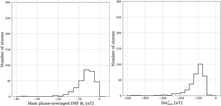
FIGURE 1. Left: Histogram of number of storms in terms of IMF-z component-averaged through main phase. Right: the minimum value of Dst*.
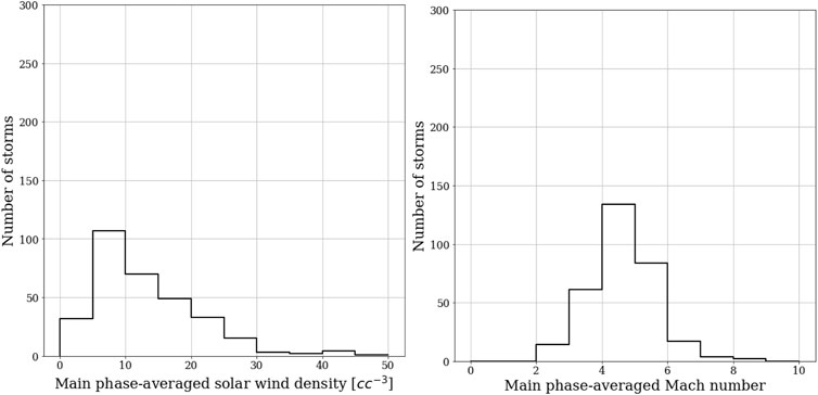
FIGURE 2. Left: Histogram of number of storms in terms of solar wind density-averaged through main phase. Right: Histogram of number of storms in terms of Mach number-averaged through main phase.
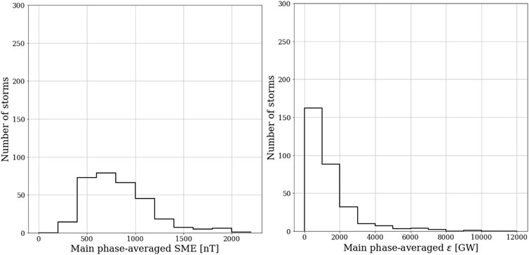
FIGURE 3. Left: Histogram of number of storms in terms of the SME index-averaged through main phase. Right: Histogram of number of storms in terms of the ϵ parameter-averaged through main phase.
As discussed in Introduction, under the condition of low Mach number and high IMF, the ionospheric potential saturates. However, the ring current injection rate does not saturate (Russell et al., 2001). Lopez et al. (2009). Thus under the condition of low Mach number solar wind, the energy in the ring current (as represented the Dst Index) and the energy dissipated in the ionosphere will become uncorrelated since the ionospheric potential and auroral electrojet intensity will not respond strongly to IMF variations while the ring current will. Therefore, the Dst index can be a misleading indicator of the strength of the geomagnetic storm and the amount of energy dissipated in the geospace system under these conditions.
To investigate the relationship between the energy dissipated in the polar ionosphere and the Dst index, we analyze our 314 magnetic storms with Dst∗ ≤ −50 nT for the period between 2000 and 2020. Using the 1-min data from SuperMag for the SME index and the 1-hr solar wind data from OMNI, we estimate the energy dissipated in the ring current, the Joule heating, and the auroral particle precipitation for each storm. For this study, we only estimate the energy involved in the storm’s main phase. To eliminate the influence of the lagtime in the study of the solar wind data and geomagnetic indices, we consider Dst rather than SYM-H as Dst is measured hourly while SYM-H is a 1-min data. This is important since the lagtime between solar wind data and the geomagnetic indices is about 20–35 min (Maggiolo et al., 2017), which has a significant effect when using 1-min data. In addition, O’Brien and McPherron (2000) used Dst rather than SYM-H, and to use those results, we need to use the same index that they used to derive the formula.
As discussed by Burton et al. (1975), the changes in the ring current energy content (hence the changes in the Dst*) is comprised of two terms: the injection term and the proportional loss of the energetic particles,
where τ is the decay time. Empirical studies have been done to determine the decay time (Prigancová and Feldstein, 1992; Valdivia et al., 1996; Mac-Mahon and Gonzalez, 1997; Lu et al., 1998; O’Brien and McPherron, 2000; Xu and Du, 2010). In this paper, we consider τ as described by O’Brien and McPherron (2000),
where V is the solar wind speed, and Bs is the southward IMF component, assuming it is zero if Bz was northward. Thus, we estimate the ring current injection rate, the Joule heating, and the auroral precipitation from equations Eq 5 and Eqs. 2, 3, respectively.
We categorized the storms based on the average value of the magnetosonic Mach number in the main phase of each storm. For each category, we calculated the average of energy dissipated via the ring current injection rate, the Joule heating, and the auroral precipitation over the main phase of storms. Then, we find the Pearson correlation between the Dst* index and the ionospheric power (averaged over the main phase) and between the Dst* index and ring current power. Moreover, since each category a different number of storms (i.e. different sample size), we calculated the standard error for Pearson correlation using the Fisher’s r-to-z transformation method which results in asymmetical confidence intervals. As illustrated in Figure 4-left panel, a lower Mach number leads to a smaller correlation for the ionospheric power. But the ring current injection rate does not show this behavior Figure 5-left panel. In both cases, in the last category related to storms with the Mach number ≥6.5, the standard error in Pearson correlation is relatively high. This is due to the fact that there are only 10 storms in this category therefore the correlation for this sample is not quit reliable compared to the other categories. In Figures 4, 5 right panels show the scatter plot of the main phase-averaged ionospheric power and ring current vs.
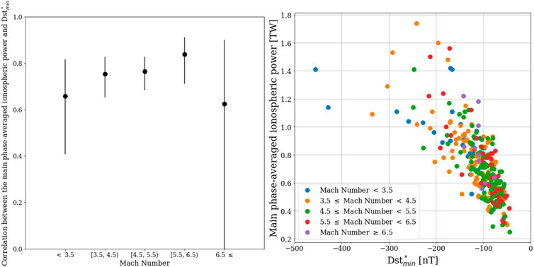
FIGURE 4. right- The Pearson correlation coefficient between the ionospheric power and
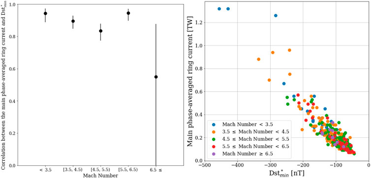
FIGURE 5. left- The Pearson correlation coefficient between the main phased-averaged ring current and
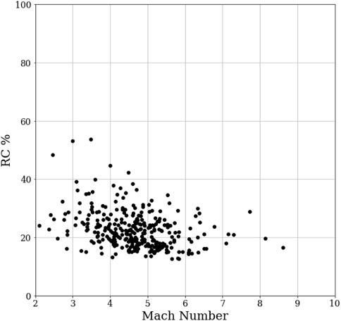
FIGURE 6. The percentage of the energy dissipated in the ring current as a function of averaged Mach number for all 314 storms.
Geoeffectiveness refers to the efficiency of energy coupling from the solar wind into the magnetosphere. As discussed before, during storms with a low Mach number, the ionospheric potential saturates, so that further increases in IMF magnitude results in more magnetosheath flow diversion away from the merging line, decreasing the geoeffective length, and limiting the global merging rate. However, as mentioned earlier, the fact that the ring current injection rate does not saturate suggests that for the low Mach number storm events, geoeffectiveness should be less correlated to the ionospheric potential as compared to events with high Mach number. Again, the fundamental physical mechanism that produces the saturation effect is the shift to a magnetically dominated magnetosheath, where JxB is the largest force diverting the plasma flow. As the solar wind Mach number decreases, the geoeffective length becomes smaller as the JxB force adds to and eventually overtakes the -gradP force diverting the magnetosheath flow away from the dayside merging line. This produces a reduction in geoeffectiveness and a reduced correlation between the IMF and the power dissipated in the geospace system. To show this, in this section, we investigate the relationship between the ionospheric current and the geoeffectivness during magnetic storms.
To define the geoeffectiveness, we should have accurate measurements of the total amount of energy entering the magnetosphere from the solar wind. Although this is not a simple task, different parameters have been defined to estimate the energy input to the magnetosphere. One of them is the ϵ parameter which is defined in (SI units) as
where v is the solar wind speed, B is the magnitude of the IMF, l0 is a characteristic length scale representing the coupling area available for solar wind-magnetosphere interactions, usually approximated as 7RE, (Perreault and Akasofu, 1978), μ0 is the permeability of free space, and θ is defined as
The ϵ parameter is a measure of the rectified Poynting flux in the solar wind times the magnetospheric collecting area. If the IMF was purely southward, the term sin4 (θ/2) reaches its maximum value, and therefore the energy coupling of solar wind and magnetosphere increases significantly. For IMF that is not purely southward, the term (sin4 (θ/2)) reduces the energy input. In this representation, for northward IMF (as long as it is not purely northward) there is still some transfer of energy to the magnetosphere, but at a much reduced rate. The
In addition to ϵ, there are some other parameters to quantify the energy coupling. For instance, one can parameterize solar wind energy input with vBS, where v is the solar wind velocity, and BS is the southward component of the IMF (O’Brien and McPherron, 2000). Another one, defined by Bargatze et al. (1985) which is similar to ϵ in terms of having the sin4 (θ/2), but it is a more complex equation. Similarly, Newell et al. (2007) and Borovsky (2008) have published functions to estimate the magnitude of solar wind-magnetosphere coupling, but these functions share significant similarities with ϵ.
In this section, we discuss the relationship between ϵ, and the SME index during our set of storm events. We use 1-min data of the SME index and 1-min data of ϵ both provided by SuperMag collaborators and can be found at http://supermag.jhuapl.edu/indices/(Gjerloev, 2012). For the first step of studying 314 storms that we have in our sample, we calculate the best linear fit for the SME index as a function of ϵ during the main phase of each storm. Then, similar to the previous section, we categorized the storms based on the average value of the magnetosonic Mach number in the main phase of them. After that, for each category, we calculated the average of the slopes of these linear fits between both data sets. As illustrated in figure Figure 7, as the averaged-Mach number increases, the average of the slopes also increases.
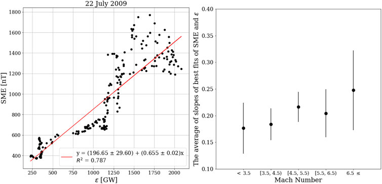
FIGURE 7. left- A sample plot of SME vs. ϵ for the storm happened on 22 July 2009. The linear relationship between the SME index and ϵ can be seen. For more information about this storm look at the table in Supplementary Table S1, row 206. right- The average slopes of the best fits of the SME index as a function of the ϵ for different ranges of averaged Mach number.
Based on the Monte-Carlo simulation, the probability of having a positive trend in Figure 7 is 0.8 (Supplementary Figure S2). Although the trend is visible in Figure 7, but given the values of the slopes, there is not a significant change in the average of slopes for the storms with the Mach number ≤3.5 and with those which has the Mach number between 3.5–4.5. Therefore, the other way to see such a trend is by using the averaged SME index. For each storm, we calculate the average value of the SME index and ϵ during the main phase. Then, similar to the previous sections, for each category of storms (based on the average value of the Mach number), we calculate the Pearson correlation of the averaged-SME index and the averaged-ϵ. Figures 8–10 shows the linear relationship between
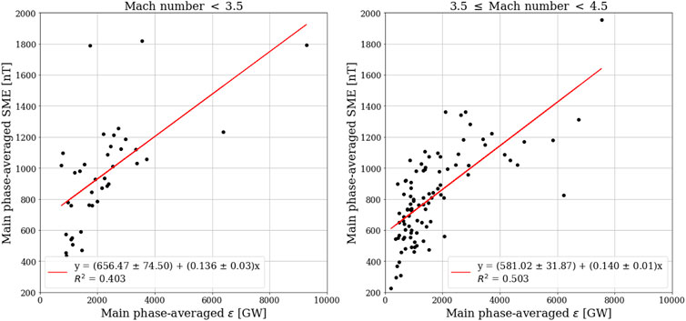
FIGURE 8. The best linear fit of the averaged-SME index and the averaged-ϵ for events with the Mach number: left- ≤ 3.5 right- between 3.5-4.5.
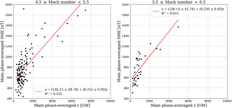
FIGURE 9. The best linear fit of the averaged-SME index and the averaged-ϵ for events with the Mach number: left-between 4.4-5.5 right- between 5.5-6.5.
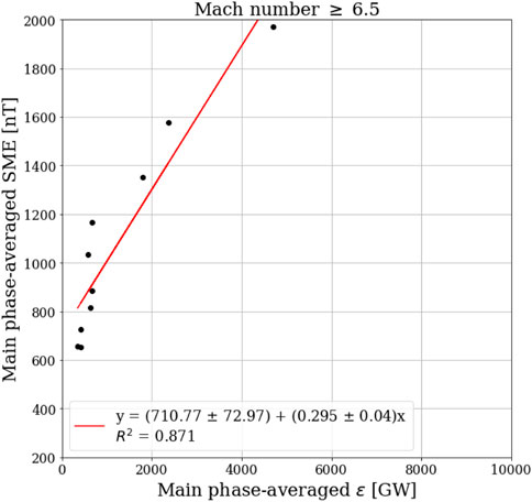
FIGURE 10. he best linear fit of the averaged-SME index and the averaged-ϵ for events with the Mach number
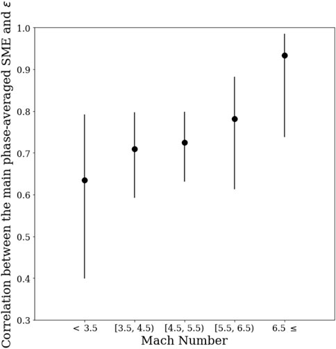
FIGURE 11. The correlation coefficient of the averaged-SME and the averaged-ϵ for different ranges of averaged Mach number.
As discussed in the Introduction, the role of the force balance in the magnetosheath is essential to the understanding of the physics of energy transfer to the magnetosphere-ionosphere system during geomagnetic storms. Lower values of solar wind magnetosonic Mach number are responsible for the reduction of the reconnection line geoeffective length and the saturation of the polar cap potential. The current paradigm for classifying geomagnetic storms is based on the Dst index. However, this paradigm is missing the critical physical process: the ring current injection rate does not saturate while the transpolar potential saturates (Russell et al., 2001; Lopez et al., 2009). We show that for lower Mach numbers, the correlation between the ionospheric power and the Dst index decreases. Therefore, the Dst index is a weak predictor of the ionospheric power for storms with low Mach numbers, which tend to be the large storms when the prediction of ionospheric power dissipation would be particularly important for space weather.
Furthermore, we also show that the ionospheric indices, and hence the power dissipated in the ionosphere, and estimates of the power provided to the magnetosphere by the solar wind are less correlated for the lower Mach number. This result is consistent with the force-balance model since in the saturation regime, by increasing the solar wind energy input, the ionospheric potential remains the same, and the energy dissipates in the ring current and causes the enhancement of the ring current injection rate.
The uncertainty in data can affect the correlation coefficients reported in this paper. Regression bias may exist in this study’s statistics as discussed by sivadasregression. However, the prior assumption in this paper is that the data used in this paper are reliable. Moreover we are averaging over the entire main phase of the storm, and issues like errors in the propagation time of the solar wind data from L1 to Earth should not produce any significant systematic error. Therefore we have confidence in the calculations presented.
One might argue that since these events are magnetic storms in which ionospheric outflow and plasmaspheric plumes are commonly produced, that mass loading of the dayside could reduced the merging rate and account for some or even most of our results. The question of whether local conditions can significantly affect the global integrated merging rate has been the topic of considerable discussion. The two basic positions have been forward by Borovsky and Birn (2014), who argued for local control of the total merging rate, and Lopez (2016), who argued for the dominance of global control based on the force-balance model. However, recent theoretical (Dorelli, 2019) and observational (Zou et al., 2021) evidence strongly favor the global control argument, which is based on the force-balance model and which is consistent with the results represented here.
We gratefully acknowledge the SuperMAG website and the data there provided by SuperMAG collaborators. The SME data can be found at http://supermag.jhuapl.edu/indices/for the periods described in the paper. We thank the AMPERE team and the AMPERE Science Center for providing the Iridium-derived data products. The AMPERE Birkeland current data can be found at http://ampere.jhuapl.edu/products/itot/daily.html for each day at a 2-min time resolution. We acknowledge the use of the OMNI data set, which was obtained from CDAWeb using the Space Physics Data Facility (SPDF) https://cdaweb.gsfc.nasa.gov/pub/data/omni/high_res_omni/monthly_1min/. We acknowledge the support of the US National Science Foundation (NSF) under Grant No. 1916604. We also acknowledge the support of The National Aeronautics and Space Administration (NASA) under Grant No. 80NSSC20K0606 (The Center for the Unified Study of Interhemispheric Asymmetries (CUSIA)) and Grant No. 80NSSC21K2057.
The original contributions presented in the study are included in the article/Supplementary Material further inquiries can be directed to the corresponding author.
FB did this research as a Ph.D. student under the supervision of RL. All authors contributed to manuscript revision, read, and approved the submitted version.
The authors declare that the research was conducted in the absence of any commercial or financial relationships that could be construed as a potential conflict of interest.
All claims expressed in this article are solely those of the authors and do not necessarily represent those of their affiliated organizations, or those of the publisher, the editors and the reviewers. Any product that may be evaluated in this article, or claim that may be made by its manufacturer, is not guaranteed or endorsed by the publisher.
The Supplementary Material for this article can be found online at: https://www.frontiersin.org/articles/10.3389/fspas.2022.960535/full#supplementary-material
Akasofu, S. I. (1981). Energy coupling between the solar wind and the magnetosphere. Space Sci. Rev. 28, 121–190. doi:10.1007/bf00218810
Bargatze, L., McPherron, R., and Baker, D. (1985). “Solar wind-magnetosphere energy input functions,” in Tech. rep. (Los Angeles, USA: California Univ., Dept. of Earth and Space Sciences …).
Baumjohann, W., and Kamide, Y. (1984). Hemispherical joule heating and the ae indices. J. Geophys. Res. 89, 383–388. doi:10.1029/ja089ia01p00383
Borovsky, J. E., and Birn, J. (2014). The solar wind electric field does not control the dayside reconnection rate. J. Geophys. Res. Space Phys. 119, 751–760. doi:10.1002/2013ja019193
Borovsky, J. E., Hesse, M., Birn, J., and Kuznetsova, M. M. (2008). What determines the reconnection rate at the dayside magnetosphere? J. Geophys. Res. 113. doi:10.1029/2007ja012645
Borovsky, J. E. (2021). On the saturation (or not) of geomagnetic indices. Front. Astron. Space Sci. 8, 740811. doi:10.3389/fspas.2021.740811
Borovsky, J. E. (2008). The rudiments of a theory of solar wind/magnetosphere coupling derived from first principles. J. Geophys. Res. 113. doi:10.1029/2007ja012646
Burton, R., McPherron, R., and Russell, C. (1975). An empirical relationship between interplanetary conditions and dst. J. Geophys. Res. 80, 4204–4214. doi:10.1029/ja080i031p04204
Dessler, A., and Parker, E. N. (1959). Hydromagnetic theory of geomagnetic storms. J. Geophys. Res. 64, 2239–2252. doi:10.1029/jz064i012p02239
Dorelli, J. C. (2019). Does the solar wind electric field control the reconnection rate at Earth’s subsolar magnetopause? J. Geophys. Res. Space Phys. 124, 2018JA025868–2681. doi:10.1029/2018ja025868
Gjerloev, J. (2012). The supermag data processing technique. J. Geophys. Res. 117. doi:10.1029/2012ja017683
Gonzalez, W., Joselyn, J. A., Kamide, Y., Kroehl, H. W., Rostoker, G., Tsurutani, B., et al. (1994). What is a geomagnetic storm? J. Geophys. Res. 99, 5771–5792. doi:10.1029/93ja02867
Lavraud, B., and Borovsky, J. E. (2008). Altered solar wind-magnetosphere interaction at low mach numbers: Coronal mass ejections. J. Geophys. Res. 113. doi:10.1029/2008ja013192
Lopez, R., Bruntz, R., Mitchell, E., Wiltberger, M., Lyon, J., and Merkin, V. (2010). Role of magnetosheath force balance in regulating the dayside reconnection potential. J. Geophys. Res. 115. doi:10.1029/2009ja014597
Lopez, R. E. (2016). The integrated dayside merging rate is controlled primarily by the solar wind. JGR. Space Phys. 121, 4435–4445. doi:10.1002/2016ja022556
Lopez, R., Lyon, J., Mitchell, E., Bruntz, R., Merkin, V., Brogl, S., et al. (2009). Why doesn’t the ring current injection rate saturate? J. Geophys. Res. 114. doi:10.1029/2008ja013141
Lopez, R., Wiltberger, M., Hernandez, S., and Lyon, J. (2004). Solar wind density control of energy transfer to the magnetosphere. Geophys. Res. Lett. 31, L08804. doi:10.1029/2003gl018780
Lu, G., Baker, D., McPherron, R., Farrugia, C. J., Lummerzheim, D., Ruohoniemi, J., et al. (1998). Global energy deposition during the january 1997 magnetic cloud event. J. Geophys. Res. 103, 11685–11694. doi:10.1029/98ja00897
Mac-Mahon, R. M., and Gonzalez, W. (1997). Energetics during the main phase of geomagnetic superstorms. J. Geophys. Res. 102, 14199–14207. doi:10.1029/97ja01151
Maggiolo, R., Hamrin, M., De Keyser, J., Pitkänen, T., Cessateur, G., Gunell, H., et al. (2017). The delayed time response of geomagnetic activity to the solar wind. J. Geophys. Res. Space Phys. 122, 11–109. doi:10.1002/2016ja023793
Myllys, M., Kilpua, E., Lavraud, B., and Pulkkinen, T. (2016). Solar wind-magnetosphere coupling efficiency during ejecta and sheath-driven geomagnetic storms. J. Geophys. Res. Space Phys. 121, 4378–4396. doi:10.1002/2016ja022407
Newell, P., Sotirelis, T., Liou, K., Meng, C. I., and Rich, F. (2007). A nearly universal solar wind-magnetosphere coupling function inferred from 10 magnetospheric state variables. J. Geophys. Res. 112. doi:10.1029/2006ja012015
O’Brien, T. P., and McPherron, R. L. (2000). An empirical phase space analysis of ring current dynamics: Solar wind control of injection and decay. J. Geophys. Res. 105, 7707–7719. doi:10.1029/1998ja000437
Østgaard, N., Germany, G., Stadsnes, J., and Vondrak, R. (2002a). Energy analysis of substorms based on remote sensing techniques, solar wind measurements, and geomagnetic indices. J. Geophys. Res. 107, 1233. doi:10.1029/2001ja002002
Østgaard, N., Vondrak, R., Gjerloev, J., and Germany, G. (2002b). A relation between the energy deposition by electron precipitation and geomagnetic indices during substorms. J. Geophys. Res. 107, 1246. doi:10.1029/2001ja002003
Perreault, P., and Akasofu, S. (1978). A study of geomagnetic storms. Geophys. J. Int. 54, 547–573. doi:10.1111/j.1365-246x.1978.tb05494.x
Prigancová, A., and Feldstein, Y. I. (1992). Magnetospheric storm dynamics in terms of energy output rate. Planet. space Sci. 40, 581–588. doi:10.1016/0032-0633(92)90272-p
Russell, C., Luhmann, J., and Lu, G. (2001). Nonlinear response of the polar ionosphere to large values of the interplanetary electric field. J. Geophys. Res. 106, 18495–18504. doi:10.1029/2001ja900053
Sckopke, N. (1966). A general relation between the energy of trapped particles and the disturbance field near the Earth. J. Geophys. Res. 71, 3125–3130. doi:10.1029/jz071i013p03125
Shue, J. H., and Kamide, Y. (2001). Effects of solar wind density on auroral electrojets. Geophys. Res. Lett. 28, 2181–2184. doi:10.1029/2000gl012858
Valdivia, J., Sharma, A., and Papadopoulos, K. (1996). Prediction of magnetic storms by nonlinear models. Geophys. Res. Lett. 23, 2899–2902. doi:10.1029/96gl02828
Vasyliūnas, V. M., and Song, P. (2005). Meaning of ionospheric joule heating. J. Geophys. Res. 110, A02301. doi:10.1029/2004ja010615
Xu, W. Y., and Du, A. M. (2010). Effects of the ring current decay rate on the energy state of the magnetosphere. Chin. J. Geophys. 53, 329–338. doi:10.1002/cjg2.1501
Keywords: dst index, force-balance model, geoeffectiveness, magnetic storms, mach number
Citation: Bagheri F and Lopez RE (2022) Solar wind magnetosonic mach number as a control variable for energy dissipation during magnetic storms. Front. Astron. Space Sci. 9:960535. doi: 10.3389/fspas.2022.960535
Received: 03 June 2022; Accepted: 26 August 2022;
Published: 30 September 2022.
Edited by:
David Gary Sibeck, National Aeronautics and Space Administration, United StatesReviewed by:
Benoit Lavraud, UMR5804 Laboratoire d’astrophysique de Bordeaux (LAB), FranceCopyright © 2022 Bagheri and Lopez. This is an open-access article distributed under the terms of the Creative Commons Attribution License (CC BY). The use, distribution or reproduction in other forums is permitted, provided the original author(s) and the copyright owner(s) are credited and that the original publication in this journal is cited, in accordance with accepted academic practice. No use, distribution or reproduction is permitted which does not comply with these terms.
*Correspondence: Fatemeh Bagheri, ZnhiMTQ5NUBtYXZzLnV0YS5lZHU=
Disclaimer: All claims expressed in this article are solely those of the authors and do not necessarily represent those of their affiliated organizations, or those of the publisher, the editors and the reviewers. Any product that may be evaluated in this article or claim that may be made by its manufacturer is not guaranteed or endorsed by the publisher.
Research integrity at Frontiers
Learn more about the work of our research integrity team to safeguard the quality of each article we publish.