 S. M. Hatch
 K. M. Laundal
  J. P. Reistad
 - Birkeland Centre for Space Science, Department of Physics and Technology, University of Bergen, Bergen, Norway
It is often assumed that on average, polar ionospheric electrodynamics in the Northern and Southern Hemispheres are mirror symmetric or antisymmetric with respect to the interplanetary magnetic field By component and the dipole tilt angle ψ. For example, one might assume that the average Birkeland current density j at magnetic latitude λ is equal to the current density at magnetic latitude −λ if the signs of By and ψ are reversed and all other parameters are equal: j(λ, By, ψ, … ) = j(−λ, −By, −ψ, … ). This is a convenient assumption for empirical models, since it effectively doubles the amount of information that a measurement made in one hemisphere contains. In this study we use the Average Magnetic field and Polar current System (AMPS) model to quantify to what extent the assumption holds for Birkeland and ionospheric currents. The AMPS model is an empirical model based on Swarm and CHAMP magnetic field measurements, with no constraints on hemispheric symmetries, and with differences in main magnetic field geometry as well as biases in data point distributions in magnetic coordinates accounted for. We show that when averaged over IMF clock angle orientation, the total ionospheric divergence-free current in each hemisphere largely satisfies the mirror symmetry assumption. The same is true for the total Birkeland current in each hemisphere except during local winter, during which the Northern Hemisphere tends to dominate. We show that this local winter asymmetry is consistent with the average winter hemispheric asymmetry in total precipitating electron current derived from Fast Auroral SnapshoT (FAST) satellite observations. We attribute this and other more subtle deviations from symmetry to differences in sunlight distribution in magnetic coordinates, as well as magnetic field strength and its influence on ionospheric conductivity. Important departures from mirror symmetry also arise for some IMF clock angle orientations, particularly those for which IMF Bz > 0, as suggested by other recent studies.
1 Introduction
The large-scale polar ionospheric electrodynamics is on average largely mirror symmetric between hemispheres with respect to the interplanetary magnetic field (IMF) By component and the dipole tilt angle. This means that the average magnetic field perturbation (or equivalent current), plasma flow velocity (or equivalent electric field), or electric conductivity found in one hemisphere would be approximately equal to the corresponding quantity in the opposite hemisphere, on the same main magnetic field line, if the signs of the IMF By and the dipole tilt angle had been reversed. This property has been established through numerous climatological studies of plasma flows (e.g., Heppner and Maynard, 1987; Pettigrew et al., 2010; Förster and Haaland, 2015), magnetic fields (e.g., Mead and Fairfield, 1975), and magnetic field perturbations (e.g., Green et al., 2009; Laundal et al., 2016a; Smith et al., 2017). To our knowledge it has not been systematically addressed in climatological studies of auroras or particle precipitation, yet it has been surmised for decades (Gussenhoven et al., 1983; Hardy et al., 1985; Newell et al., 2009, 2010; Dombeck et al., 2018; Zhu et al., 2021). The nearest to directly addressing hemispheric asymmetries in particle precipitation is perhaps Newell and Meng (1988); Hatch et al. (2018) also address hemispheric asymmetries of precipitation associated with Alfvén waves.
The reasons for the symmetry properties of By and tilt are believed to be well understood. The dipole tilt angle describes the orientation of the Earth’s magnetic dipole axis with respect to the Sun-Earth line, and it ranges from about − 30° to + 30°. The variation in tilt angle is thought to have two primary effects: a change in the solar wind-magnetosphere coupling, and a change in ionospheric conductivity due to differences in insolation. The former effect is due to a change in the geometry of the coupling between the solar wind and magnetosphere, and includes a change in the prevalence of lobe reconnection (Crooker and Rich, 1993; Reistad et al., 2019). These variations are presumably almost perfectly mirror symmetrical between hemispheres, since the Earth’s magnetic field in the outer magnetosphere is symmetric between hemispheres. Some have also suggested that the change in geometry influences the subsolar reconnection location and efficiency (e.g., Russell et al., 2003), although this point is contested (Lockwood et al., 2020). The other dipole tilt angle effect—variable ionospheric conductivity due to variations in insolation—alters magnetosphere-ionosphere interactions, with distinct consequences for current patterns (Laundal et al., 2016b,a; Green et al., 2009; Laundal et al., 2018).
The asymmetries associated with the IMF By component are likewise ultimately an effect of different reconnection geometries and configurations on the dayside of the magnetosphere. When By is positive, newly opened magnetic flux experiences a force towards dawn in the Northern Hemisphere, creating dawnward plasma flow on the dayside in the polar ionosphere. In the Southern Hemisphere the force is toward dusk and the plasma flow is duskward. When By is negative, the senses of these forces and flows in the two hemispheres reverse. These effects collectively give rise to a pattern of magnetic perturbations (and corresponding currents via ∇ ×B = μ0 J) known as the Svalgaard-Mansurov effect (Jørgensen et al., 1972). The lateral motion of newly opened flux creates an asymmetric pressure distribution in the magnetotail lobes, which induces a slight asymmetry in the magnetic field mapping to the high latitudes. This asymmetry manifests as an apparent longitudinal shift between hemispheres of conjugate field lines compared to their nominal configuration (Tenfjord et al., 2015). The asymmetry reverses when By changes sign; that is, it exhibits mirror symmetry.
From the standpoint of modeling and statistical studies, the utility of assuming hemispheric mirror symmetry/anti-symmetry is that it effectively doubles the amount of information that a measurement provides. This assumption is therefore useful in dealing with data sets where the number of measurements made in one hemisphere (almost invariably the Southern) are deemed too few for a statistical study, or when measurements made by sun-synchronous satellites (e.g., the Defense Meteorological Satellite Program, or DMSP, satellites), whose orbits cover only a portion of the high-latitude ionosphere in magnetic latitude-magnetic local time (MLat-MLT) coordinates in each hemisphere. In such cases, the only alternative to assuming mirror symmetry is to ignore one hemisphere (Weimer, 2013; Waters et al., 2015; Billett et al., 2018; Thomas and Shepherd, 2018).
Thus the assumption of mirror symmetry has often been what enables a comparison of the two hemispheres to be carried out or an empirical model to be created. Studies and models falling into this category address a broad range of topics, including the ionospheric electric potential (Papitashvili et al., 1994; Weimer, 2005; Zhu et al., 2021), conductance (McGranaghan et al., 2015), field-aligned currents (Weimer, 2001), frictional heating and Poynting flux (Weimer and Edwards, 2021), auroral precipitation (Hardy et al., 1985; Newell et al., 2009, 2010; McGranaghan et al., 2021; Zhu et al., 2021) and even auroral boundaries (Gussenhoven et al., 1983). Other examples include models of the magnetospheric magnetic field, which make use of mirror symmetry with respect to dipole tilt angle (Mead and Fairfield, 1975; Andreeva and Tsyganenko, 2016).
There are a number of reasons to believe that the mirror symmetry suggested by the effects mentioned above is in fact not exact, first among which are that its inexactness is experimentally established. For example, Pettigrew et al. (2010) report that the cross-polar cap potential is on average several percent larger in the Southern Hemisphere. On the basis of the Iridium® satellites and the Swarm satellites, respectively, Green et al. (2009) and Workayehu et al. (2020) report a hemispheric asymmetry in ratios of total currents flowing into each hemisphere for different seasons and reported that Southern Hemisphere currents are overall weaker. A number of studies have shown (Knipp et al., 2021; Pakhotin et al., 2021; Cosgrove et al., 2022) or suggested (Hatch et al., 2018) that deposition of magnetosphere-origin Poynting flux into the ionosphere is greatest in the Northern Hemisphere. Furthermore, although investigations of the magnetic field near the equatorial plane in the magnetosphere show a large degree of mirror symmetry with respect to IMF By and dipole tilt, there are certainly non-symmetric features present as well (e.g., Cowley and Hughes, 1983; Petrukovich, 2011; Tenfjord et al., 2017). (Additionally, away from the equatorial plane very little investigation of IMF By and dipole tilt dependence has been conducted.)
Beyond this direct experimental evidence, many of the parameters that govern magnetosphere-ionosphere-atmosphere interactions exhibit hemispheric asymmetry. These include hemispheric asymmetries (in coordinate systems organized by Earth’s magnetic field) in magnetic field intensity and inclination (Thébault et al., 2015; Laundal et al., 2017), insolation (e.g., Laundal et al., 2017; Hatch et al., 2020), neutral winds (Dhadly et al., 2019), thermospheric composition and temperature (Barlier et al., 1974; Mayr and Trinks, 1977; Qin et al., 2008), and ionospheric densities and temperatures (e.g., Laundal et al., 2019; Hatch et al., 2020; Pignalberi et al., 2021). All of these parameters have some influence on magnetosphere-ionosphere-atmosphere interactions. In terms of quasi-static ionospheric electrodynamics (see, e.g., Richmond, 1995a; Vasyliunas, 2012), their influence is chiefly manifest through the dependence of Pedersen and Hall conductivities in the ionospheric Ohm’s law on them, and through the variation of the frame of reference in which this law is typically expressed, which is that of the height-dependent neutral wind (e.g., Strangeway, 2012).
On point of hemispheric differences in insolation, Figure 1 shows quasi-dipole (QD) coordinate (Richmond, 1995a) grids in geographic coordinates in the two hemispheres, and contour plots of magnetic field strength, using the International Geomagnetic Reference Field (IGRF) model (Thébault et al., 2015). Insolation is symmetric with respect to Earth’s geographic poles; thus the displacement of the geomagnetic poles as well as the distortion of lines of magnetic latitude and longitude with respect to geographic latitudes clearly indicates that insolation of the magnetic high-latitude regions is asymmetric.
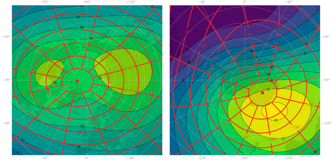
FIGURE 1. Illustration of the differences in Earth’s magnetic field in the north (left) and south (right). The colored contours show the IGRF main field magnitude at epoch=2015.0 with contour levels labeled in μT. The red curves represent magnetic apex coordinate grids. Both plots are stereographic projections of an equally large area, centered at the geographic poles. Geographic longitudes are indicated at the edges.
Last, in addition to these parameters that explicitly appear in the governing equations of ionospheric electrodynamics, the possible influence of non-local (with respect to the ionosphere) and kinetic parameters that exhibit hemispheric asymmetries, including magnetospheric plasma density (Haaland et al., 2017), exospheric neutral composition (Keating et al., 1973), and mesosphere/lower-thermosphere dynamics as well as cloud microphysics (Xie et al., 2021), is unknown. In particular, there are significant hemispheric differences in the tidal behavior of mesospheric and lower thermospheric winds (Avery et al., 1989; Vincent, 2015); to our knowledge, how these differences might affect ionospheric dynamics has not been explored.
In this paper, we use a recent empirical model to quantify how much the ionospheric current system in the two hemispheres diverges from mirror symmetry. This model was designed to account for differences in the structure of the earth’s magnetic field and for differences in spacecraft sampling. In Section 2 we describe the model. In Section 3 we examine how well the mirror symmetry assumption j(λ, By, ψ, … ) = j(−λ, −By, −ψ, … ) holds for ionospheric and Birkeland current densities by examining model current densities and integrated currents in each hemisphere, and present a comparison of our results with those of the Iridium®-based Coxon et al. (2016) study. In Section 4 we discuss these results and some additional sources of uncertainty, including the possible variation of ionospheric currents with magnetic longitude, and conclude.
2 Methodology
The tool that we use to test hemispheric mirror symmetry is the Average Magnetic Field and Current System (AMPS) model. This is an empirical model of the three-dimensional current system, presented by Laundal et al. (2018), based on ionospheric magnetic field measurements from the CHAMP and Swarm satellites. The ionospheric perturbation magnetic field is obtained by subtracting the CHAOS model field (Finlay et al., 2020), which models internal and magnetospheric fields, from spacecraft measurements. The ionospheric magnetic perturbation field is represented as a sum of poloidal and toroidal fields, which are in turn represented as functions of scalar potentials expanded in a series of spherical harmonics. See Laundal et al. (2016a) for a full discussion of this technique.
The AMPS model coefficients depend explicitly on IMF clock angle
and the related quantity
In this paper we use the publicly available Python implementation of the AMPS model, pyAMPS (Laundal and Toresen, 2018), to calculate associated horizontal and field-aligned current densities, projected on a sphere at 110 km altitude. The most recent update includes Swarm magnetic field measurements through 5 February 2021.
The AMPS model is well suited to test hemispheric symmetries because 1) no constraints on hemispheric symmetry were applied in the derivation of the model, and 2) geometric distortions associated with the Earth’s main field were taken into account by use of magnetic apex coordinates (Richmond, 1995b).
3 Results
In this section we present AMPS model current densities from the Northern Hemisphere together with Southern Hemisphere current densities for which the signs of the dipole tilt angle and IMF By component have been reversed.
3.1 Birkeland currents
Figures 2–4 show Birkeland currents for negative, zero, and positive dipole tilt angles (respectively winter, equinox, and summer in the Northern Hemisphere), with a transverse IMF component BT = 4 nT, and solar wind speed vx = −350 km/s. The current densities in the Northern Hemisphere are shown with filled contours, with magnitudes indicated by the color scale at the bottom of the figure. The current densities in the Southern Hemisphere are shown with black contours, solid for positive (upward) values and dashed for negative. The steps between each contour represents a change of 0.05μA/m2, the same as for the colored contours. The eight subplots in each figure represent different IMF orientations, indicated by the clock angle diagram in the center. Again, the sign of By is reversed for the Southern Hemisphere, so that the left column represents negative By for the Northern Hemisphere but positive By for the Southern Hemisphere.
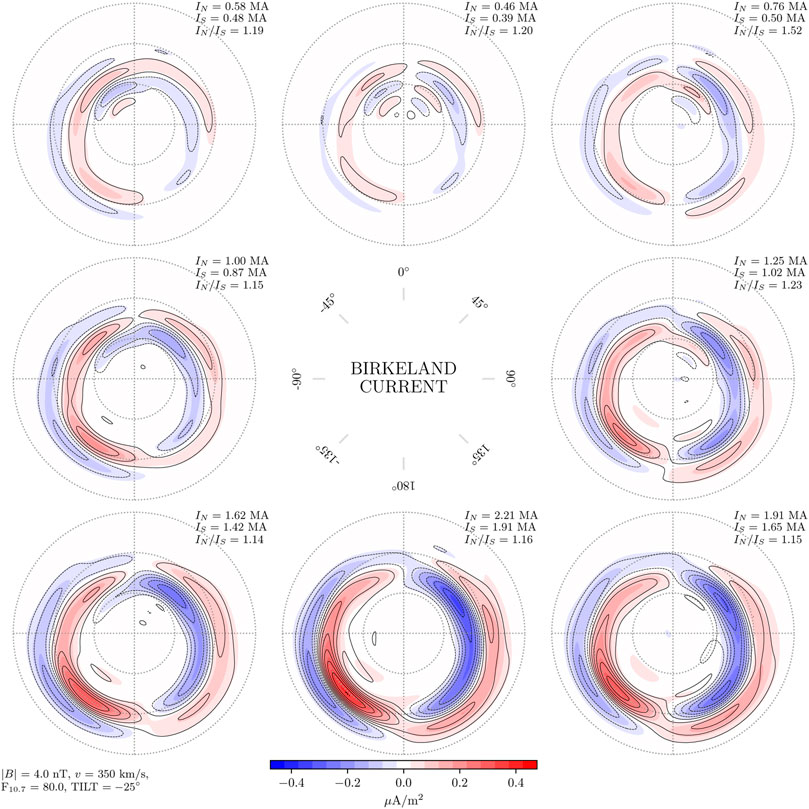
FIGURE 2. Amplitude of Birkeland currents in the Northern Hemisphere (colored contours) and Southern Hemisphere (black contour lines) as a function of IMF clock angle for dipole tilt angle ψ = − 25°, where the signs of By and ψ are reversed for the Southern Hemisphere. The spacing between both contours and contour lines is 0.05μA/m2. In this figure, the mean hemispherically integrated current (top right corner of each panel) in the Northern Hemisphere is 18% stronger than in the Southern Hemisphere.
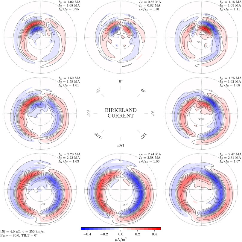
FIGURE 3. Amplitude of Birkeland currents in the Northern Hemisphere (colored contours) and Southern Hemisphere (black contour lines) for dipole tilt angle ψ = 0°, in the same layout as Figure 2. In this figure the mean hemispherically integrated current in the Northern Hemisphere is 4% stronger than in the Southern Hemisphere.
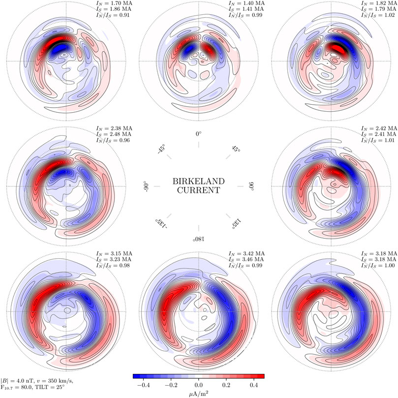
FIGURE 4. Amplitude of Birkeland currents in the Northern Hemisphere (colored contours) and Southern Hemisphere (black contour lines) for dipole tilt angle ψ = 25°, in the same layout as Figure 2. In this figure, the mean hemispherically integrated current in the Northern Hemisphere is 2% weaker than in the Southern Hemisphere.
Figures 2–4 all show that the current density contours are closely aligned in the two hemispheres. This shows that for the Birkeland current density, j(λ, By, ψ, … ) = j(−λ, −By, −ψ, … ) is a good approximation for BT = 4 nT and solar wind speed vx = −350 km/s. The most promwinent deviation from symmetry is seen during local winter (Figure 2), where current densities are stronger in the Northern Hemisphere than in the Southern Hemisphere for all IMF orientations. On average the integrated total Birkeland current J = |J↑| + |J↓| is 18% stronger in the north.
Examination of the difference of the northern and southern contours for each IMF orientation during local winter (not shown) indicates that the imbalance is primarily on the nightside, where northern Birkeland current densities are stronger. Regarding the other dipole orientations, local summer and equinox, the differences of current densities in the two hemispheres (not shown) appear to be mostly controlled by the orientation of IMF By. For example, under positive IMF By in the north (negative in the south) the largest hemispheric differences in Birkeland currents are on the dawnside, while for negative IMF By in the north (positive in the south) the largest differences are on the duskside.
As described above, Figures 2–4 correspond to a particular set of solar wind and IMF conditions (BT = 4 nT and vx = −350 km/s). Two general questions therefore arise: 1) How does the hemispheric difference in total Birkeland current vary with solar wind and IMF conditions? 2) How does the symmetry between the distributions of Birkeland current densities in each hemisphere vary with solar wind and IMF conditions?
To answer the first question, the top row of Figure 5 shows the north/south ratio of integrated total Birkeland current for dipole tilt angles − 25°, 0°, and 25° (panels from left to right), as a function of IMF clock angle θc and the product
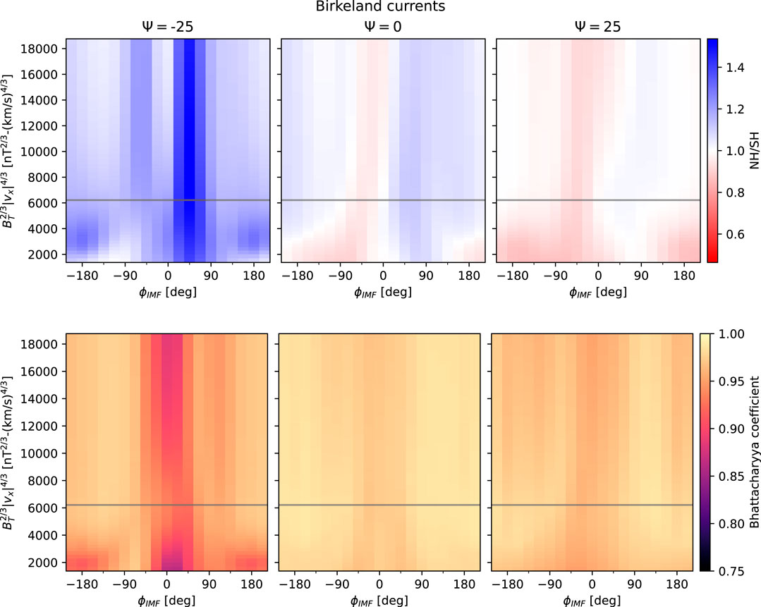
FIGURE 5. Northern and southern total Birkeland current ratio (top row) and Bhattacharyya coefficient (bottom row) as a function of IMF clock angle θc and
To answer the second question, we use the Bhattacharyya coefficient BC to measure the degree of similarity between pairs of Birkeland current distributions in each hemisphere. This coefficient is a measure of the degree of similarity of two probability distributions. It varies from 0, corresponding to distributions with no overlap, to 1, corresponding to distributions that are identical. The definition of BC, as well as our method for calculating it for a given set of northern and southern Birkeland current distributions, is described in the Appendix A.
The bottom row of Figure 5 shows BC in the same layout as the top row. In general BC is high
3.2 Divergence-free equivalent currents
Figures 6–8 show contours that represent the divergence-free current function. The divergence-free current in the AMPS model is estimated with magnetic field measurements made from low Earth orbit, but it is similar to the equivalent current that can be estimated from ground magnetometers. A fixed amount of (divergence-free) current, 10 kA, flows between the contours, so that the current density is proportional to the gradient of the current function. The current direction is rotated 90° clockwise to the gradient, and the gradient is positive in the direction from dashed to solid contours.
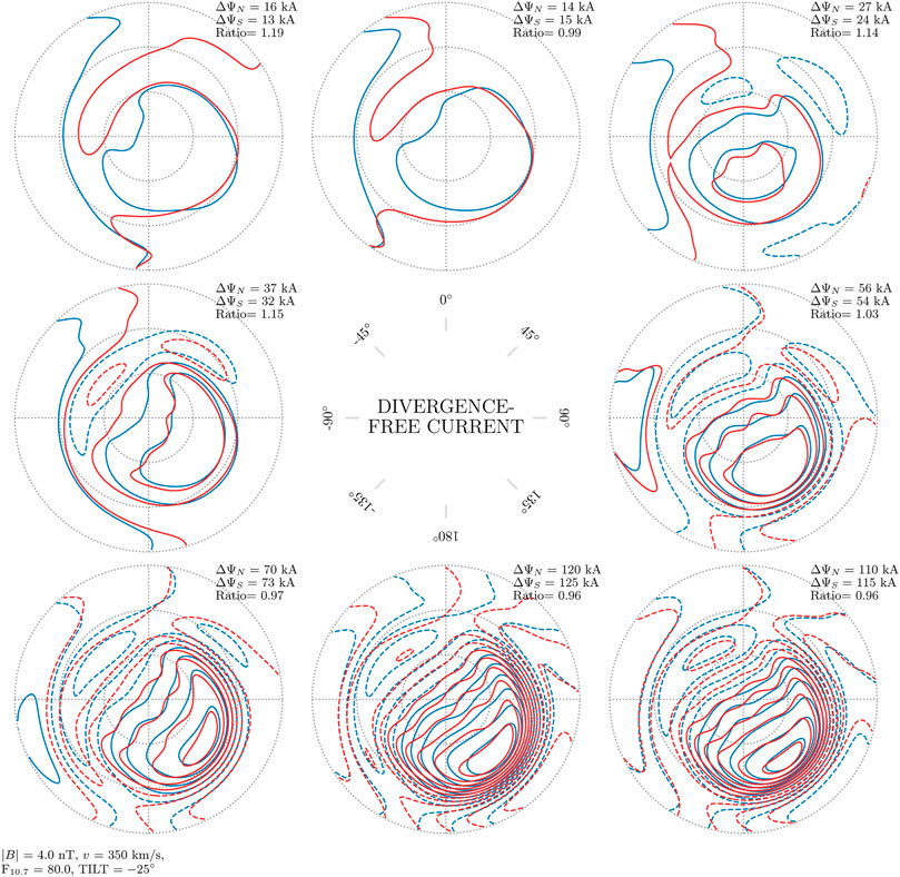
FIGURE 6. Divergence-free current function in the Northern and Southern Hemisphere (blue and red contours, respectively), as a function of IMF clock angle for dipole tilt angle ψ = −25°, where the signs of By and ψ are reversed for the Southern Hemisphere. The spacing between contours is 10 kA. In this figure, the mean of the total currents in the Northern Hemisphere differs from the mean total current in the Southern Hemisphere by less than 1%.
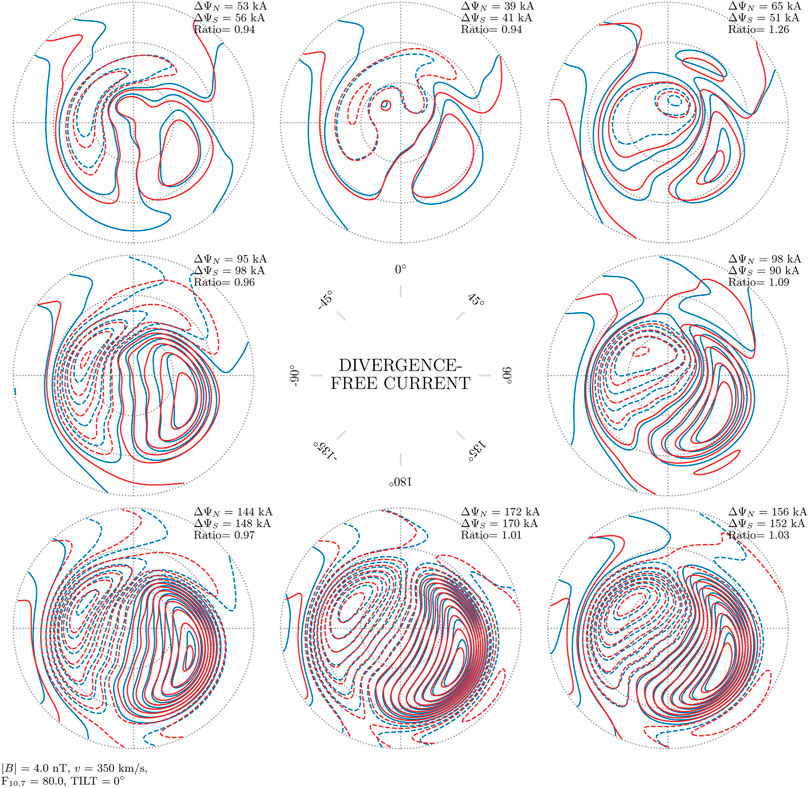
FIGURE 7. Divergence-free current function in the Northern and Southern Hemisphere as a function of IMF clock angle for dipole tilt angle ψ = 0°, in the same format as Figure 6. In this figure, the mean of the total currents in the Northern Hemisphere is 2% stronger than the mean total current in the Southern Hemisphere.
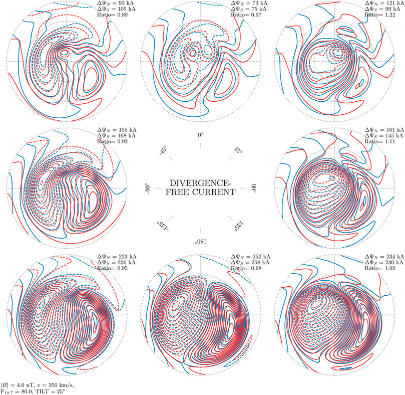
FIGURE 8. Divergence-free current function in the Northern and Southern Hemisphere as a function of IMF clock angle for dipole tilt angle ψ = 25°, in the same format as Figure 6. In this figure, the mean of the total currents in the Northern Hemisphere differs from the mean total current in the Southern Hemisphere by less than 1%.
There are only very subtle differences between the current contours from the two hemispheres in all panels of Figures 6–8. In these three figures the largest mean difference in total current, the current that flows between maximum and minimum of the current function, is only 2%. We conclude that for the average divergence-free current, j(λ, By, ψ, … ) = j( − λ, − By, − ψ, … ) is a good approximation. At the same time it is clear that for individual IMF orientations the difference can be large (e.g., top-left and top-right panels of Figure 6 corresponding to (Bz > 0, By < 0) and (Bz > 0, By > 0), where total current in the two hemispheres differs by factors of 1.19 and 1.14).
Figure 9 summarizes both the variation of the hemispheric difference in total divergence-free current (top row) and the Bhattacharyya coefficients (i.e., overall degree of symmetry) for northern and southern distributions of divergence-free currents (bottom row), in the same layout as Figure 5.
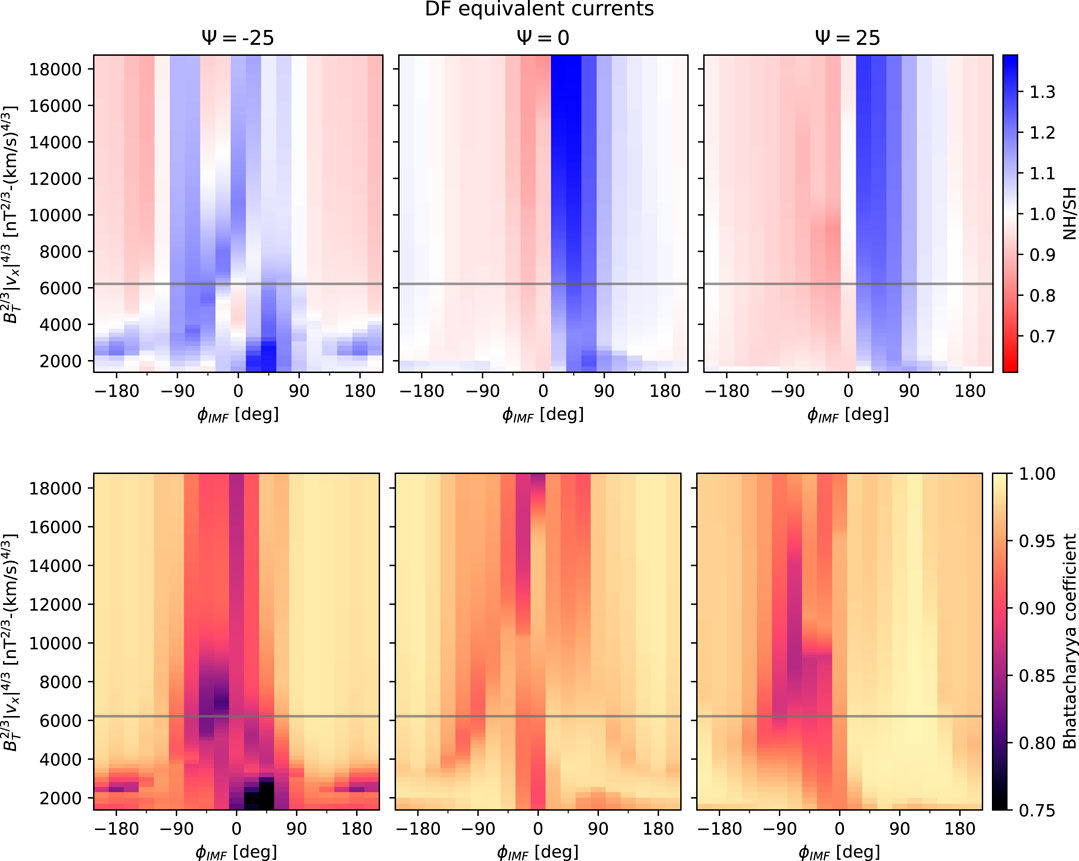
FIGURE 9. Northern and southern total divergence-free current ratio (top row) and Bhattacharyya coefficient of divergence-free current distributions (bottom row) in the same layout as Figure 5.
The north-south ratio of total divergence-free current values in each hemisphere (top row of Figure 9) shows a trend similar to that seen for the integrated total Birkeland currents (top row of Figure 5), namely that the southern equivalent current tends to be greatest for By < 0, and the northern equivalent current tends to be greatest for By > 0. These general trends are not observed for ψ = −25°.
Comparing the Bhattacharyya coefficients for the divergence-free current functions in each hemisphere (bottom row) with those of the Birkeland current distributions (bottom row of Figure 5) indicates that the degree of similarity of the diverge-free current functions is overall lower than that of the Birkeland current distributions, and is generally lowest for dipole tilt ψ = −25°. Even so, the minimum and mean values of BC for ψ = −25° (0.73 and 0.95) are still relatively high.
3.3 Comparison with Coxon et al. (2016)
The high degree of symmetry found in Figures 2–4 appears to contradict the results of Coxon et al. (2016), who report significantly stronger currents in the Northern Hemisphere than in the Southern, based on the Active Magnetosphere and Planetary Electrodynamics Response Experiment (AMPERE) (Anderson et al., 2000; Waters et al., 2001). AMPERE uses platform magnetometers onboard the fleet of Iridium® satellites to provide estimates of Birkeland currents in both hemispheres in 10-min windows every 2 min. In this section we use an extended AMPERE data set together with the methodology presented by Coxon et al. (2016) for quantifying the overall hemispheric difference in integrated Birkeland current intensity, and compare with corresponding estimates using the AMPS model. Our goal is to determine whether Birkeland currents as represented by the AMPS model evince a clear preference for the Northern Hemisphere, similar to that observed with the AMPERE data set.
Coxon et al. (2016) used Iridium®-based estimates of the Birkeland currents to calculate the total current into and out of each hemisphere, and then calculated 27-day (one Bartels rotation) averages for a period of 6 years (2010–2015). To examine the difference in current throughput through each hemisphere, they posited that the Birkeland currents roughly follow a kind of global Ohm’s law,
where J = |J↑| + |J↓| is the total Birkeland current,
is a function that plays the role of conductance with t = 2π(d − 79)/365.25, and d the number of days since 1 January 2010. The coefficients c1 and c2 are intended to represent the “background conductance” and “the variation in conductance due to seasonal effects.” The Milan et al. (2012) coupling function
estimates the total dayside reconnection rate and has units of kV, or equivalently kWb/s (magnetic flux per time). In this expression the transverse IMF component BT is given in T and vx in km/s, and RE is the radius of Earth in km. Coxon et al. (2016) justify their use of Eq. 2 by pointing to the study of Coxon et al. (2014), who find that J and ΦD are highly correlated, and observing that the factor relating J and ΦD (Ξ) has units of conductance.
Following Coxon et al. (2016), we seek to obtain the best-fit values of c1 and c2 in Eq. 3 for both the AMPERE and AMPS hemispheric total currents in Figure 10A. To calculate the hemispherically integrated total Birkeland current from the AMPS model in each hemisphere, we first smooth the relevant solar wind and IMF parameters (solar wind speed vx and IMF By and Bz) from the OMNI database (King and Papitashvili, 2005) with a 20-min rolling window and calculate the 27-days average of the F10.7 index, and use these averaged parameters together with dipole tilt as input to AMPS. We then calculate the model Birkeland current for all MLats
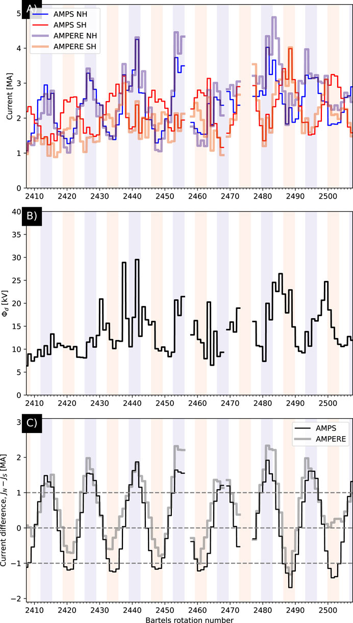
FIGURE 10. Comparison of the total field-aligned current in the two hemispheres and between our model and AMPERE, as a function of Bartels rotation number (number of 27-day periods since 8 February 1832). (A) Thick lines indicate AMPERE currents, and thin lines indicate AMPS model currents. Northern and Southern Hemisphere lines are indicated in blue and red, respectively. The red and blue shades in the background indicate the three months around June (blue) and December (red). (B) Dayside reconnection rate, in kV, using the (Milan et al., 2012) coupling function. (C) The difference in total current between hemispheres. The format of this figure is similar to that of Figure 3a in Coxon et al. (2016).
We then perform a fit to the expression Ξ(t) = J/ΦD using J and ΦD from panels A and B, respectively, in Figure 10, which yields the fit values for c1 and c2 shown in Table 1. Coxon et al. (2016) found that c1,N/c1,S = 202.6/154.4 ≈ 1.3, and c2,N/c2,S = 54.0/ −50.6 ≈ −1.1. The ratio of their c1 coefficients indicates that the baseline of the conductance-like function Σ is greater by ∼30% in the Northern Hemisphere, while their ratio of c2 coefficients indicates 1) slightly greater seasonal variation of Σ in the Northern Hemisphere, and 2) an unsurprising phase difference of approximately half a year in hemispheric variations.
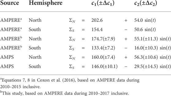
TABLE 1. Global conductances estimated from Eq. 3.
For the slightly extended AMPERE data set that we have used, Table 1 shows that c1,N/c1,S = 174.7/133.4 ≈ 1.3 and c2,N/c2,S = 55.1/ −16 ≈ −3.4. In other words, our extended AMPERE data yields a result very similar to that of Coxon et al. (2016) for the baseline c1 coefficients. On the other hand we find a substantially weaker seasonal variation (represented by c2 coefficients) for the Southern Hemisphere.
Turning to AMPS data, c1,N/c1,S = 160/146 ≈ 1.1 and c2,N/c2,S = 56.3/ −29.5 ≈ −1.9. Thus we also find a baseline “global conductance” that is greater in the Northern Hemisphere, although the difference is only 10% instead of 30%. We also find that the seasonal variation is nearly twice as great in the Southern Hemisphere, relative to the extended AMPERE-based c2 coefficient.
Apart from this fit-based comparison, Figure 10C shows the difference in hemispheric currents in Figure 10A for AMPERE (thick gray line) and the AMPS model (thin black line). Throughout the time series the AMPERE-derived hemispheric current difference tends to have higher peaks than troughs, indicating that according to AMPERE data the Northern Hemisphere total current is greater than that in the Southern. The AMPS-derived hemispheric current difference is generally more centered around zero. To be specific, the averages of the AMPERE and AMPS JN − JS time series in Figure 10C are respectively 0.56 and 0.13 MA. The offset of this time series in favor of the Northern Hemisphere as shown in Figure 2 of Coxon et al. (2016) is even more extreme, with the peak and trough typically greater than 2 MA and less than -1 MA, respectively.
4 Discussion
The main conclusions from the preceding analysis of hemispheric differences in Birkeland and divergence-free currents are the following.
1. For both Birkeland and divergence-free horizontal currents, the total currents more or less exhibit mirror symmetry during local equinox and local summer (Ψ = 0° and Ψ = 25° in the NH, respectively) when averaged over IMF clock angle orientation. During local winter (Ψ = −25° in the NH) the two types of currents display different behaviors: For the Birkeland currents, NH total current tends to dominate regardless of IMF clock angle orientation; for the divergence-free currents, NH total current tends to dominate for Bz > 0 and
2. The NH/SH ratio of total Birkeland current exhibits a slight overall dependence on dipole tilt, whereby the NH dominates during local winter (average NH/SH ratio of 1.17 for all values shown in the top left panel of Figure 5), as previously mentioned, and the SH exhibits very slight dominance over the NH during local summer average NH/SH ratio of 0.98 for all values shown in the top right panel of Figure 5).
3. With respect to dependence on IMF orientation, both Birkeland and divergence-free currents display a higher degree of mirror symmetry for Bz < 0 than for Bz > 0 (Figures 5, 9), regardless of the orientation of By. On the other hand, for Bz > 0, NH total current tends to be favored for By > 0 in the NH and By < 0 in the SH, while SH total current tends to be favored for By < 0 in the NH and By > 0 in the SH.
Regarding the overall higher degree of symmetry exhibited by total Birkeland and divergence-free currents in each hemisphere for Bz < 0 relative to Bz > 0, Workayehu et al. (2021) draw essentially the same conclusion using Swarm satellite measurements, but a rather different methodology based on spherical elementary currents. Regarding the overall variation of the NH/SH ratio of total Birkeland current with season, Workayehu et al. (2020) also find that NH total Birkeland current is greater by about 20% during local winter. Workayehu et al. (2021) also find that NH/SH ratio of total Birkeland current is greatest, 1.2 ± 0.09, for Bz > 0 and By > 0 in the NH (By < 0 in the SH) during local winter, although we find that the NH/SH ratio is overall greater, between 1.3 and 1.55 for this IMF orientation. Last, Workayehu et al. (2021) also find that the total Birkeland current during local summer is slightly less in the NH than in the SH for all IMF conditions, with an average ratio of 0.94 (their Table 2). On the other hand, while we find very little average difference in divergence-free current between hemispheres during local winter (less than 1%), Workayehu et al. (2020) find that Northern Hemisphere divergence-free currents are about 10% stronger.
We have also carried out a detailed comparison of seasonal variations in Birkeland currents as represented by AMPS and AMPERE data. While we, like Coxon et al. (2016), find that the Northern Hemisphere Birkeland currents are larger than those in the Southern Hemisphere, the difference we find is more modest, and more in line with the differences of order 10–20% that are shown in Figures 2–4. One possible explanation for the overall higher degree of hemispheric symmetry in the Birkeland currents that we find relative to the results of Coxon et al. (2016) is that, for earlier versions of AMPERE data processing, the Southern Hemisphere estimates of the field-aligned current reportedly sometimes include spurious filamentary currents at the high-latitude orbit crossing (Anderson et al., 2017). Additionally, at present, field-aligned currents derived from Iridium®satellite measurements up to and including 2017 sometimes underestimate Birkeland current magnitudes in the Southern Hemisphere. This underestimate is addressed and rectified in an upcoming release of AMPERE data [private communication, C. L. Waters, 2022].
As a result of the high
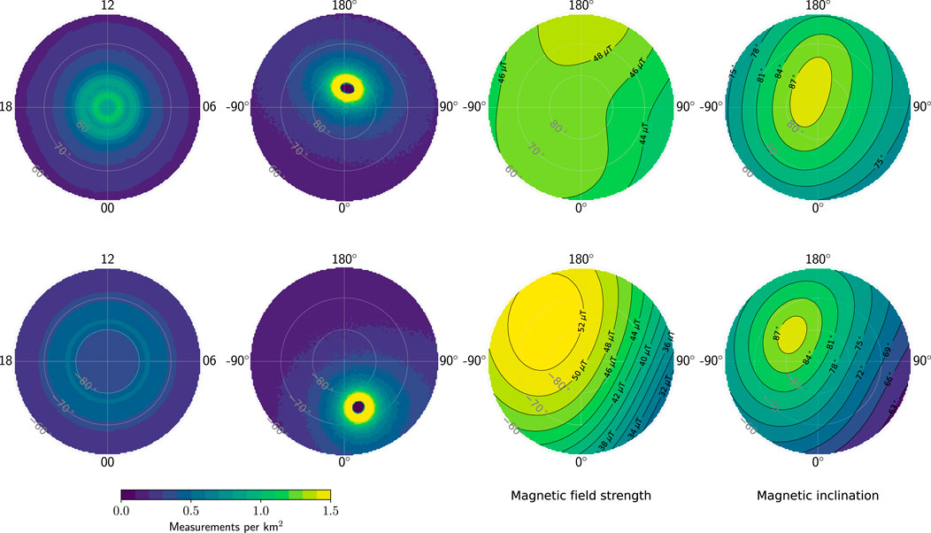
FIGURE 11. Color plots of the distributions of data points used to make the AMPS model in the Northern and Southern Hemisphere (top and bottom row, respectively), shown on a magnetic latitude-local time grid (column one) and magnetic latitude-longitude grid (column two). Also shown are the magnetic field strength (column three) and the inclination angle (column four), evaluated at 450-km altitude using the IGRF model.
On the other hand, methodological differences for deriving statistics from AMPERE and Swarm data could possibly explain how we arrive at somewhat different results. AMPERE statistics are averages of global maps that are each based on 10 min of data, such that the nonuniformity in sampling is included in every such map (e.g., Figure 1 in Waters et al., 2001). AMPS statistics are instead produced by first deriving a model from data on an MLat-MLT grid collected over several years (column one of Figure 11), and then querying the model. While quantifying the effect of these methodological differences would require a dedicated study, our intention here is to point out that it seems reasonable to think that these methodological differences could play a role. Some of these points have been raised by Green et al. (2009), who also report an overall hemispheric difference in Birkeland currents on the basis of AMPERE measurements. They attribute the difference to the satellite orbits, the relatively greater displacement of the magnetic pole from the geographic pole in the Southern Hemisphere, and the unavailability of the along-track component of magnetic field measurements.
Regardless of these possible explanations, we are confident in the AMPS-based results as the AMPS model was designed to account for what we term the “direct effects” of local distortions of the geomagnetic field and the nonorthogonality of coordinate systems based on the geomagnetic field. Hemispheric and longitudinal variations in the main magnetic field, for example, has a direct geometric effect on the current density: For a constant incident current at some absolute magnetic latitude and local time, the observed current density is proportional to the magnetic field strength. This is because as the magnetic field lines converge with decreasing altitude, they focus the same current on a smaller area where the field is strong compared to regions with weaker magnetic field. This geometric effect is taken into account in the AMPS model by virtue of its use of Apex coordinates.
To illustrate this point more concretely we refer to the magnetic field strength shown on MLat-MLon grids in each hemisphere in column three of Figure 11. At 70° MLat and 90° MLon, for example, the magnetic field strengths in the Northern and Southern Hemisphere are approximately 44 and 40 μT, respectively. The difference in magnetic field strengths at these conjugate points therefore imply, for the same total incident current, that the measured current density would be 10% stronger in the Northern hemisphere. Closer to the pole the hemispheric asymmetry in field strength is reversed. But since field-aligned currents tend to be weak in the polar cap, we would expect that for the same total current flowing into each hemisphere, the total current would appear stronger in the north in statistical studies that do not take the geometric effects related to field strength into account. Such effects could explain some of the difference between statistics based on AMPS and other statistics.
4.1 Possible influence of longitudinal variations in field strength and inclination
Beyond the direct effects of geomagnetic field distortion, there are also indirect effects that are not accounted for in the AMPS model. These include the non-trivial dependence of ionospheric conductance and currents on the geomagnetic field strength and inclination (Gasda and Richmond, 1998). Here we attempt to outline the possible influence of such effects.
To fully understand the differences between ionospheric current systems in each hemisphere, it is not enough to compare features at conjugate magnetic local times, as we have done with Figures 2–8. The reason is that the orientation of the MLat-MLT grid, and the solar zenith angle of points on the grid, varies throughout the day—that is, the geometry of the grid with respect to incident sunlight depends on Universal Time (UT), see Figure 1. The geomagnetic field strength and inclination are, however, functions of MLon rather than MLT (columns three and four, respectively, in Figure 11). Therefore, the nonuniformity of the sampling distribution on the MLat-MLon grid is mapped via UT onto the MLat-MLT grid on which the AMPS model is derived, in such a way that some magnetic field strengths and inclinations are sampled more often than others at a given MLat and MLT.
Short of adding UT as a AMPS model parameter, which would address this issue, we can instead determine the degree of bias toward a particular magnetic field strength and inclination inherent in the distribution of measurements used to construct the AMPS model. We do this by weighting the distributions of magnetic field strength and inclination in each hemisphere (third and fourth columns, respectively, in Figure 11) by the corresponding sampling density distributions (second column in Figure 11), and then integrating these weighted distributions around rings of constant QD latitude to obtain marginal distributions of magnetic field strength and inclination (left and right panels in Figure 12) in the Southern (red) and Northern (blue) Hemispheres. The marginal distributions based on the sampling distributions (solid lines) are shown together with reference marginal distributions (dotted lines) for which all magnetic latitudes and longitudes are weighted equally.
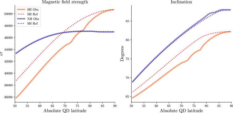
FIGURE 12. Marginal distributions of geomagnetic field strength (left) and field inclination (right) in the Northern (blue) and Southern (red) Hemisphere for the sampling distribution used to create the AMPS model (solid lines, denoted ”Obs”) and for a reference uniform distribution (dotted lines, denoted ”Ref”). Solid lines are obtained by weighting the field strength and inclination in each hemisphere with the corresponding sampling distribution and integrating over longitude, while dotted lines are obtained by instead weighting with a uniform distribution.
Comparing the sampling and reference Northern Hemisphere marginal distributions, we see that the two match closely, indicating that little bias is present in the AMPS model with respect to Northern Hemisphere magnetic field strength and inclination. Making the same comparison with the Southern Hemisphere curves, we see that the field strength of the sample distribution is typically about 8% less than that of the reference distribution except toward the pole, where the two lines must converge. The reason is that at the SH geographic pole, around which the Swarm satellite sampling density is heavily concentrated (second row, bottom panel in Figure 11), the main field strength is weaker than it is at the SH geomagnetic pole (third row, bottom panel in Figure 11). For the same reason, the inclination of the sampling distribution is one or two degrees below that of the reference distribution for all latitudes except near the pole.
To illustrate why these biases in sampled field strength and field inclination could be important, we insert the value of the ratio B0,Obs/B0,Ref ( = 40 μT /44 μT = 0.93) from the Southern Hemisphere curves at
4.2 Comparison with particle precipitation
In Section 3 we found that the average integrated Birkeland current during local winter (Figure 2) is 18% stronger in the Northern Hemisphere, primarily on the nightside, with the proviso that the distribution of measurements used to derive the AMPS model is biased in magnetic latitude-longitude. We now examine whether a north-south asymmetry is also observed in particle precipitation statistics, subject to the same bias in magnetic latitude-longitude sampling as AMPS and with the bias removed. We accomplish this using electron precipitation data from the full Fast Auroral SnapshoT mission, covering the period from November 1996 through April 2009. This database is publicly available (Hatch, 2022).
Following a methodology similar to that of Chaston et al. (2007) and Hatch et al. (2016), we calculate the electron current density and energy flux inside the earthward loss cone and above 70 eV up to the 30-keV detector limit. The 70-eV lower limit is used to avoid contamination from spacecraft charging. We then map these measurements along IGRF magnetic field lines from the satellite to a height of 110 km by scaling each measurement by the ratio of the magnetic field strength at these two heights. Since we are interested in local winter, we select measurements from the Northern Hemisphere for which the dipole tilt angle ψ ≤ −20°, and measurements from the Southern Hemisphere for which the dipole tilt angle ψ ≥ 20°. Of a total of 44.4 million total measurements in the FAST precipitation database, for these conditions and for Modified Apex-110 latitudes at or above 60° there are 26.5 million measurements in the Northern Hemisphere and 26.1 million in the Southern. In survey mode, the typical cadence of the FAST electron electrostatic analyzer (EESA) instrument
The orbit of FAST is, like those of Swarm and AMPERE, polar, and the distribution of measurements on a magnetic latitude-longitude grid (not shown) is very similar to that of the Swarm satellites (column two in Figure 11). Therefore the FAST measurements are biased in longitude in the same way as Swarm measurements. Integrating the distributions of mean current density in column two of Figure 13, we find that the longitude-biased Northern Hemisphere integrated current density is 15% greater than that of the Southern Hemisphere. This is rather comparable to the 18% difference we find with AMPS. Performing the same calculation for the longitude-biased mean energy flux (column four of Figure 13) we find that the longitude-biased Northern Hemisphere integrated energy flux is 3% less than that of the Southern Hemisphere. The only possible explanation for this apparent discrepancy is that the Southern Hemisphere electrons are, on average, more energetic than those in the North during local winter. Incidentally, the reason for the much higher typical current densities seen in columns two and three of Figure 13 relative to those in Figures 2–4 is that the former represent a moment of the observed distribution function that is calculated based on a limited range of pitch angles (i.e., only those within the earthward portion of the loss cone) and energies (0.07–32 keV). This moment excludes any electrons outside these ranges, including all anti-earthward electrons. Distributions of loss-cone current density and energy flux are moreover logarithmic (not shown, but see, e.g., Figure 3 of Hatch et al. (2016)), which means that large current densities greatly influence the mean of any collection of samples of such measurements.
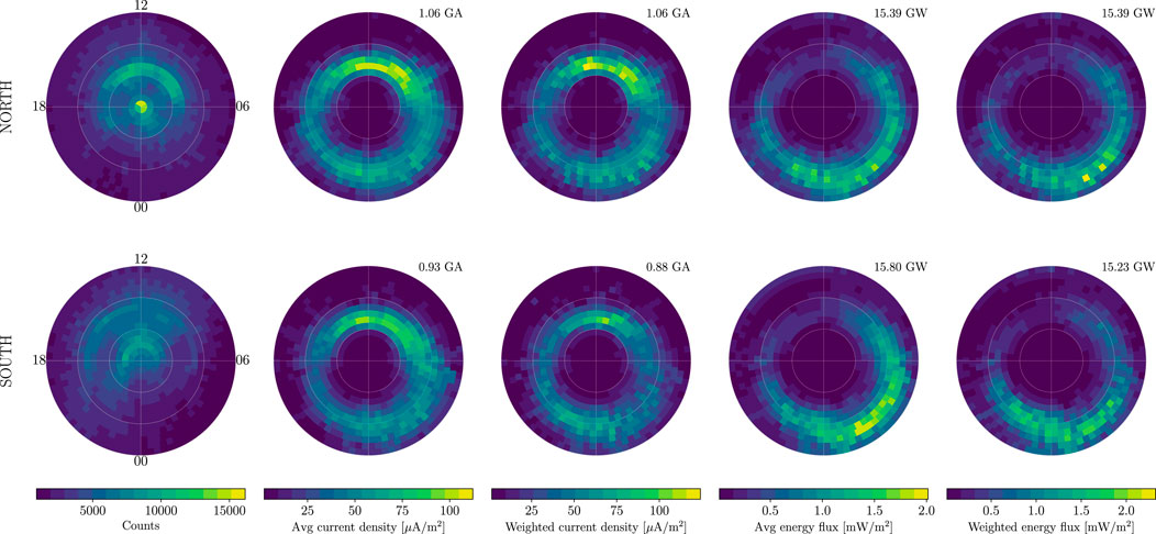
FIGURE 13. FAST electron loss-cone precipitation statistics in the Northern and Southern Hemisphere (top and bottom row, respectively) during local winter. The first column shows the number of measurements in each hemisphere. The second and third columns show the longitude-biased and unbiased average current density, respectively. The fourth and fifth columns show the longitude-biased and unbiased average energy flux. Statistics are calculated on an approximately equal-area MLat-MLT grid.
To remove the magnetic longitude sampling bias from these estimates, we calculate a weighted average of the current density and energy flux in each hemisphere (columns three and five of Figure 13), where each measurement is first weighted by the inverse of the number of measurements where that measurement occurs on a magnetic latitude-longitude grid. The effect that this weighting has most clearly seen by comparing the distribution of energy flux in the Southern Hemisphere based on a simple average with that of the weighted average (bottom panel in the fourth and fifth columns, respectively, of Figure 13). Removing the longitude bias visibly reduces the average energy flux between approximately 60° and 70° MLat and 0–6 MLT.
Integrating the distributions of mean number flux in column three of Figure 13, we find that the unbiased Northern Hemisphere integrated number flux is 20% greater than that of the Southern Hemisphere, which is also comparable to the 18% difference we find with AMPS. Performing the same calculation for the unbiased average energy flux (column five of Figure 13) we find that the unbiased Northern Hemisphere integrated energy flux is 1% greater than that of the Southern Hemisphere. Therefore, removing the longitude bias does not change the conclusion based on the longitude-biased estimates that the Southern Hemisphere electrons observed by FAST must be, on average, more energetic than those observed in the North during local winter over the range of energies measured by the FAST EESA.
AMPS- and FAST-based results therefore appear to corroborate one another. FAST observations additionally indicate that the net electron energy flux into each hemisphere during local winter is approximately equal. We reserve a full investigation of the possible hemispheric differences in current input and energy input for a future study.
5 Conclusion
In summary, we have used the Swarm-based AMPS model of Birkeland and ionospheric divergence-free currents in both hemispheres to quantify how much they depart with the commonly employed mirror symmetry assumption. We have highlighted that the AMPS model is particularly well suited to this test as it is designed to take stock of what we have termed the “direct effects” of the nonorthogonal nature of coordinate systems based on the geomagnetic field. We find that under a reversal of the sign of the dipole tilt angle and IMF By in the Southern Hemisphere, the morphology of Birkeland and divergence-free current distributions in each hemisphere are highly similar, with mean Bhattacharyya coefficients of respectively 0.97 and 0.96 for all solar wind driving and IMF clock angle conditions that we have considered. (Without performing this reversal of the sign of dipole tilt angle and IMF By the mean Bhattacharyya coefficients are 0.78 and 0.74, respectively.) We also find that on average, the total Birkeland and ionospheric divergence-free currents are similar with mean NH/SH total current ratios of 1.06 and 1.02 for Birkeland and divergence-free currents for all solar wind driving and IMF clock angle conditions considered. In general, differences between total currents in the two hemispheres are strongest during Bz > 0, with By > 0 in the NH (By < 0 in the SH) tending to favor the NH, and By < 0 in the NH (By > 0 in the SH) tending to favor the SH, in accordance with earlier studies (e.g., Workayehu et al., 2021). We have also compared our results with those of Coxon et al. (2016), and find that our results indicate a relatively higher degree of hemispheric symmetry. The largest exception appears to be the Birkeland currents during local winter, when the average difference in integrated currents is approximately 20%, which is in accordance with the results of Workayehu et al. (2020). FAST satellite observations from each hemisphere during local winter corroborate this result, but additionally indicate that the net electron energy input into each hemisphere during local winter is the same within a few percent.
Data availability statement
The original contributions presented in the study are included in the article/Supplementary Material, further inquiries can be directed to the corresponding author.
Author contributions
SH contributed to data analysis and interpretation, study design, and manuscript preparation. KL contributed to data analysis and interpretation, study design, and manuscript preparation. JR contributed to manuscript preparation and data interpretation.
Funding
This work was supported by the Trond Mohn Foundation and by the Research Council of Norway under contracts 223252/F50 and 300844/F50. The study is also funded by ESA through the Swarm Data Innovation and Science Cluster (Swarm DISC) within the reference frame of ESA contract 000109587/13/I-NB. For more information on Swarm DISC, please visit https://earth.esa.int/web/guest/missions/esa-eo-missions/swarm/disc.
Acknowledgments
We thank ESA for providing prompt access to the Swarm L1b data. The support of the CHAMP mission by the German Aerospace Center (DLR) and the Federal Ministry of Education and Research is gratefully acknowledged. The IMF, solar wind and magnetic index data were provided through OMNIWeb by the Space Physics Data Facility(SPDF). We also thank the AMPERE team and the AMPERE Science Center for providing the Iridium®-derived data products.
Conflict of interest
The authors declare that the research was conducted in the absence of any commercial or financial relationships that could be construed as a potential conflict of interest.
Publisher’s note
All claims expressed in this article are solely those of the authors and do not necessarily represent those of their affiliated organizations, or those of the publisher, the editors and the reviewers. Any product that may be evaluated in this article, or claim that may be made by its manufacturer, is not guaranteed or endorsed by the publisher.
Appendix A:
To calculate the Bhattacharyya coefficient for a pair of northern and southern Birkeland current distributions (or divergence-free equivalent current distributions), we must first convert each current distribution, which can be positive or negative, to a continuous probability distribution with only positive values. Each distribution j = j(λ, ϕMLT), with
and
We then normalize the probability distribution j∗ such that
After following the above procedure to obtain probability distributions
References
Anderson, B. J., Korth, H., Welling, D. T., Merkin, V. G., Wiltberger, M. J., Raeder, J., et al. (2017). Comparison of predictive estimates of high-latitude electrodynamics with observations of global-scale birkeland currents. Space weather. 15, 352–373. doi:10.1002/2016SW001529 |
Anderson, B. J., Takahashi, K., and Toth, B. A. (2000). Sensing global Birkeland currents with Iridium engineering magnetometer data. Geophys. Res. Lett. 27, 4045–4048. doi:10.1029/2000gl000094 |
Andreeva, V. A., and Tsyganenko, N. A. (2016). Reconstructing the magnetosphere from data using radial basis functions. JGR. Space Phys. 121, 2249–2263. doi:10.1002/2015JA022242 |
Avery, S., Vincent, R., Phillips, A., Manson, A., and Fraser, G. (1989). High-latitude tidal behavior in the mesosphere and lower thermosphere. J. Atmos. Terr. Phys. 51, 595–608. doi:10.1016/0021-9169(89)90057-3 |
Barlier, F., Bauer, P., Jaeck, C., Thuillier, G., and Kockarts, G. (1974). North-south asymmetries in the thermosphere during the Last Maximum of the solar cycle. J. Geophys. Res. 79, 5273–5285. doi:10.1029/JA079i034p05273 |
Billett, D. D., Grocott, A., Wild, J. A., Walach, M.-T., and Kosch, M. J. (2018). Diurnal variations in global joule heating morphology and magnitude due to neutral winds. J. Geophys. Res. Space Phys. 123, 2398–2411. doi:10.1002/2017JA025141 |
Chaston, C. C., Carlson, C. W., McFadden, J. P., Ergun, R. E., and Strangeway, R. J. (2007). How important are dispersive Alfvén waves for auroral particle acceleration? Geophys. Res. Lett. 34, L07101. doi:10.1029/2006GL029144 |
Clausen, L. B. N., Baker, J. B. H., Ruohoniemi, J. M., Milan, S. E., and Anderson, B. J. (2012). Dynamics of the region 1 birkeland current oval derived from the active magnetosphere and planetary electrodynamics response experiment (AMPERE). J. Geophys. Res. 117. doi:10.1029/2012JA017666 |
Cosgrove, R. B., Bahcivan, H., Chen, S., Sanchez, E., and Knipp, D. (2022). Violation of hemispheric symmetry in integrated poynting flux via an empirical model. Geophys. Res. Lett. 49, e2021GL097329. doi:10.1029/2021GL097329 | |
Cowley, S., and Hughes, W. (1983). Observation of an IMF sector effect in the Y magnetic field component at geostationary orbit. Planet. Space Sci. 31, 73–90. doi:10.1016/0032-0633(83)90032-6 |
Coxon, J. C., Milan, S. E., Carter, J. A., Clausen, L. B. N., Anderson, B. J., and Korth, H. (2016). Seasonal and diurnal variations in AMPERE observations of the Birkeland currents compared to modeled results. J. Geophys. Res. Space Phys. 121, 4027–4040. doi:10.1002/2015JA022050 |
Coxon, J. C., Milan, S. E., Clausen, L. B. N., Anderson, B. J., and Korth, H. (2014). The magnitudes of the regions 1 and 2 Birkeland currents observed by AMPERE and their role in solar wind-magnetosphere-ionosphere coupling. J. Geophys. Res. Space Phys. 119, 9804–9815. doi:10.1002/2014JA020138 |
Crooker, N. U., and Rich, F. J. (1993). Lobe cell convection as a summer phenomenon. J. Geophys. Res. 98, 13403–13407. doi:10.1029/93JA01037 |
Dhadly, M. S., Emmert, J. T., Drob, D. P., Conde, M. G., Aruliah, A., Doornbos, E., et al. (2019). HL-TWiM empirical model of high-latitude upper thermospheric winds. JGR. Space Phys. 124, 10592–10618. doi:10.1029/2019JA027188 |
Dombeck, J., Cattell, C., Prasad, N., Meeker, E., Hanson, E., and McFadden, J. (2018). Identification of auroral electron precipitation mechanism combinations and their relationships to net downgoing energy and number flux. JGR. Space Phys. 123 10064–10089. doi:10.1029/2018JA025749 |
Finlay, C. C., Kloss, C., Olsen, N., Hammer, M. D., Tøffner-Clausen, L., Grayver, A., et al. (2020). The CHAOS-7 geomagnetic field model and observed changes in the South Atlantic Anomaly. Earth Planets Space 72, 156. doi:10.1186/s40623-020-01252-9 | |
Förster, M., and Haaland, S. (2015). Interhemispheric differences in ionospheric convection: Cluster EDI observations revisited. J. Geophys. Res. Space Phys. 120, 5805–5823. doi:10.1002/2014JA020774 |
Gasda, S., and Richmond, A. D. (1998). Longitudinal and interhemispheric variations of auroral ionospheric electrodynamics in a realistic geomagnetic field. J. Geophys. Res. 103, 4011–4021. doi:10.1029/97JA03243 |
Green, D. L., Waters, C. L., Anderson, B. J., and Korth, H. (2009). Seasonal and interplanetary magnetic field dependence of the field-aligned currents for both Northern and Southern Hemispheres. Ann. Geophys. 27, 1701–1715. doi:10.5194/angeo-27-1701-2009 |
Gussenhoven, M. S., Hardy, D. A., and Heinemann, N. (1983). Systematics of the equatorward diffuse auroral boundary. J. Geophys. Res. 88, 5692. doi:10.1029/JA088iA07p05692 |
Haaland, S., Lybekk, B., Maes, L., Laundal, K., Pedersen, A., Tenfjord, P., et al. (2017). North-south asymmetries in cold plasma density in the magnetotail lobes: Cluster observations. J. Geophys. Res. Space Phys. 122, 136–149. doi:10.1002/2016JA023404 |
Hardy, D. A., Gussenhoven, M. S., and Holeman, E. (1985). A statistical model of auroral electron precipitation. J. Geophys. Res. 90, 4229. doi:10.1029/JA090iA05p04229 |
Hatch, S. M., Chaston, C. C., and LaBelle, J. (2016). Alfvén wave-driven ionospheric mass outflow and electron precipitation during storms. J. Geophys. Res. Space Phys. 121, 7828–7846. doi:10.1002/2016JA022805 |
Hatch, S. M., Haaland, S., Laundal, K. M., Moretto, T., Yau, A. W., Bjoland, L., et al. (2020). Seasonal and hemispheric asymmetries of F region polar cap plasma density: Swarm and CHAMP observations. J. Geophys. Res. Space Phys. 125. doi:10.1029/2020JA028084 |
Hatch, S. M., LaBelle, J., and Chaston, C. (2018). Storm phase–partitioned rates and budgets of global Alfvénic energy deposition, electron precipitation, and ion outflow. J. Atmos. Solar-Terrestrial Phys. 167, 1–12. doi:10.1016/j.jastp.2017.08.009 |
Heppner, J. P., and Maynard, N. C. (1987). Empirical high-latitude electric field models. J. Geophys. Res. 92, 4467–4489. doi:10.1029/JA092iA05p04467 |
Jørgensen, T. S., Friis-Christensen, E., and Wilhjelm, J. (1972). Interplanetary magnetic-field direction and high-latitude ionospheric currents. J. Geophys. Res. 77, 1976. doi:10.1029/JA077i010p01976 |
Keating, G. M., Mcdougal, D. S., Prior, E. J., and Levine, J. S. (1973). “North-South asymmetry of the neutral exosphere,” in Space research XIII. Editors M. J. Rycroft, and S. K. Runcorn (Berlin: Akademie-Verlag), 327.
King, J., and Papitashvili, N. E. (2005). Solar wind spatial scales in and comparisons of hourly Wind and ACE plasma and magnetic field data. J. Geophys. Res. 110, A02104. doi:10.1029/2004ja010649 |
Knipp, D., Kilcommons, L., Hairston, M., and Coley, W. R. (2021). Hemispheric asymmetries in poynting flux derived from DMSP spacecraft. Geophys. Res. Lett. 48. doi:10.1029/2021GL094781 |
Laundal, K. M., Cnossen, I., Milan, S. E., Haaland, S. E., Coxon, J., Pedatella, N. M., et al. (2017). North-South asymmetries in Earth’s magnetic field - effects on high-latitude geospace. Space Sci. Rev. 206, 225–257. doi:10.1007/s11214-016-0273-0 |
Laundal, K. M., Finlay, C. C., Olsen, N., and Reistad, J. P. (2018). Solar wind and seasonal influence on ionospheric currents from Swarm and CHAMP measurements. J. Geophys. Res. Space Phys. 123, 4402–4429. doi:10.1029/2018JA025387 |
Laundal, K. M., Finlay, C. C., and Olsen, N. (2016a). Sunlight effects on the 3D polar current system determined from low Earth orbit measurements. Earth Planets Space 68, 142. doi:10.1186/s40623-016-0518-x |
Laundal, K. M., Gjerloev, J. W., Ostgaard, N., Reistad, J. P., Haaland, S. E., Snekvik, K., et al. (2016b). The impact of sunlight on high-latitude equivalent currents. J. Geophys. Res. Space Phys. 121, 2715–2726. doi:10.1002/2015JA022236 |
Laundal, K. M., Hatch, S. M., and Moretto, T. (2019). Magnetic effects of plasma pressure gradients in the upper F region. Geophys. Res. Lett. 46, 2355–2363. doi:10.1029/2019GL081980 |
Laundal, K. M., and Toresen, M. (2018). pyAMPS. Available at: https://github.com/klaundal/pyAMPS. doi:10.5281/zenodo.1182930 |
Lockwood, M., Owens, M. J., Barnard, L. A., Watt, C. E., Scott, C. J., Coxon, J. C., et al. (2020). Semi-annual, annual and universal time variations in the magnetosphere and in geomagnetic activity: 3. Modelling. J. Space Weather Space Clim. 10, 61. doi:10.1051/swsc/2020062 |
Mayr, H., and Trinks, H. (1977). Spherical asymmetry in thermospheric magnetic storms. Planet. Space Sci. 25, 607–613. doi:10.1016/0032-0633(77)90099-X |
McGranaghan, R., Knipp, D. J., Matsuo, T., Godinez, H., Redmon, R. J., Solomon, S. C., et al. (2015). Modes of high-latitude auroral conductance variability derived from DMSP energetic electron precipitation observations: Empirical orthogonal function analysis. JGR. Space Phys. 120 (11–13), 31. 11. doi:10.1002/2015JA021828 |
McGranaghan, R. M., Ziegler, J., Bloch, T., Hatch, S., Camporeale, E., Lynch, K., et al. (2021). Toward a next generation particle precipitation model: Mesoscale prediction through machine learning (a case study and framework for progress). Space weather. 19. doi:10.1029/2020SW002684 |
Mead, G. D., and Fairfield, D. H. (1975). A quantitative magnetospheric model derived from spacecraft magnetometer data. J. Geophys. Res. 80, 523–534. doi:10.1029/JA080i004p00523 |
Milan, S. E., Gosling, J. S., and Hubert, B. (2012). Relationship between interplanetary parameters and the magnetopause reconnection rate quantified from observations of the expanding polar cap. J. Geophys. Res. 117. doi:10.1029/2011JA017082 |
Newell, P. T., and Meng, C.-I. (1988). Hemispherical asymmetry in cusp precipitation near solstices. J. Geophys. Res. 93, 2643. doi:10.1029/JA093iA04p02643 |
Newell, P. T., Sotirelis, T., Liou, K., Meng, C. I., and Rich, F. J. (2007). A nearly universal solar wind-magnetosphere coupling function inferred from 10 magnetospheric state variables. J. Geophys. Res. 112. doi:10.1029/2006JA012015 |
Newell, P. T., Sotirelis, T., and Wing, S. (2009). Diffuse, monoenergetic, and broadband aurora: The global precipitation budget. J. Geophys. Res. 114. doi:10.1029/2009JA014326 |
Newell, P. T., Sotirelis, T., and Wing, S. (2010). Seasonal variations in diffuse, monoenergetic, and broadband aurora. J. Geophys. Res. 115. doi:10.1029/2009JA014805 |
Pakhotin, I. P., Mann, I. R., Xie, K., Burchill, J. K., and Knudsen, D. J. (2021). Northern preference for terrestrial electromagnetic energy input from space weather. Nat. Commun. 12, 199. doi:10.1038/s41467-020-20450-3 | |
Papitashvili, V. O., Belov, B. A., Faermark, D. S., Feldstein, Y. I., Golyshev, S. A., Gromova, L. I., et al. (1994). Electric potential patterns in the northern and southern polar regions parameterized by the interplanetary magnetic field. J. Geophys. Res. 99, 13251. doi:10.1029/94JA00822 |
Petrukovich, A. A. (2011). Origins of plasma sheetBy. J. Geophys. Res. 116. doi:10.1029/2010JA016386 |
Pettigrew, E. D., Shepherd, S. G., and Ruohoniemi, J. M. (2010). Climatological patterns of high-latitude convection in the Northern and Southern hemispheres: Dipole tilt dependencies and interhemispheric comparisons. J. Geophys. Res. 115. doi:10.1029/2009JA014956 |
Pignalberi, A., Giannattasio, F., Truhlik, V., Coco, I., Pezzopane, M., Consolini, G., et al. (2021). On the electron temperature in the topside ionosphere as seen by Swarm satellites, incoherent scatter radars, and the international reference ionosphere model. Remote Sens. 13, 4077. doi:10.3390/rs13204077 |
Qin, G., Qiu, S., Ye, H., He, A., Sun, L., Lin, X., et al. (2008). The thermospheric composition different responses to geomagnetic storm in the winter and summer hemisphere measured by “SZ” Atmospheric Composition Detectors. Adv. Space Res. 42, 1281–1287. doi:10.1016/j.asr.2007.11.021 |
Reistad, J. P., Laundal, K. M., Østgaard, N., Ohma, A., Thomas, E., Haaland, S., et al. (2019). Separation and quantification of ionospheric convection sources: 1. A new technique. JGR. Space Phys. 124, 6343–6357. doi:10.1029/2019JA026634 |
Richmond, A. D. (1995a). “Ionospheric electrodynamics,” in Handbook of atmospheric electrodynamics. Editor H. Volland (Boca Raton, Louisiana: CRC Press), 249–290. Volume II.
Richmond, A. D. (1995b). Ionospheric electrodynamics using magnetic apex coordinates. J. geomagn. geoelec. 47, 191–212. doi:10.5636/jgg.47.191 |
Russell, C. T., Wang, Y. L., and Raeder, J. (2003). Possible dipole tilt dependence of dayside magnetopause reconnection. Geophys. Res. Lett. 30. doi:10.1029/2003GL017725 |
Smith, A. R. A., Beggan, C. D., Macmillan, S., and Whaler, K. A. (2017). Climatology of the auroral electrojets derived from the along-track gradient of magnetic field intensity measured by POGO, magsat, CHAMP, and Swarm. Space weather. 15, 1257–1269. doi:10.1002/2017SW001675 |
Strangeway, R. J. (2012). The equivalence of Joule dissipation and frictional heating in the collisional ionosphere. J. Geophys. Res. 117. doi:10.1029/2011JA017302 |
Tenfjord, P., Østgaard, N., Snekvik, K., Laundal, K. M., Reistad, J. P., Haaland, S., et al. (2015). How the IMF By induces a by component in the closed magnetosphere and how it leads to asymmetric currents and convection patterns in the two hemispheres. J. Geophys. Res. 120 (11), 9368–9384. doi:10.1002/2015JA02157 |
Tenfjord, P., Østgaard, N., Strangeway, R., Haaland, S., Snekvik, K., Laundal, K. M., et al. (2017). Magnetospheric response and reconfiguration times following IMF By reversals. J. Geophys. Res. Space Phys. 122, 417–431. doi:10.1002/2016JA023018 |
Thébault, E., Finlay, C., Beggan, C., Alken, P., Aubert, J., Barrois, O., et al. (2015). International geomagnetic reference field: the 12th generation. Earth Planets Space 67, 79. doi:10.1186/s40623-015-0228-9 |
Thomas, E. G., and Shepherd, S. G. (2018). Statistical patterns of ionospheric convection derived from mid-latitude, high-latitude, and polar superdarn hf radar observations. J. Geophys. Res. Space Phys. 123, 3196–3216. doi:10.1002/2018JA025280 |
Vasyliunas, V. M. (2012). The physical basis of ionospheric electrodynamics. Ann. Geophys. 30, 357–369. doi:10.5194/angeo-30-357-2012 |
Vincent, R. A. (2015). The dynamics of the mesosphere and lower thermosphere: a brief review. Prog. Earth Planet. Sci. 2, 4. doi:10.1186/s40645-015-0035-8 |
Waters, C. L., Anderson, B. J., and Liou, K. (2001). Estimation of global field aligned currents using the Iridium system magnetometer data. Geophys. Res. Lett. 28, 2165–2168. doi:10.1029/2000gl012725 |
Waters, C. L., Gjerloev, J. W., Dupont, M., and Barnes, R. J. (2015). Global maps of ground magnetometer data. J. Geophys. Res. Space Phys. 120, 9651–9660. doi:10.1002/2015JA021596 |
Weimer, D., and Edwards, T. (2021). Testing the electrodynamic method to derive height-integrated ionospheric conductances. Ann. Geophys. 39, 31–51. doi:10.5194/angeo-39-31-2021 |
Weimer, D. (2001). Maps of ionospheric field-aligned currents as a function of the interplanetary magnetic field derived from Dynamics Explorer 2 data. J. Geophys. Res. 106, 12889–12902. doi:10.1029/2000ja000295 |
Weimer, D. R. (2013). An empirical model of ground-level geomagnetic perturbations. Space weather. 11, 107–120. doi:10.1002/swe.20030 |
Weimer, D. R. (2005). Improved ionospheric electrodynamic models and application to calculating joule heating rates. J. Geophys. Res. 110, A05306. doi:10.1029/2004JA010884 |
Workayehu, A. B., Vanhamäki, H., and Aikio, A. T. (2020). Seasonal effect on hemispheric asymmetry in ionospheric horizontal and field-aligned currents. J. Geophys. Res. Space Phys. 125. doi:10.1029/2020JA028051 |
Workayehu, A. B., Vanhamäki, H., Aikio, A. T., and Shepherd, S. G. (2021). Effect of interplanetary magnetic field on hemispheric asymmetry in ionospheric horizontal and field-aligned currents during different seasons. JGR. Space Phys. 126. doi:10.1029/2021JA029475 |
Xie, Y., Zhang, R., Zhu, Z., and Zhou, L. (2021). Evaluating the response of global column resistance to a large volcanic eruption by an aerosol-coupled chemistry climate model. Front. Earth Sci. (Lausanne). 9. doi:10.3389/feart.2021.673808 |
Keywords: ionosphere, magnetosphere, swarm, hemispheric asymmetry, hemispheric conjugacy, ionospheric currents, magnetosphere-ionosphere coupling, interplanetary magnetic field
Citation: Hatch SM, Laundal KM and Reistad JP (2022) Testing the mirror symmetry of Birkeland and ionospheric currents with respect to magnetic latitude, dipole tilt angle, and IMF By. Front. Astron. Space Sci. 9:958977. doi: 10.3389/fspas.2022.958977
Received: 01 June 2022; Accepted: 22 August 2022;
Published: 15 September 2022.
Edited by:
Larry Lyons, University of California, Los Angeles, United StatesCopyright © 2022 Hatch, Laundal and Reistad . This is an open-access article distributed under the terms of the Creative Commons Attribution License (CC BY). The use, distribution or reproduction in other forums is permitted, provided the original author(s) and the copyright owner(s) are credited and that the original publication in this journal is cited, in accordance with accepted academic practice. No use, distribution or reproduction is permitted which does not comply with these terms.
*Correspondence: S. M. Hatch, c3BlbmNlci5oYXRjaEB1aWIubm8=