- 1Space Weather Laboratory, NASA Goddard Space Flight Center, Greenbelt, MD, United States
- 2Department of Physics, The Catholic University of America, Washington DC, MD, United States
Simultaneous solar wind measurements from the solar wind monitors, WIND and ACE, differ due to the spatial and temporal structure of the solar wind. Correlation studies that use these measurements as input may infer an incorrect correlation due to uncertainties arising from this spatial and temporal structure, especially at extreme and rare solar wind values. In particular, regression analysis will lead to a regression function whose slope is biased towards the mean value of the measurement parameter. This article demonstrates this regression bias by comparing simultaneous ACE and WIND solar wind measurements. A non-linear regression analysis between them leads to a perception of underestimation of extreme values of one measurement on average over the other. Using numerical experiments, we show that popular regression analysis techniques such as linear least-squares, orthogonal least-squares, and non-linear regression are not immune to this bias. Hence while using solar wind parameters as an independent variable in a correlation or regression analysis, random uncertainty in the independent variable can create unintended biases in the response of the dependent variable. More generally, the regression to the mean effect can impact both event-based, statistical studies of magnetospheric response to solar wind forcing.
1 Introduction
The Earth’s magnetosphere-ionosphere system is primarily driven by the solar wind. Hence, measurements of the solar wind and their interpretation are crucial in our attempt to understand the near-Earth space environment. At the time of writing this report, two spacecraft, ACE and WIND, have been measuring solar wind parameters for over 20 years from outside the magnetospheric bow shock. Many event-based studies, statistical studies, and simulations use these measurements as input. Many assume that the solar wind measured by these monitors situated at the L1 Lagrange point ultimately drives the magnetosphere system.
However, comparing measurements of the solar wind time-shifted to the bow shock shows random differences between the spacecraft (King and Papitashvili, 2005). These differences are expected because the satellites depending on their orbits, can be separated by significant distances
In this manuscript, we refer to these uncertainties as measurement uncertainties. They arise from a problem of definition (Taylor, 1982), as the solar wind parameters that affect the magnetosphere are not clearly nor easily defined. We must stress that this type of error is distinct from instrument error. In fact, the solar wind measurements made in the vicinity of the spacecraft ACE or WIND could be exact. Even so, they are not an accurate estimate of the solar wind parameters impacting the magnetosphere at a given time, nor are they a perfect estimate of the solar wind measured by each other time-shifted to the bow shock. Such uncertainties pose challenges in interpreting the result of any study that explores how the solar wind affects the Earth’s response.
For instance, at times, in event-based studies, the estimated solar wind driver from L1 measurements may not be driving the magnetosphere-ionosphere response being investigated. However, one may believe that multi-event and large-scale statistical studies can avoid this difficulty posed by random errors and provide us with the average response of the planet to solar wind driving. The reasoning goes that “underestimates will cancel overestimates” for random errors when estimating averages. Such studies belong to the class of regression analysis, where average associations and relationships between solar wind parameters and geomagnetic parameters are inferred from observations. In fact, many modern machine learning studies are non-parametric non-linear regression analysis carried out for multiple variables using large data sets (Louppe, 2014; Camporeale, 2019). The core idea of these techniques is to extract the conditional probability distribution of the response given values of the driver (or usually the moments of the conditional distribution). However, in this article, we note that underestimates will not cancel overestimates when solar wind parameters with random errors are used as input or independent variables in regression analysis. When we don’t account for these random uncertainties, there will be a bias in the inferred relationship between driver and response, especially for rare or extreme values. We refer to this bias as regression bias in this manuscript. It is associated with the statistical phenomenon of regression dilution bias, regression attenuation, and the regression towards the mean (e.g., Fuller, 1987; Frost and Thompson, 2000; Barnett et al., 2005; Carroll et al., 2006). We must note here that there are also other sources of regression bias, in particular, data gaps as shown by Lockwood et al. (2019), which are usually ignored but can have a considerable effect.
Borovsky (2022) discusses regression bias in the context of functional forms of solar wind driver functions. There are several different formulations of solar wind driver functions in literature, each attempting to describe solar wind coupling with the Earth’s magnetosphere accurately (Lockwood and McWilliams, 2021). However, Borovsky (2022) notes that when formulating the functional form of drivers, we must take into account the uncertainty in measurements and, in particular, the bias that they create in linear least-square fits on solar wind and magnetospheric data. If we do not, we risk misinterpreting the bias caused by uncertainties as a physical effect.
In this report, we show direct evidence for such regression biases by comparing measurements of the solar wind propagated to the bow shock made by two spacecraft via a simple non-linear regression analysis (i.e., calculating the conditional expectation of one spacecraft measurement given the other). If the solar wind monitors all measured the same value, the average measurement of one spacecraft given the measurement of the other (regression curve) would be a straight line with a 45° slope. However, since their measurements differ, albeit randomly, we observe a bias in the slope of the regression curve such that it bends towards the mean of the independent variable. The bias can be severe at extreme values.
Before presenting the evidence for this bias from solar wind measurements in Section 3, we first demonstrate the effect of uncertainty in creating regression bias in Section 2. Readers who are familiar with the regression to the mean effect can skip to Section 3. In Section 4, we discuss the implications of these results and conclude with a summary in Section 5.
2 Regression to the Mean
Like Borovsky (2022), we first construct a mathematical thought experiment where we suppose we have a measurement described by a random variable X, which is related to another measurement described by W. For simplicity, let us assume that when devoid of any measurement uncertainty, these two measurements are equal to each other W = X, i.e., W and X are entirely correlated.
Initially, we assume the random variable X is described by a normal probability distribution function (with mean 0 and standard deviation 3). As expected, Figure 1A shows that a scatter plot of W vs. X lies along a straight line. This line is referred to as the line of equality through the manuscript.
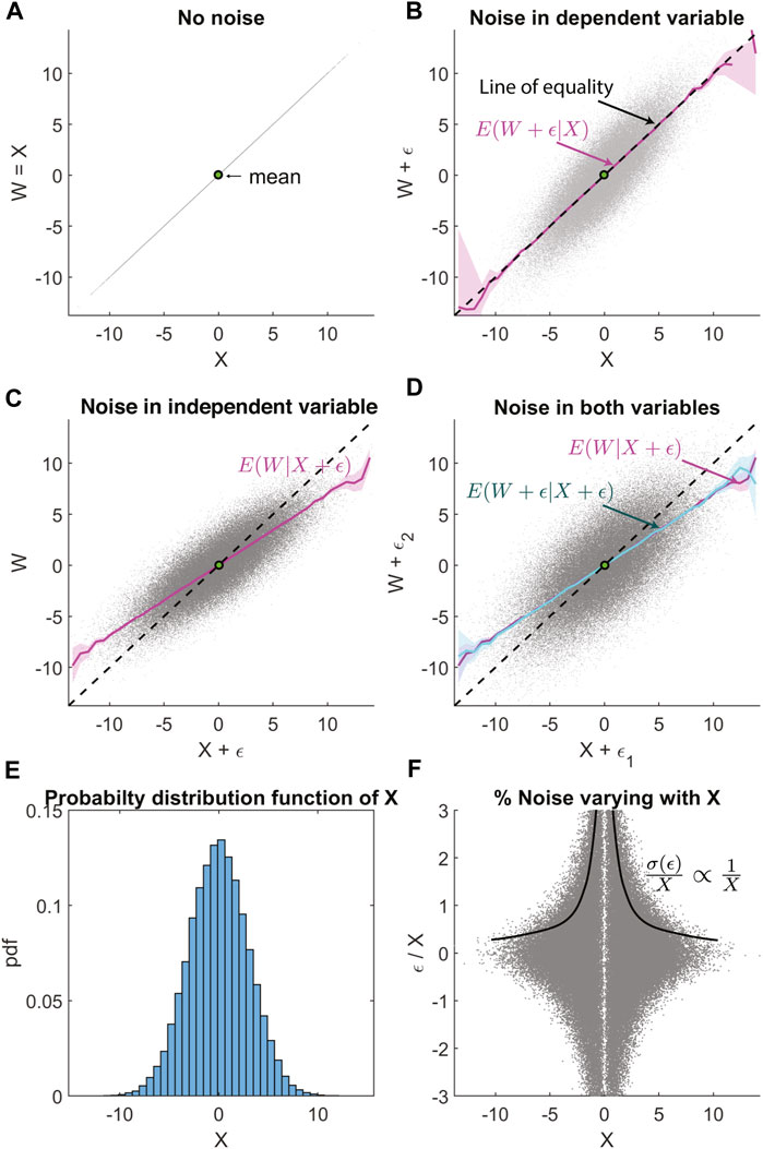
FIGURE 1. Regression bias in non-linear regression analysis between normally distributed random variables, with uncorrelated Gaussian noise. (A) Scatter plot of W vs. X, where X is a normally distributed random variable and W = X. (B) Uncorrelated Gaussian noise ϵ is added to W. Magenta line shows the conditional expectation E(W + ϵ|X). The dashed black line is the line of equality. (C) Uncorrelated Gaussian noise added only to X, with the magenta line E(W|X + ϵ) showing regression bias. (D) Uncorrelated Gaussian noise is added to both W and X, with regression bias in E(W + ϵ|X + ϵ) is visible in the cyan line. This overlaps with the magenta line that shows E(W|X + ϵ) for comparison. (E) Probability distribution function X showing the normal distribution with zero mean and standard deviation 3. (F) The fractional error ϵ/X that is varying inversely with X, as σ(ϵ) = constant.
However, when the relationship between the two variables is unknown, it is common to rely on regression analysis to infer their relationship. Regression analysis is a broad category of techniques used to find an association between two or more variables. Linear regression is the most familiar type of regression analysis, especially the method of ordinary linear least-squares that minimizes the sum of squared differences between the data points and a unique line on the plot. Suppose the relationship between W and X is linear. In that case, the best predictor of W given X is a line βX + c where the slope β and the intercept c are chosen to minimize the mean squared error between the vertical distance of the data and line from the x-axis. If we do not assume the relationship between W and X to be linear, then the function that minimizes the mean squared error between the vertical distance of itself and the data is
An approximate and common method of calculating the conditional expectation E(W|X) is to bin the data along the “independent” variable X and average the values of the “dependent” variable W within each bin. In this article, we use this method to estimate the conditional expectation, which we also refer to as the regression function or regression curve. This method of plotting the conditional expectation is used regularly in space physics. It is, in some instances, quite similar to the running average used by Borovsky (2021b), taken along the vertical axis for data sorted according to the magnitude of the parameter on the horizontal axis. Unlike the method of fitting functions, which gives equal weight to all data points, thereby restricting the fit to be dominated by the range of parameters with most points, calculating the conditional expectation through binning gives equal weight to every bin, and hence the non-linear function derived from it applies to the full range.
True values of W and X are always unavailable since we inevitably have some uncertainty ϵ in the measurements of these random variables. The source of this uncertainty can be instrumental error, our assumptions about what X or W actually measures, and uncertainty in the temporal association of the two parameters.
In Figure 1B, we add uncertainty ϵ in the dependent variable W. ϵ is also normally distributed with mean 0 and standard deviation 2. We used the Marsaglia and Tsang (1984) method to generate the random numbers. The data points now have a vertical spread about the line of equality as expected. And the non-linear regression function E(W|X) is also along the line of equality, giving us back the true relationship between W and X as the noise in W is averaged away.
In Figure 1C, we keep W free of uncertainty while including the same uncertainty ϵ in the independent variable X. Now, the regression function E(W|X) has a slope biased to a lower value. The conditional expectation coincides with the linear least-squares fit, and it happens because W and X + ϵ are jointly normally distributed. This bias is referred to as regression dilution bias for linear regression. This article uses the term regression bias and it includes biases caused even in non-linear regression, unlike “regression dilution bias” which is commonly used to describe biases observed for linear least-squares regression. The regression bias is a result of the “regression to the mean” effect. We explain these two important phrases found in statistics literature as follows.
1. Regression Dilution Bias: If the relationship between W and X is linear W = βX + c, and we only have access to the error-prone measurement X∗ = X + ϵ, then W = β(X∗ − ϵ) + c. Hence, the minimum mean squared estimate of the slope for the best linear prediction is
It follows that,
. Where λ is known as the attenuation factor, and 0 < λ < 1 because
2. Regression to the mean: A more fundamental explanation of the regression bias is the fact that measured extreme values are more likely to be values that are closer to the mean but are mistaken to be extreme due to uncertainty or measurement error (Barnett et al., 2005). In Figure 2, we show the probability density function of X—the true value we are attempting to measure. When a specific value of X occurs, our attempt to measure it with some uncertainty ϵ is shown with the conditional probability density function pdf(X*|X = 2) and pdf(X*|X = 4). These conditional probability density functions (in blue and red) show the probability that the true values X = 2 or X = 4, when measured, will appear as any other value X* on the real-line due to measurement error ϵ. When we measure X* = 3, the true value could be either X = 3 or any other value on the real line. However, the points where the conditional probability density functions intersect the vertical line X* = 3 show that it is more probable for X* = 3 to be actually X = 2 than X = 3 or X = 4. In fact, it is less probable that the true value of the measurement X* = 3 is X = 4 than X = 3 or X = 2. This is because it is much more likely for the mean value of a stochastic process to occur than an extreme value. The exact manner in which these biases happen depends on the nature of the measurement errors, the regression model, and the nature of the random variable or stochastic process.
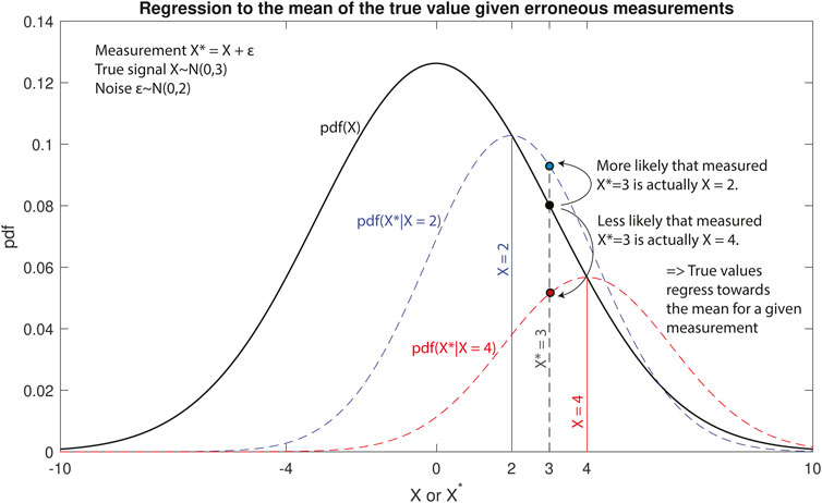
FIGURE 2. Demonstrating regression to the mean of the true value of an erroneous measurement. The black line is the underlying probability distribution of a random variable X. An erroneous measurement of X is X* = X + ϵ, where ϵ is uncorrelated Gaussian noise. One such measurement, X* = 3, is represented using the black dashed line. The likelihood that the true value X is also 3 is represented by the black filled circle on pdf(X). The blue dashed line is the conditional probability density function pdf(X*|X = 2), and it intersects line X* = 3 at the blue-filled circle, which represents the likelihood that the true value X is 2. Similarly, the red dashed line is the
The regression bias, quantified by the attenuation factor in the linear least-squares regression, is unaffected by uncertainty in the dependent variable W. This was seen in Figure 1B as E(W + ϵ|X) is unbiased. As a result, in Figure 1D, when we add uncertainty in both the dependent variable W and the independent variable X, the bias in the regression function E(W + ϵ|X + ϵ) remains the same as that observed in Figure 1C. An interesting consequence of this is that the reverse regression function E(X + ϵ|W + ϵ) will also have the same bias as E(W + ϵ|X + ϵ). If we interpret these regression functions without accounting for the regression bias, they appear to result in contradictory inferences. E(W + ϵ|X + ϵ) will imply that, on average, for extreme values, W* is an underestimate of X*, while E(X + ϵ|W + ϵ) implies the opposite, that on average X* is an underestimate of W*. This contradiction is an indicator of the existence of regression bias and that the nature of uncertainty in both variables is similar.
Figure 1E shows that the probability distribution function of X is a Gaussian, and Figure 1F shows how the percentage of uncorrelated Gaussian noise ϵ with respect to X varies with X. In this case, the noise fraction varies inversely with X (σ(ϵ|X = x)/X ∝ 1/X), since σ(ϵ|X = x) = constant. This depiction of the nature of measurement uncertainty will be useful as we demonstrate how the regression bias is affected by the uncertainty that is correlated with X below.
When X is not normally distributed but instead is log-normally distributed (Figures 3A,B,E), then the non-linear regression bias is no longer linear (Figures 3C,D). The log-normally distributed random number is generated by the transformation of a normally distributed random number generated by the Marsaglia and Tsang (1984) method. Here we have ensured that the error ϵ is still a zero-mean Gaussian with a standard deviation of 2, and it is uncorrelated with X or W (Figure 3F). The non-linearity is substantial, close to the mean value shown by the green dot, and the slope bends away from the line of equality towards the mean.
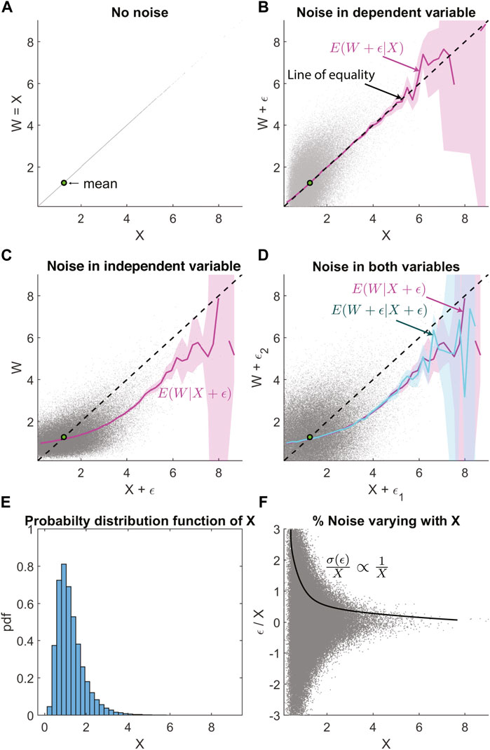
FIGURE 3. Similar layout as Figure 1, but with log-normal distribution and uncorrelated noise. (A) Scatter plot of W vs. X, where X is a log-normally distributed random variable and W = X. (B) Uncorrelated Gaussian noise ϵ is added to W. Magenta line shows the conditional expectation E(W + ϵ|X). The dashed black line is the line of equality. (C) Uncorrelated Gaussian noise added only to X, with the magenta line E(W|X + ϵ) showing regression bias. (D) Uncorrelated Gaussian noise is added to both W and X, with regression bias in E(W + ϵ|X + ϵ) is visible in the cyan line. This overlaps with the magenta line that shows E(W|X + ϵ) for comparison. (E) Probability distribution function X showing the log-normal distribution. (F) The fractional error σ(ϵ)/X that is varying inversely with X, as σ(ϵ) = constant.
When X is log-normally distributed (Figures 4A,B,E), and the error ϵ is correlated with X (Figure 4F) then the non-linear regression bias is even more non-linear, especially at extreme values (Figures 4C,D). The layout of Figure 4 is the same as Figure 1. The uncertainty ϵ is made to be proportional to |X|2; hence the noise fraction shown in Figure 4F increases linearly with X. This leads to a substantial non-linear bias in the non-linear regression function at values far away from the mean. The slope is biased away from the line of equality towards the mean value shown by the green dot. If we did not realize this as regression bias, then it is possible to misinterpret that E(W|X*) saturates with increasing X* and misattribute it to a physical cause or systematic instrument bias.
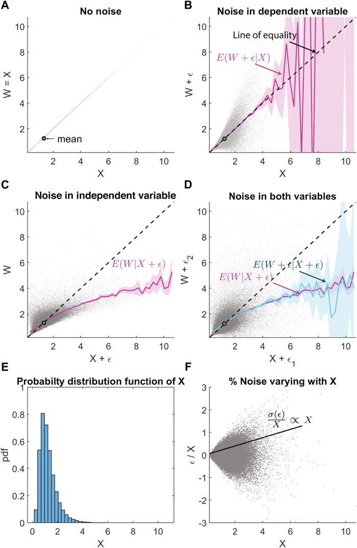
FIGURE 4. Similar layout as Figure 1, but with log-normal distribution and correlated noise such that σ(ϵ) ∝ X2. (A) Scatter plot of W vs. X, where X is a log-normally distributed random variable and W = X. (B) Correlated Gaussian noise ϵ is added to W. Magenta line shows the conditional expectation E(W + ϵ|X). The dashed black line is the line of equality. (C) Correlated Gaussian noise added only to X, with the magenta line E(W|X + ϵ) showing regression bias. (D) Correlated Gaussian noise is added to both W and X, with regression bias in E(W + ϵ|X + ϵ) is visible in the cyan line. This overlaps with the magenta line that shows E(W|X + ϵ) for comparison. (E) Probability distribution function X showing the log-normal distribution. (F) The fractional error is proportional to X.
By definition, the log-normal distribution X can be transformed to another random variable Z = log X which is normally distributed. Hence, if we know that the independent and dependent variables are jointly log-normally distributed, we can, in principle, take its logarithm and carry out a linear least-squares regression. For example one can estimate the coefficients of the linear regression function log W = β log X + c and then transform them back to the W vs. X coordinate system. The procedure was carried out by King and Papitashvili (2005) for solar wind density and temperature as they are log-normally distributed to estimate systematic biases between ACE and WIND measurements. However, as shown in Figures 5A–D, this log-linear least-squares fit (blue-line) also tracks the non-linear regression function (magenta line) reasonably well for all combination of uncertainties in W and X. This implies that the log-linear least-squares fit is susceptible to regression bias created by the log-normality of the independent variable and uncertainty in its measurements. Hence using the log-linear least-squares approach may result in misattributing regression bias to systematic biases between the space monitors.
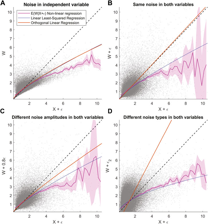
FIGURE 5. Comparing the effect of regression to the mean on non-linear regression, linear least-squares regression, and orthogonal regression function. Similar to Figure 4, X is log-normally distributed with W = X, and ϵ is Gaussian uncertainty that is correlated with X such that σ(ϵ) ∝ X2. (A) Shows different regression fits on data with uncertainty added only to X. (B) Shows the same with added uncertainty and the same characteristics on both X and W. (C) Shows the same but with slightly less uncertainty added to W compared to X. (D) Shows the same plot with uncorrelated Gaussian uncertainty ϵ2 added to W, while correlated Gaussian uncertainty ϵ as in B is added to X.
A relatively popular method considered to be capable of avoiding regression bias is the orthogonal regression function. The orange line in Figures 5A–D is the orthogonal linear regression fit for the corresponding data set. And it retrieves the true relationship between X and W in the case where the same error ϵ is present in both variables. This is because orthogonal linear regression minimizes the sum of the squared orthogonal distances between all (W, X) points and a unique line, and it has an unbiased slope only when the uncertainty in both variables is equal. A more general orthogonal regression method (total least squares regression) includes the information on the ratio of uncertainties in both W and X and can correct the regression bias much more effectively. In general, to correct the regression bias, we need to possess a quantitative knowledge of the uncertainty in X and W—not just the probability distribution of ϵ but also the conditional probability distribution pdf(ϵ|X) (e.g., Morley et al., 2018).
Uncertainties are commonly characterized by referring to the standard deviation or variance of X∗ − ⟨X∗⟩ = ϵ. However, the severity of the regression bias cannot be judged solely on a parameter like the standard deviation or variance of the noise ϵ. It is affected by the nature of the correlation of ϵ with X and even other variables that may, in turn, affect X. Figure 6 provides a demonstration of this argument. The top and bottom panels show regression bias in the non-linear regression of W vs. X + ϵ, where W and X have the same log-normal distributions. The only difference between the top and bottom panels is the uncertainty in the independent variable X, which is a function of ϵ1(X) ∝ X2 for the top while ϵ2(X) = constant for the bottom panel. Therefore the noise fraction ϵ1/X ∝ X and ϵ2/X ∝ 1/X as seen in Figures 6B,E respectively. The rightmost column (Figures 6C,F) shows plots of the marginal distribution of the noise ϵ1 and ϵ2 i.e., pdf(ϵ1) and pdf(ϵ2). Here the common metric used to quantify unbiased noise, the standard deviation, has the value of 0.5 for ϵ1 and 1 for ϵ2. Since σ(ϵ1) < σ(ϵ2) one may assume that there is less noise in X for the top panel than the bottom, and hence less regression bias. This is true close to the mean; however, further away from the mean, the regression bias is more severe for panel 1 (Figure 6A) than panel 2 (Figure 6D) as ϵ1 is correlated with X while ϵ2 is not.
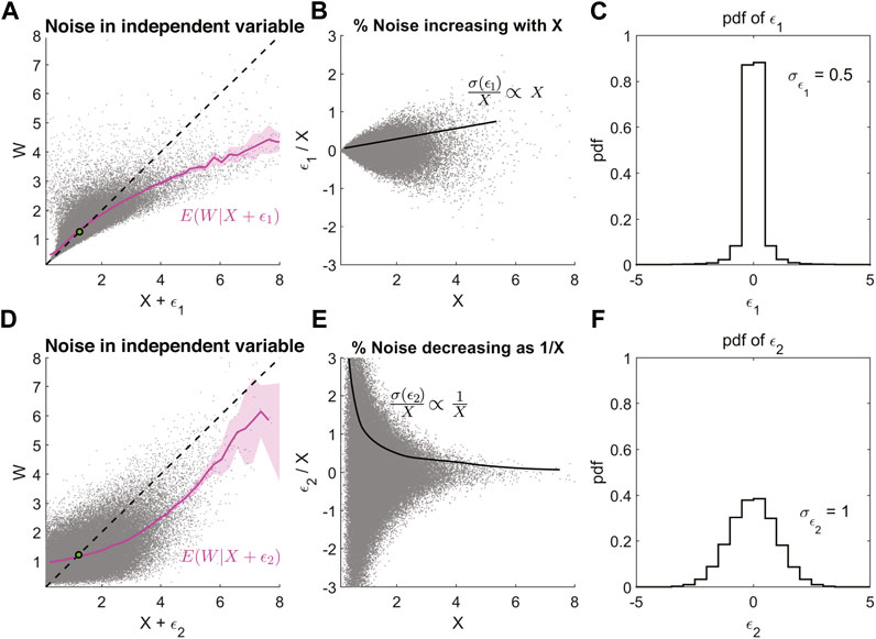
FIGURE 6. The severity of the regression bias at extremes is not determined only by the standard deviation of the uncertainty ϵ. It is also necessary to know how the noise is correlated with the independent variable. (A) Magenta line is the E(W|X + ϵ1) where ϵ1 is correlated Gaussian noise. (B) Fractional error or noise ϵ1/X increasing linearly with X, since σ(ϵ1) ∝ X2. (C) The marginal probability distribution of ϵ1, with the standard deviation of ϵ1 = 0.5. (D) Same as (A) but with uncorrelated Gaussian noise ϵ2 added to X. (E) Fractional error or noise ϵ2/X decreasing as 1/X, since σ(ϵ2) = constant. (F) The marginal probability distribution of ϵ2, with the standard deviation of ϵ2 = 1.
3 Comparing Solar Wind Monitors
The previous section demonstrates that uncertainty in the independent variable can lead to a bias in the regression function. Such biases are unavoidable whether we use non-linear regression, linear least-squares regression, or orthogonal linear regression. However, we can correct the bias with a quantitative knowledge of the uncertainties, its direct or indirect correlation with the independent variable, and the probability distribution underlying the independent variable. In this section, we show regression biases in comparisons between solar wind monitors and suggest that at least part of these results are from random uncertainty in solar wind measurements rather than systematic instrument biases.
The solar wind monitors we use are the ACE and WIND satellites. They mostly measure solar wind plasma and magnetic fields upstream of the Earth’s magnetospheric bow shock. We use 1-min spacecraft-specific data compiled by the OMNI database, which are time-shifted using a propagation model to the bow shock. Following is a look at non-linear regression between ACE and WIND measurements of multiple solar wind parameters. They should lie along the line of equality if both spacecraft measure the same solar wind plasma and magnetic field on average without uncertainty. However, that is not the case. Substantial regression biases towards the mean of the parameter can be observed for extreme values, especially when the monitors are far apart.
3.1 Solar Wind Velocity Vy and Vz
Figures 7A,B show scatter plots of time-shifted solar wind velocity components along the Z-GSE direction measured simultaneously by ACE and WIND spacecraft over 20 years. The black dashed line is the line of equality with a 45° slope, along which we would expect an unbiased ACE and WIND measurement to lie. However, a non-linear regression of ACE Vz GSE measurements given WIND Vz GSE and vice versa, shown by the magenta line, has a slope reduced towards the mean. The regression curve in Figures 7A, B seem to suggest a contradiction. The former suggests that ACE underestimates Vz GSE on average compared to WIND for extreme values. However, the latter suggests that WIND underestimates Vz GSE on average compared to ACE. We can explain the contradiction if we suppose that the biases of these regression curves come from similar uncertainty in both ACE and WIND measurements, as discussed concerning Figure 1D in the previous section. And since systematic measurement bias cannot lead to contradictory regression curves, the regression bias in Figure 7 cannot possibly arise from systematic biases in the ACE and WIND measurements. However, we cannot rule out the existence of systematic measurement bias without a more careful analysis of quantifying random uncertainties. Figures 7C,D shows similar regression bias in ACE and WIND measurements of Vy GSE. At large values of ACE Vy ∼ 200 km/s, on average WIND measures a
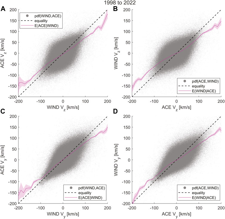
FIGURE 7. Regression bias in solar wind velocity Vz and Vy in GSE coordinates. (A) Shows a scatter plot of 1-min resolution propagation delay-corrected ACE Vz vs. WIND Vz. The dashed black line is the line of equality, and the magenta line is the conditional expectation
3.2 Solar Wind IMF Bz
The primary cause of this non-trivial regression bias is the uncertainty stemming from the spatial and temporal separation of the measurements. As a result, both spacecraft do not see the same solar wind magnetic field or plasma most of the time. A useful measure of whether a downstream spacecraft measures the same plasma element previously seen by an upstream spacecraft is the impact parameter (IP). For WIND and ACE, the impact parameter (IP) is the “minimum distance experienced between WIND moving at 30 km/s in Y and plasma element moving at 390 km/s in X” (King and Papitashvili, 2005; Papitashvili, 2005).
Figures 8A,C plots ACE vs. WIND measurements of Bz GSM and vice-versa for all data points in the year 2002. In 2002, WIND was not yet parked onto its L1 orbit, and as a result, the IP between ACE and WIND is significant for most measurements. Figures 8B,D plot the regression between ACE and WIND Bz and vice versa for IP less than 60 RE, implying that they both likely see similar solar wind plasma. An IP of less than 60RE is considered to be the minimum separation for which WIND and ACE will see similar plasma and magnetic fields (King and Papitashvili, 2005). In this case, the regression bias is substantially reduced, as the regression curves almost align with the line of equality. This indicates that regression biases can exacerbate while using ACE and WIND data when they are far away from each other (IP
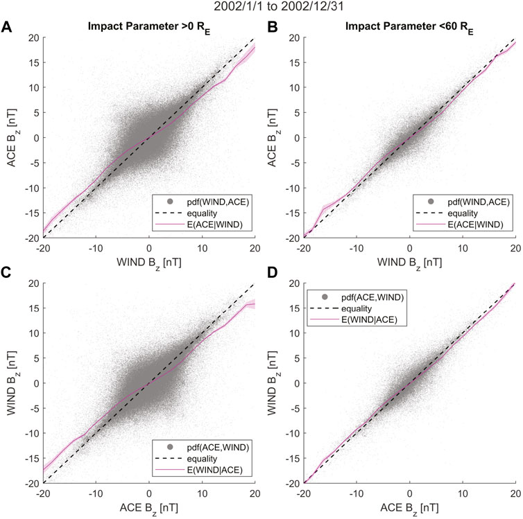
FIGURE 8. Regression bias in solar wind magnetic field Z-GSM component. The bias reduces when filtering the data used by reducing the impact parameter (IP) between ACE and WIND. (A) Shows a scatter plot of simultaneous 1-min resolution propagation delay-corrected ACE Bz vs. WIND Bz. The measurements used were from the year 2002. The dashed black line is the line of equality, and the magenta line is the conditional expectation
3.3 Solar Wind Proton Number Density N
Figure 9 shows the solar wind proton number density comparison between ACE and WIND measured during two time periods: column 1–1998 to 2001 pre solar maximum and column 2–2002 to 2005 post solar maximum. The dotted black line is the line of equality, while the magenta line is the non-linear regression function, and the blue line is the same but only includes measurements with ACE-WIND IP less than 60 RE. The first panel shows the regression function of ACE given WIND measurements, while the second panel plots the reverse: WIND given ACE measurements. We see that there is a regression bias with a decreasing slope with increasing density for Figures 9A–D. The bias is more severe further away from the mean of the density measurements. From the density of the scatter plots, we can see that there are fewer proton number density measurements overall in the years 2002–2005 as compared to 1998 to 2001. Indicating that the underlying probability distribution of the proton number density can indeed change with the solar cycle, and regression bias can be time-dependent. Reducing the IP does not seem to change the regression function much, except for Figure 9D, where it has a substantial effect on making the regression function align with the line of equality. This could suggest that even the random uncertainty in measuring the solar wind parameters may change depending on the periods of the measurements, as the spacecraft’s relative location also vary with time.
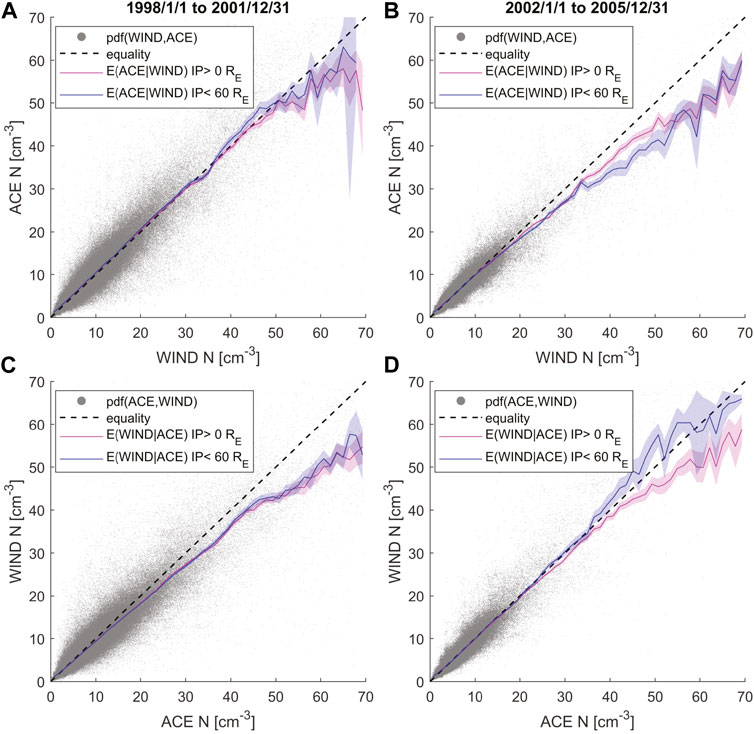
FIGURE 9. Regression bias in solar wind proton density. It reduces when filtering the data to IP
For the regression functions shown here, the non-linear decrease in the slope with increasing density is due to the log-normal distribution of density, similar to the numerical experiment described in Figure 4. According to King and Papitashvili (2005) ACE proton number densities are systematically larger than WIND number densities by up to 18% for higher solar wind speeds. They carried out a log-linear least squares regression, only for WIND vs. ACE and not the reverse. The systematic bias they estimate for higher solar wind speeds suggests ACE overestimates the densities. Curiously this bias is in the same direction we’d expect if the systematic bias was regression bias instead. However, our analysis in this article does not quantitatively delineate the two biases, as it requires careful correction of the regression bias.
3.4 Solar Wind IMF Clock Angle θcl
The IMF clock angle is an essential solar wind parameter determining the extent of solar wind energy coupling to the magnetosphere. The rate of the day-side reconnection, in part, is influenced by the relative orientation of the solar wind magnetic field direction (modified by the magnetosheath). For example, in simple magnetic reconnection models, two oppositely directed magnetic fields brought together by moving plasma drive reconnection. Hence, a southward IMF can generally trigger day-side reconnection at the sub-solar point, while a northward IMF does not. As a result, many proposed solar wind driver functions, which estimate the energy coupling between the solar wind and the magnetosphere, are some functions of the IMF clock angle (Newell et al., 2007; Borovsky, 2008; Lockwood and McWilliams, 2021).
The IMF clock angle is defined as the angle between the IMF vector projected on the GSM Y-Z plane and the geomagnetic north: θcl = atan2(BY, BZ) where −180° < θcl < 180°. In this manuscript, we have constructed θcl to range from 0° to 360° with 0° pointing towards BZ north. In Figure 10A, we compare 1 min-resolution measurement of the ratio BY/BZ of ACE vs. WIND and plot the conditional expectation of the ACE BY/BZ given WIND BY/BZ (magenta line). The blue line is the same non-linear regression function but with measurements where ACE and WIND have an impact parameter less than 60 RE. Figure 10C plots the reverse regression of WIND vs. ACE. Both plots show regression bias towards the mean for extreme values (for |By/Bz|∼ > 2). Large values of the BY/BZ ratio are mostly a result of small BZ values. The latter corresponds to
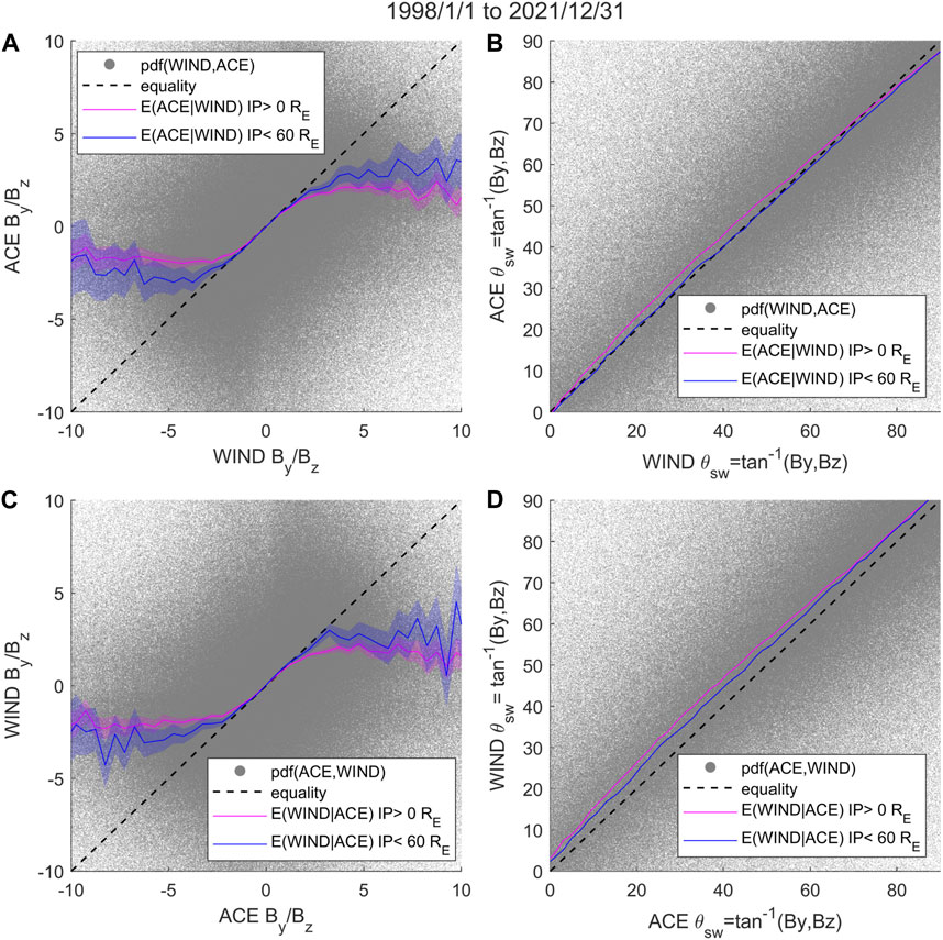
FIGURE 10. Regression bias in Solar Wind IMF Clock Angle. (A) Regression function
Figures 10B,D show the ACE vs. WIND regression curve of the IMF clock angle and its reverse, respectively. Though the measurements span 0°–360°, the plot only shows the clock angles 0°–90° to highlight the bias in the regression curve, which has a slope that increases from the line of equality and then decreases. The regression bias reduces when the impact parameter is limited to less than 60 RE in both plots. The conditional expectation is calculated using directional statistics, as an arithmetic mean is inappropriate for angles. Here the mean is calculated by first converting the IMF clock angle into a complex number through Euler’s formula to consider how angles wrap around 360°. Then the arithmetic mean is calculated of the resulting complex numbers. This value is then converted back to an angle to obtain the conditional expectation.
To explore the nature of the bias in detail, Figure 11 plots the regression bias in polar coordinates. Figure 11A shows the probability density function of the IMF clock angle as measured by ACE from 1998 to 2022 along the radial axis. The polar angle coordinates represent
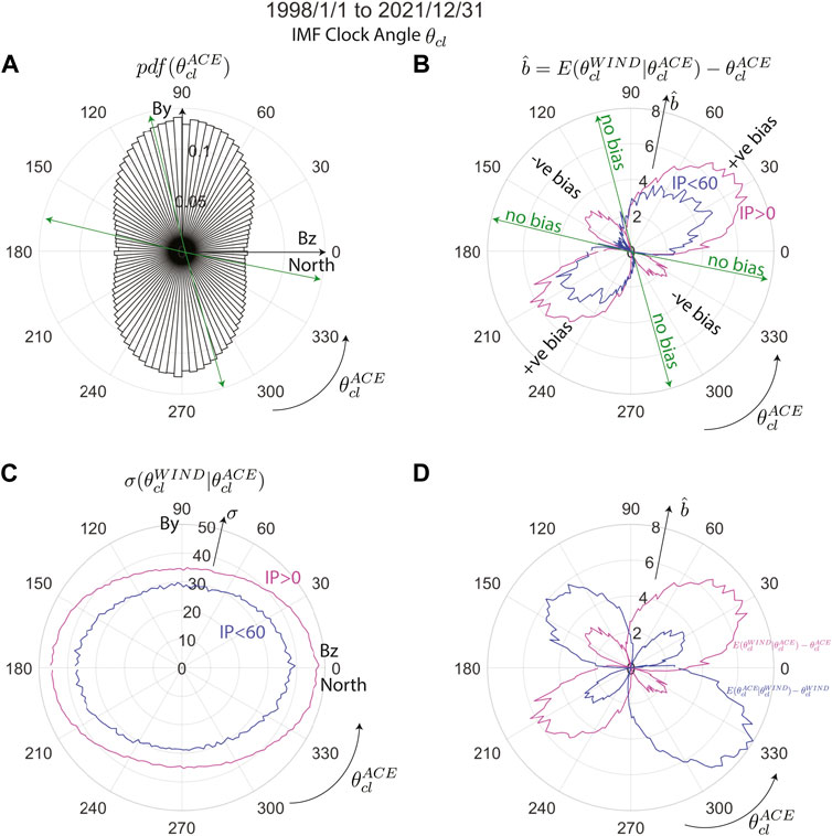
FIGURE 11. Polar plots of regression bias in solar wind IMF clock angle. (A) Circular probability density function of IMF clock angle, defined as
The regression bias is at a highest of ∼ + 7° around
Close to the local pdf minimum
Figure 11D plots the bias in the IMF clock angle regression curve of ACE vs. WIND (magenta line) and its reverse (blue line). The same cycle of positive and negative bias as Figure 11B is seen for both the regression curves. However the positive bias is lesser and negative bias is greater for
Figure 11C shows the standard deviation of WIND measurements of the IMF clock angle given ACE measurements of the same (shown in the magenta curve). The maximum uncertainty in the IMF clock angle measurements occurs when ACE measures northward and southward IMF Bz (
3.5 Solar Wind Driver Function Esw
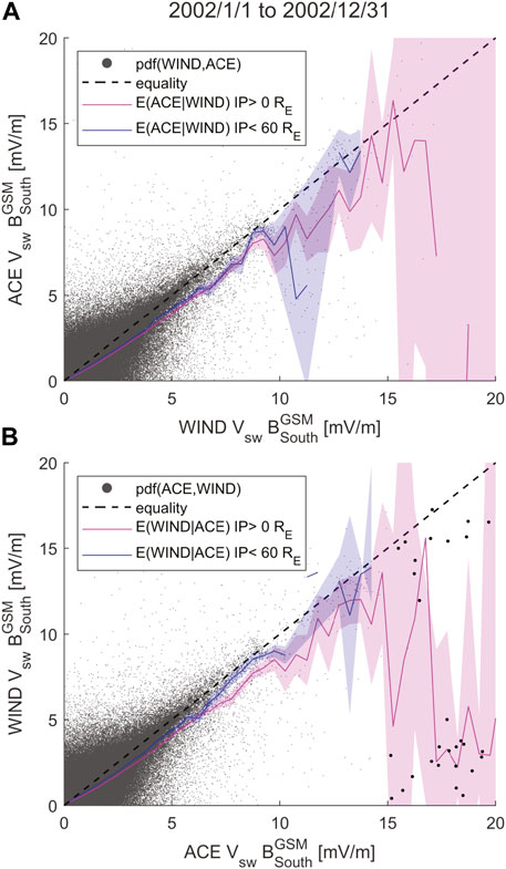
FIGURE 12. Regression bias in solar wind driver function Esw = VswBsouth, where
For example, consider the data points highlighted using larger dots in Figure 12B. Here ACE measures Esw values between 15 and 20 mV/m and WIND measures some of it to be much lower - between
4 Discussion
Results in section 3 show that regression bias exists for important solar wind parameters like IMF Bz, clock angle θcl and solar wind proton number density N. Many other parameters also exhibit such regression biases, especially for extreme values of their measurements. Hence if we do not carefully account for random uncertainties in the solar wind parameters, any effort to identify instrument biases by comparing data sets may misinterpret regression bias as systematic instrument bias.
Uncertainties in complex parameters such as solar wind driver functions, which are a combination of solar wind parameters, may be correlated with the parameter’s value. Consider the example of the merging electric field: Em = VBT sin2θcl/2. An uncertainty Δθ in θcl, will result in an erroneous merging electric field
Therefore, the uncertainty in the merging electric field:
Many solar wind driver functions are empirically constructed formulas and are not necessarily derived from physical principles. Hence true solar wind driver functions may be biased or different in a random sense or both. It is easy to imagine that the estimate of the solar wind drivers using upstream solar wind monitors differs randomly from the platonic “true” driver function that affects the Earth’s response. Suppose the driver function is in the form of the merging electric field. In that case, random uncertainty in one of the parameters can lead to correlated uncertainties in the merging electric field. However, if, instead, they are in the form of a sum of parameters like Vsw + 56Bz (Borovsky, 2014), then the uncertainties will not be correlated with the magnitude of the driver. Hence, one may expect less regression bias. This could be the reason why the above unphysical solar wind driver formula has better correlations with geomagnetic activity than all other standard solar-wind functions (Newell et al., 2007; Borovsky, 2008; Borovsky, 2021a). Hence, the uncertainty in the solar wind driver functions and the regression bias it causes may be contributing to the math-versus-physics dilemma discussed by Borovsky (2021a). Once we account for the uncertainties, the physics-based formula may be more correlated than the other unphysical math-based ones.
Random uncertainties in the solar wind drivers are not just limited to spatial and temporal uncertainty in the solar wind measurements and instrumental errors (Lockwood, 2022). (Though these are likely the primary source of uncertainties in ACE and WIND measurements used in this manuscript.) Another important source of error is the effect of bow shock and magnetosheath on the solar wind IMF at the day-side. For example, Coleman (2005) shows a
Borovsky (2022) proposes that the functional form of the solar wind drivers ought to be constructed taking into account the uncertainties and the regression bias it creates. We believe this is crucial, as otherwise, regression bias in regression analysis of the driver functions and earth’s response may be misinterpreted as caused by physical processes rather than uncertainty. Machine-learning-based models that use non-parametric non-linear regression analysis may also be susceptible to such biases. With the recent proliferation of many such models in space physics, we believe these biases are important to consider. A plausible example of regression bias, either partially or wholly misunderstood as caused by physical processes, could be the saturation of the polar cap potential and other geomagnetic indices (Borovsky, 2021b).
The “regression towards the mean effect” may not only be relevant to statistical regression analysis. It affects individual studies of extreme solar wind driving and the Earth’s response to it. The reason for this is that the regression bias affects the entire conditional probability distribution of the measurements being compared. Hence, when we infer the Earth’s response to an extreme solar wind driving, it is likely that the actual value of the solar wind driver is lower and closer to its mean value. Hence, we may be underestimating the effect of the solar wind driving of geomagnetic activity even for a single event or case study.
A more precise way to describe the “regression towards the mean effect” is perhaps apparent in Figure 11. Here the distribution is bi-modal and has two regions of high probability in the parameter space (
The natural question from our analysis is what we can do to correct or mitigate regression bias. Two primary directions here are 1) to quantify the uncertainty and calibrate the data to compensate for the bias, or 2) to improve the quality of the data by reducing uncertainty. For the case of ordinary linear least-squares regression, orthogonal regression that considers uncertainty in both dependent and independent variables can correct the bias. However, for non-linear regression, these methods may be insufficient. Therefore a careful analysis of correlated uncertainties and stochastic properties of the measured parameters are necessary to construct error models that estimate the regression bias. After this, one can apply the technique of regression calibration to the uncertain measurements and calculate the likely true values to correct for the bias in the inferred relationship. Many more techniques exist and are discussed extensively in Carroll et al. (2006).
The main challenge to constructing error models to carry out regression calibration is quantifying the uncertainties in the measurement parameters. In most cases, the uncertainties involved are not just instrumental errors but uncertainties that stem from the implicit assumptions made in interpreting measurements. For example, in the case of the solar wind driver functions—random uncertainties stem from our assumptions of: 1) solar wind propagation models, 2) solar wind structure, 3) solar wind interaction with bow-shock and magnetosheath plasma, 4) valid solar wind and magnetosphere state parameters. More assumptions may exist, but the first step towards quantifying random uncertainty in solar wind parameters (including driver functions) is to identify the assumptions and then estimate their contribution to the uncertainty through physics or mathematical models.
5 Summary
We used simple numerical experiments to demonstrate the statistical phenomenon of regression towards the mean, which leads to biases in the correlation between measurement parameters. We showed evidence for such biases while comparing simultaneous 1-min resolved propagation delay-corrected ACE and WIND measurements of several solar wind parameters upstream of the magnetosphere bow-shock. The regression biases were significant for extreme values of the measurement parameters. For example when WIND measures
These results suggest that regression biases may exist in statistical and event-based solar-wind/magnetosphere coupling studies, where the magnetosphere’s response to solar wind driving is inferred from measurements. The bias may become significant for rare and extreme driving conditions and if the uncertainties in the driver functions correlate with the solar wind strengths. We can reliably correct the regression bias only by knowing the stochastic properties of the parameters used in the study and their uncertainties. Not accounting for the effect of these uncertainties may lead to misinterpreting the bias (which can sometimes be non-linear) as systematic measurement bias or physical processes. One such possible misinterpretation could be the saturation of geomagnetic indices observed with increasing solar wind driving (Borovsky, 2021b).
Data Availability Statement
The datasets analyzed for this study, and the corresponding MATLAB code used to visualize the plots in this article can be found in the repository https://doi.org/10.5281/zenodo.6604150. For non-MATLAB users, the code and its output is accessible as HTML files in the repository. All data we have used is publicly available. We thank GSFC/SPDF OMNIWeb service for the spacecraft specific 1 min resolution data sets of WIND and ACE measurements propagated to the bow shock. This can be accessed from https://spdf.gsfc.nasa.gov/pub/data/omni/high_res_omni/sc_specific/.
Author Contributions
NS conceptualized this project, performed the analysis, and wrote the manuscript. DS supervised and conceptualized the work, and reviewed the manuscript.
Funding
NASA Cooperative Agreement 80NSSC21M0180G: Partnership for Heliophysics and Space Environment Research (NS) NASA Heliophysics Participating Investigator Program under Grant WBS516741.01.24.01.03 (DS).
Conflict of Interest
The authors declare that the research was conducted in the absence of any commercial or financial relationships that could be construed as a potential conflict of interest.
Publisher’s Note
All claims expressed in this article are solely those of the authors and do not necessarily represent those of their affiliated organizations, or those of the publisher, the editors and the reviewers. Any product that may be evaluated in this article, or claim that may be made by its manufacturer, is not guaranteed or endorsed by the publisher.
Acknowledgments
We thank Bob Robinson at the Catholic University of America for discussions and support. We also wish to acknowledge Joe Borovsky, Maria-Theresia Walach, Varsha Subramanyan, Dogacan Ozturk, Banafsheh Ferdousi, Gonzalo Cucho-Padin and Abigail R. Azari for valuable discussions.
Supplementary Material
The Supplementary Material for this article can be found online at: https://www.frontiersin.org/articles/10.3389/fspas.2022.924976/full#supplementary-material
References
Barnett, A. G., van der Pols, J. C., and Dobson, A. J. (2005). Regression to the Mean: What it is and How to Deal with it. Int. J. Epidemiol. 34, 215–220. doi:10.1093/IJE/DYH299
Borovsky, J. E. (2014). Canonical Correlation Analysis of the Combined Solar Wind and Geomagnetic Index Data Sets. J. Geophys. Res. Space Phys. 119, 5364–5381. doi:10.1002/2013JA019607
Borovsky, J. E. (2021a). Is Our Understanding of Solar-Wind/Magnetosphere Coupling Satisfactory? Front. Astron. Space Sci. 8, 5. doi:10.3389/FSPAS.2021.634073/BIBTEX
Borovsky, J. E. (2022). Noise, Regression Dilution Bias, and Solar-Wind/Magnetosphere Coupling Studies. Front. Astron. Space Sci. 9, 45. doi:10.3389/fspas.2022.867282
Borovsky, J. E. (2021b). On the Saturation (or not) of Geomagnetic Indices. Front. Astron. Space Sci. 8, 175. doi:10.3389/FSPAS.2021.740811/BIBTEX
Borovsky, J. E. (2008). The Rudiments of a Theory of Solar Wind/magnetosphere Coupling Derived from First Principles. J. Geophys. Res. 113, 8228. doi:10.1029/2007JA012646
Borovsky, J. E. (2018). The Spatial Structure of the Oncoming Solar Wind at Earth and the Shortcomings of a Solar-Wind Monitor at L1. J. Atmos. Sol.-Terr. Phys. 177, 2–11. doi:10.1016/j.jastp.2017.03.014
Camporeale, E. (2019). The Challenge of Machine Learning in Space Weather: Nowcasting and Forecasting. Space Weather 17, 1166–1207. doi:10.1029/2018SW002061
Carroll, R. J., Ruppert, D., Stefanski, L. A., and Crainiceanu, C. M. (2006). Measurement Error in Nonlinear Models: A Modern Perspective, Second Edition. Baco Raton: Chapman & Hall/CRC, 1–455.
Case, N. A., and Wild, J. A. (2012). A Statistical Comparison of Solar Wind Propagation Delays Derived from Multispacecraft Techniques. J. Geophys. Res. 117, 2101. doi:10.1029/2011JA016946
Coleman, I. J. (2005). A Multi-Spacecraft Survey of Magnetic Field Line Draping in the Dayside Magnetosheath. Ann. Geophys. 23, 885–900. doi:10.5194/ANGEO-23-885-2005
Frost, C., and Thompson, S. G. (2000). Correcting for Regression Dilution Bias: Comparison of Methods for a Single Predictor Variable. J. R. Stat. Soc. A 163, 173–189. doi:10.1111/1467-985x.00164
Fuller, W. A. (1987). Measurement Error Models. New York: John Wiley & Sons. doi:10.1002/9780470316665
King, J. H., and Papitashvili, N. E. (2005). Solar Wind Spatial Scales in and Comparisons of Hourly Wind and Ace Plasma and Magnetic Field Data. J. Geophys. Res. 110, 2104. doi:10.1029/2004JA010649
Lockwood, M., Bentley, S. N., Owens, M. J., Barnard, L. A., Scott, C. J., Watt, C. E., et al. (2019). The Development of a Space Climatology: 1. Solar Wind Magnetosphere Coupling as a Function of Timescale and the Effect of Data Gaps. Space Weather 17, 133–156. doi:10.1029/2018sw001856
Lockwood, M., and McWilliams, K. A. (2021). On Optimum Solar Wind‐Magnetosphere Coupling Functions for Transpolar Voltage and Planetary Geomagnetic Activity. JGR Space Phys. 126, e2021JA029946. doi:10.1029/2021JA029946
Lockwood, M., Rouillard, A. P., Finch, I., and Stamper, R. (2006). Comment on "The IDV Index: Its Derivation and Use in Inferring Long-Term Variations of the Interplanetary Magnetic Field Strength" by Leif Svalgaard and Edward W. Cliver. J. Geophys. Res. 111, A09109. doi:10.1029/2006JA011640
Lockwood, M. (2022). Solar Wind-Magnetosphere Coupling Functions: Pitfalls, Limitations, and Applications. Space Weather 20, e2021SW002989. doi:10.1029/2021SW002989
Marsaglia, G., and Tsang, W. W. (1984). A Fast, Easily Implemented Method for Sampling from Decreasing or Symmetric Unimodal Density Functions. SIAM J. Sci. Stat. Comput. 5, 349–359. doi:10.1137/0905026
McPherron, R. L., Baker, D. N., Pulkkinen, T. I., Hsu, T.-S., Kissinger, J., and Chu, X. (2013). Changes in Solar Wind-Magnetosphere Coupling with Solar Cycle, Season, and Time Relative to Stream Interfaces. J. Atmos. Sol.-Terr. Phys. 99, 1–13. doi:10.1016/j.jastp.2012.09.003
Morley, S. K., Welling, D. T., and Woodroffe, J. R. (2018). Perturbed Input Ensemble Modeling with the Space Weather Modeling Framework. Space Weather 16, 1330–1347. doi:10.1029/2018sw002000
Newell, P. T., Sotirelis, T., Liou, K., Meng, C.-I., and Rich, F. J. (2007). A Nearly Universal Solar Wind-Magnetosphere Coupling Function Inferred from 10 Magnetospheric State Variables. J. Geophys. Res. 112, 1206. doi:10.1029/2006JA012015
Taylor, J. R. J. R. (1982). An Introduction to Error Analysis: The Study of Uncertainties in Physical Measurements. Sausalito, California: University Science Books.
Keywords: uncertainty, regression to the mean, solar wind magnetosphere coupling, space weather, regression dilution bias, noise
Citation: Sivadas N and Sibeck DG (2022) Regression Bias in Using Solar Wind Measurements. Front. Astron. Space Sci. 9:924976. doi: 10.3389/fspas.2022.924976
Received: 21 April 2022; Accepted: 01 June 2022;
Published: 04 July 2022.
Edited by:
Joseph E. Borovsky, Space Science Institute, United StatesReviewed by:
Brian Walsh, Boston University, United StatesMike Lockwood, University of Reading, United Kingdom
Copyright © 2022 Sivadas and Sibeck. This is an open-access article distributed under the terms of the Creative Commons Attribution License (CC BY). The use, distribution or reproduction in other forums is permitted, provided the original author(s) and the copyright owner(s) are credited and that the original publication in this journal is cited, in accordance with accepted academic practice. No use, distribution or reproduction is permitted which does not comply with these terms.
*Correspondence: Nithin Sivadas, c2l2YWRhc0BjdWEuZWR1
 Nithin Sivadas
 David G. Sibeck