A review of the theory of 3‐D Alfvén (field line) resonances

This review article aims to summarise recent developments in Alfvén resonance theory, with a focus on applications to magnetospheric ultra-low frequency (ULF) waves, though many of the ideas are relevant for applications in other fields as well. The key aspect we treat is how Alfvén resonance manifests in a fully 3-D varying medium. The prerequisite ideas are developed in a reasonably comprehensive introduction, which would be a good starting point for any interested reader looking to gain an understanding of the Alfvén resonance process, as well as where to find associated reading. The main part of the review is split into three sections. We firstly consider results from numerical simulations of relatively simple magnetic field geometries, such as 2-D and 3-D dipoles, to develop the fundamental properties of 3-D Alfvén resonances. Secondly, we review previous simulations in more general magnetic field geometries, reconciling these results with those from the simpler dipole cases. Thirdly, in light of these numerical results, we review theoretical studies using various analytical methods to find approximate solutions to the pertinent magnetohydrodynamic (MHD) equations. The review is concluded with a discussion of these different approaches, as well as linking these ideas to their importance for observations. Finally, we discuss potential future developments in this research area.

1 Introduction

Magnetohydrodynamic (MHD) wave processes operate throughout the heliosphere, from the solar corona to planetary magnetospheres. The MHD approximation requires the assumption of large length and time scales, which suits the description of, for example, low frequency plasma waves of a scale size on the order of the magnetosphere or a coronal loop. Indeed, MHD has been successfully used for decades to further our understanding of such oscillations. This review will predominantly be placed within the context of Earth’s magnetosphere, however, the MHD wave process elucidated will have applications further afield, to the other planetary magnetospheres and the low β solar corona. At Earth, the lowest frequency, largest scale plasma waves are called ultra-low frequency (ULF) waves. They have wide-ranging importance, from driving field-aligned currents which energise particles to precipitate into the upper atmosphere generating aurora (e.g. Milan et al., 2001; Rankin et al., 2005), to the interaction with energetic radiation belt particles causing acceleration, transport or loss (Elkington et al., 1999, 2003; Degeling et al., 2007; Zong et al., 2009; Claudepierre et al., 2013; Mann et al., 2013; Zong et al., 2017).

We focus on a particular MHD wave process known by many names depending on the field in which it is studied: fast-Alfvén wave coupling, Alfvén resonance, field line resonance and resonant absorption. All of these terms describe the transfer of energy from a global wave which can propagate across magnetic field lines, the MHD fast wave (henceforth simply called the fast wave/mode), to a local, strictly field-aligned wave, the MHD Alfvén wave (Alfvén, 1942). This energy transfer occurs when there is a frequency matching (i.e., resonance) between the two waves. At Earth, Dungey (1955) first made the connection between long period (a few minutes) magnetic field oscillations observed by ground magnetometers, and Alfvén waves standing along geomagnetic field lines. It was only later explained that the observed spatial variation and occurrence of these waves (Samson et al., 1971) could be attributed to the previously described wave-coupling process known at Earth as field line resonance (FLR) (Chen and Hasegawa, 1974; Southwood, 1974).

The most natural way to describe the development of FLR theory is to separate studies by the number of spatial dimensions in which the model equilibrium is inhomogeneous. At first, only a 1-D variation in the plasma equilibrium was considered, allowing the Alfvén speed to vary radially across a uniform, straight background magnetic field (Southwood, 1974; Kivelson and Southwood, 1986; Inhester, 1987). Known as the hydromagnetic box model, this is the simplest configuration to provide the required inhomogeneity to couple fast and Alfvén waves (in a uniform medium the waves are decoupled). The resulting Alfvén wave has a displacement/magnetic field perturbation in the azimuthal direction. By convention this is termed a toroidally polarised Alfvén wave, after the magnetic rather than electric field orientation.

In the 1-D regime, several important characteristics of FLR were established; properties which were later also proved to hold in 2-D. In the absence of dissipation (i.e., ideal MHD), assuming there exists a consistent fast wave to drive the resonance, the Alfvén wave amplitude will grow continuously in time. The spatial width of the resonance will also decrease to a delta function, as is typical of a driven harmonic oscillator without damping. Dissipation, in the form of finite ionospheric conductivity, limits the resonance amplitude, reaching the steady state where energy fed in to the resonance from the fast wave balances that dissipated through ohmic heating in the ionosphere (Southwood, 1974). At this point, the resonance will have a finite width, which depends upon the ratio of ionospheric and Alfvén conductances as well as the gradient of the Alfvén frequency (Southwood and Allan, 1987; Mann et al., 1995).

The persistence of FLR in 2-D was investigated by a plethora of numerical studies using, for example, cylindrical (Allan et al., 1985, 1986a,b) and dipole (Lee and Lysak, 1989, 1990) magnetic field geometries to provide the required inhomogeneity. Analytical efforts also proved fruitful. Wright and Thompson (1994) considered orthogonal, curvilinear, field-aligned coordinates, assuming a potential magnetic field which was invariant in the azimuthal direction. Through Frobenius series solutions the authors derived expressions for the resonance amplitude in such a system. Further analytical studies have been conducted using dipolar magnetic fields invariant with azimuth (Chen and Cowley, 1989; Leonovich, 2001), also showing the efficacy of FLR in this ‘2-D’ regime.

There are many other works which focused more on the effect of fast mode structure in the magnetosphere, than on the addition of extra inhomogeneous spatial dimensions. For example, Wright and Rickard (1995) discuss how a broadband source at the magnetopause excites fast eigenmodes of a MHD waveguide, which then excite discrete FLRs. The medium however, only varies radially and it is equivalent to the ‘1-D’ scenario discussed above. In this review, we will focus on the resulting Alfvén wave structure, as opposed to the details (albeit very important) of the fast mode temporal and spatial structure. It should also be stated that observations will not be discussed comprehensively in this review, with the focus being on theoretical and modelling efforts. There are several other reviews on the more general topic of ULF waves which provide a vast amount of information for the interested reader. Hughes (1994) gives an excellent historical perspective on the development of the field, discussing the combination of observations, theory and modelling which developed our collective understanding. Nakariakov et al. (2016) looks to consolidate MHD wave research across the heliosphere, highlighting the similarities and differences between previous research in the solar corona and Earth’s magnetosphere. Wright and Mann (2006) review the structure of the fast modes of Earth’s outer magnetosphere (global eigenmodes) and discuss the implications for FLRs. A very comprehensive review of the field of magnetospheric ULF waves (at the time) is given by Southwood and Hughes (1983).

The aim of this review is to present recent findings on the extension of the FLR process to 3-D non-uniform plasma environments. To this end, it is worth introducing studies which broke the often used assumption of azimuthal symmetry (i.e. no variation of the equilibrium with magnetic local time), albeit in the hydromagnetic box geometry. Schulze-Berge et al. (1992) investigated the problem analytically, allowing the density to vary in all three directions with a straight background magnetic field. They found Alfvén resonances persist in such a setting, with the resonance condition being satisfied on a surface which depends upon the chosen density profile, but which does not necessarily align with the azimuthal direction. That is to say, Alfvén waves of an intermediate polarisation, between radial (poloidal) and azimuthal (toroidal), would satisfy the resonance condition. The authors interestingly comment on the consequence of this for satellite observations of FLR, showing that both radial and azimuthal magnetic field components would form the resonance. This concept will be treated in detail in later sections.

Lee et al. (2000) used a numerical model with an Alfvén speed profile which varied in both directions perpendicular to the straight background magnetic field, to model FLRs on the nightside. They found that rather than FLRs forming on a given radial shell of field lines, they now formed tangential to surfaces of constant Alfvén speed, similarly to the resonant surface described by Schulze-Berge et al. (1992). Therefore, FLRs were no longer strictly toroidally polarised, but polarised to align with contours of the Alfvén speed. Similar results related to the modelling of resonant absorption in a coronal loop were presented by Terradas et al. (2008). Russell and Wright (2010) considered an analogous problem, again showing the persistence of FLR under non-uniform plasma conditions both numerically and analytically. Figure 1 reproduces the fourth panel from Figure 3 of Russell and Wright (2010) to help demonstrate these ideas pictorially. Displayed is a contour plot of the energy density in the equatorial (x, y) plane, which shows a clear accumulation of energy around a particular curved path. Field lines on this path support resonant Alfvén waves, and the Alfvén frequency is constant along this path, i.e., it forms a resonant contour. The Alfvén wave polarisation changes smoothly along the contour, determined entirely by the adopted density profile.

FIGURE 1

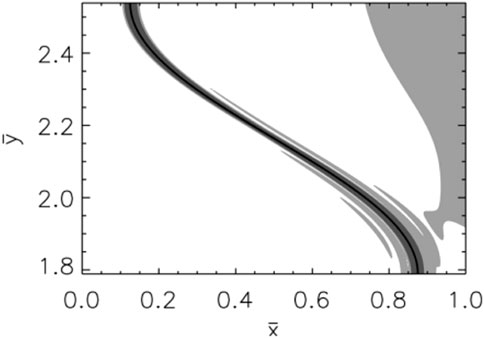
FIGURE 1. Fourth panel from Figure 3 of Russell and Wright (2010). Result from a numerical simulation of FLR, showing accumulation of energy density along a resonant contour in the (x, y) plane.

These studies have all used uniform, straight magnetic fields. A critical aspect of more realistic magnetic geometries which is therefore ignored in these works is that the Alfvén frequency of a field line varies with the wave polarisation. That is to say, a poloidal Alfvén wave and a toroidal Alfvén wave of the same field line have different frequencies (Dungey, 1954; Radoski, 1967; Cummings et al., 1969). This occurs due to the different convergence of magnetic field lines in the directions perpendicular to the field, and will become apparent from the Alfvén wave equation developed later in this review. This difference in frequency underpins most of the research which is to follow, and therefore it is appropriate to introduce this idea as thoroughly and explicitly as possible.

Consider a fixed global fast driving frequency, ω_d. In a straight background magnetic field, there will be a resonant field line at a given L-shell (where L labels the set of field lines which cross the magnetic equator at a radial distance equal to L), say L_r, such that the resonance condition ω_A (L_r) = ω_d, for Alfvén frequency ω_A, is satisfied. This location is unique i.e. the FLR exists at one radial location (assuming a density profile such that there is a monotonic variation of ω_A(L)). However, in a dipole field the Alfvén frequency depends on the wave polarisation, and permits many L-shells to satisfy the resonance condition simultaneously. In other words, the L-shell for which a toroidal Alfvén wave polarisation satisfies the resonance condition will be different from the L-shell for a poloidal Alfvén resonance. This enforces a resonant region (rather than a single location), which is termed the Resonant Zone, over which FLRs can exist (Wright and Elsden, 2016). The polarisation of resonant Alfvén waves varies smoothly over this region, and therefore there exists an infinite family of solutions to the 3-D resonance problem. The question then becomes, which of these solutions are relevant for a given equilibrium?

In the sections which follow, we will develop the different models which have yielded answers to the above question, building in complexity. The review is structured as follows: Section 2 discusses the analysis of 3-D FLRs in 2-D and 3-D dipole magnetic field geometries using orthogonal field-aligned coordinate systems; Section 3 treats more general magnetic fields using non-orthogonal field-aligned coordinates; Section 4 considers analytical efforts to find approximate solutions to the 3-D FLR problem; Section 5 summarises the current state of this field and discusses future research directions and unanswered questions.

2 3-D Alfvén resonances in dipole magnetic fields

2.1 2-D (Line) dipole with a 3-D density profile

2.1.1 Model setup

We begin with the simplest modelling configuration to highlight the implications of the Alfvén frequency variation with polarisation. In this section, we consider a 2-D dipole magnetic field which is invariant in z, together with a 3-D density variation to provide a 3-D inhomogeneous medium. A 2-D dipole magnetic field provides a significant difference in the toroidal and poloidal Alfvén frequencies of a field line (in fact more than the 3-D dipole (see pg. 126 Elsden, 2016)). The 2-D dipole can be pictured as a 3-D dipole which has been unfurled and straightened out in the azimuthal direction, such that there is no variation in the magnetic field with azimuth. A field-aligned coordinate system can naturally be prescribed to such a potential dipole field, by defining the magnetic field in terms of a scalar potential ψ and vector potential A such that $\mathbf{B}=\nabla \psi =\nabla \times \left(A{\mathbf{e}}_{\mathbf{z}}\right)$. In standard cylindrical polar coordinates (R, ϕ, z) this yields

$\psi =\frac{B_0{R}_0^2}{R}\sin \varphi ,(1)$

$A=\frac{A_0{R}_0}{R}\cos \varphi ,(2)$

with A as the z-component of the vector potential A and at (R, ϕ) = (R₀, 0), the background magnetic field strength B = B₀ and A = A₀ = B₀R₀. Unfortunately, these ‘standard’ 2-D dipole coordinates are very poorly suited for numerical computations. Equal steps in the value of each coordinate yield vastly different distances in real space at different points along the field line. Therefore a uniformly spaced numerical grid based on these coordinates will dramatically under-resolve certain regions, and over-resolve others, as very well explained and visualised by Kageyama et al., 2006, Figure 2). To overcome this, alternative spatial coordinates that are functions of the standard coordinates, α(A), β = z, γ(ψ), can be adopted which maintain the dipole field structure but greatly improve the resulting grid spacing used for numerical modelling. The specific functions are listed in Wright and Elsden (2016), Equation 5, where α is the meridional coordinate labelling L-shells, β is the straight azimuthal direction (z-axis in cylindrical coordinates) and γ is the field-aligned coordinate. These coordinates (α, β, γ) form an orthogonal field-aligned coordinate system. A view of a meridional plane explaining the coordinates is displayed in Figure 2A. The blue circles indicate lines of constant α i.e., magnetic field lines. The field-aligned coordinate γ is constant along the red lines. Choosing suitable minimum and maximum values of these coordinates would specify the numerical solution domain.

FIGURE 2

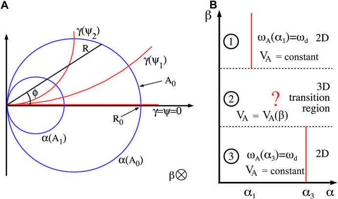
FIGURE 2. (A) Schematic in a meridian plane of the 2-D dipole coordinates (α, β, γ) used in the model (Figure 2, Wright and Elsden (2016)). (B) View looking down on the equatorial plane of the 2-D dipole, considering how the resonance location might vary for a medium which varies with azimuth (β), further explained in the main text (Figure 1, Wright and Elsden (2016)).

Figure 2B explains a thought experiment Wright and Elsden (2016) used to begin formulating their understanding of the 3-D Alfvén resonance process. The figure shows a view from above of the equatorial (α, β, γ = 0) plane, with three distinct regions labelled, where the plasma mass density (and therefore Alfvén speed) varies between them. In regions one and three, the density is constant but different between the regions, with a larger density in region one than three. In region two, the density varies smoothly to connect the different densities either side. Consider applying a constant monochromatic driver, of frequency ω_d, or equally looking for normal mode solutions proportional to $e^{i{\omega }_{d}t}$. In regions one and three, it is well known from previous works that FLRs will form at locations α₁ and α₃ as labelled (the red lines), where the local Alfvén frequency matches the driving frequency. This occurs further radially inward at region one due to the increased density there lowering the Alfvén frequencies, and therefore the resonance will occur on shorter field lines than in region three. Furthermore, the polarisation of the magnetic and velocity fields associated with the Alfvén wave will be toroidal, i.e., in the azimuthal (β) direction. These are labelled as ‘2-D’ FLRs, because in these regions there is no variation in the medium with azimuth. However, the question of interest is what occurs in region two? Here the medium is varying azimuthally due to the density change and hence is labelled 3-D. Where will FLRs form? What polarisation will they have? Can they be excited as efficiently as their 2-D counterparts?

2.1.2 Normal mode simulations

To answer such questions, Wright and Elsden (2016) design an equilibrium based on the variation of the density with azimuth as shown in region two in Figure 2B, to provide a fully 3-D medium. The linear, cold (low β), MHD equations, cast in the field-aligned coordinate system previously described, are solved numerically (see , Wright and Elsden (2016)). In the first instance, steady-state oscillatory solutions (normal modes) are considered, assuming a time dependence of the form $e^{i{\omega }_{d}t}$. The field-lines are fixed into a perfectly conducting ionosphere, imposed by setting nodes of displacement at each end of the field line.

Figure 3A (reproduced from Figure 7 of Wright and Elsden (2016)) displays a shaded surface plot of the time-averaged energy density from the simulation, in the equatorial (α, β, γ = 0) plane. This quantity is used as an indication of Alfvén resonance formation, given the expectation that significant energy should accumulate at resonant field lines. There is a clear enhancement of the energy density along a particular path. Furthermore, it was shown that the velocity and magnetic fields are polarised along (or equally can be thought of as being tangential to) this path (see Figure 4 of Wright and Elsden (2016)). That is to say, the Alfvén waves forming the FLR have an intermediate polarisation between poloidal and toroidal, similar to the studies which used the box model (Lee et al., 2000; Russell and Wright, 2010). Other hallmarks of Alfvén resonance are also borne out, such as the amplitude and resonance width scaling as expected with the provided dissipation in the model.

FIGURE 3

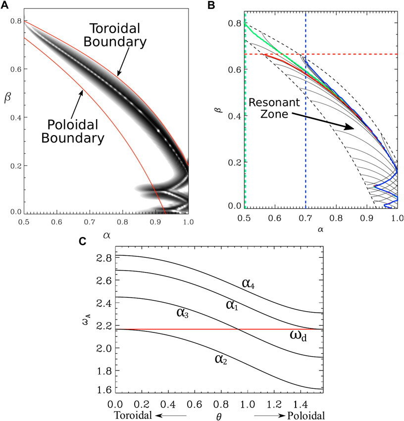
FIGURE 3. Reproduction of Figure 7 from Wright and Elsden (2016). (A) Shaded surface of the total energy density in the equatorial (α, β) plane from a normal mode simulation. Red lines are the poloidal and toroidal Resonant Zone boundaries. (B) Resonance map with solid black lines representing solutions satisfying the Alfvén resonance condition. Red, blue and green solid lines give the dominant solution paths for different boundary conditions and boundary locations (dashed colored lines) as further explained in the main text. (C) Variation of Alfvén frequency ω_A with polarisation angle θ for four field lines at different radial distances labelled α₁…α₄. The red line gives the fast driving frequency ω_d (adapted from Figure 6 of Wright and Elsden (2016)).

To analyse the results further, one requires the ability to calculate the Alfvén frequency for an intermediate polarisation of Alfvén wave. An Alfvén wave equation for the separate poloidal and toroidal modes can be derived from the full linear MHD equations by assuming negligible magnetic field compression, or in the previously described system, b_γ = 0. Several authors have discussed these Alfvén wave equations (Radoski, 1967; Cummings et al., 1969; Singer et al., 1981) but we present them here in the form given by Wright and Thompson (1994) as:

$\frac{\partial }{\partial \gamma }\left(\frac{1}{h_{\gamma }}\frac{\partial U_{\alpha }}{\partial \gamma }\right)+\frac{1}{h_{\gamma }}\frac{\partial }{\partial \gamma }\left(\ln \left(\frac{h_{\alpha }}{h_{\beta }}\right)\right)\frac{\partial U_{\alpha }}{\partial \gamma }+\frac{{\omega }_A^2}{V_A^2}{h}_{\gamma }{U}_{\alpha }=0,(3)$

$\frac{\partial }{\partial \gamma }\left(\frac{1}{h_{\gamma }}\frac{\partial U_{\beta }}{\partial \gamma }\right)+\frac{1}{h_{\gamma }}\frac{\partial }{\partial \gamma }\left(\ln \left(\frac{h_{\beta }}{h_{\alpha }}\right)\right)\frac{\partial U_{\beta }}{\partial \gamma }+\frac{{\omega }_A^2}{V_A^2}{h}_{\gamma }{U}_{\beta }=0(4)$

Where the quantities U_α and U_β, used in the simulations of Wright and Elsden (2016), are related to the transverse velocity components (u_α and u_β) by U_α = u_αh_βB, U_β = u_βh_αB. The scale factors are given by h_α, h_β, h_γ such that a length element dr in real space can be written as

$\mathbf{d}\mathbf{r}=h_{\alpha }d\alpha {\mathbf{e}}_{\alpha }+h_{\beta }d\beta {\mathbf{e}}_{\beta }+h_{\gamma }d\gamma {\mathbf{e}}_{\gamma }.(5)$

The background magnetic field strength is B and the Alfvén speed is V_A. The Alfvén frequency for a field line depends on the transverse coordinates, i.e., ω_A (α, β). Notice that the derivatives are purely with respect to the field-aligned direction, γ. The discrepancy in the poloidal and toroidal equations arises from the difference between the perpendicular scale factors h_α and h_β. If these were the same (e.g. in a straight background magnetic field), then the poloidal and toroidal Alfvén frequencies would be equal. In the 2-D dipole geometry however, h_α and h_β differ substantially along a field line which creates the different poloidal and toroidal frequencies.

A key extension of these equations was derived by Wright and Elsden (2016) to allow for the calculation of the frequency of Alfvén waves of intermediate (between poloidal and toroidal) polarisation. The authors showed how to calculate the scale factors for a new transverse coordinate system (α′, β′) that is rotated about the field-aligned direction in the equatorial plane by the polarisation angle, θ. In this way the β′ coordinate could be oriented along the resonance and so align with the Alfvén wave displacement. This permits the rewriting of the Alfvén wave equation as:

$\frac{\partial }{\partial \gamma }\left(\frac{1}{h_{\gamma }}\frac{\partial U_{{\beta }^{\prime }}}{\partial \gamma }\right)+\frac{1}{h_{\gamma }}\frac{\partial }{\partial \gamma }\left(\ln \left(\frac{h_{{\beta }^{\prime }}}{h_{{\alpha }^{\prime }}}\right)\right)\frac{\partial U_{{\beta }^{\prime }}}{\partial \gamma }+\frac{{\omega }_A^2}{V_A^2}{h}_{\gamma }{U}_{{\beta }^{\prime }}=0,(6)$

where h_α′, h_β′ are the scale factors for the rotated coordinate system (specific forms given by Eqs. 22, 20 respectively, of Wright and Elsden (2016)) and U_β′ = u_β′h_α′B is related to the velocity perturbation along the resonant contour (u_β′). The Alfvén frequency can now be regarded as a function of not only the field line it is on (i.e., α and β), but also the orientation of the resonance (θ), i.e., ω_A (α, β, θ).

Figure 3B and the red lines in Figure 3A may now be explained. We can pose the question: if the polarisation angle θ is fixed to be poloidal (θ = π/2) or toroidal (θ = 0), for the given equilibrium, where will the resonance condition (Alfvén frequency equal to fast driving frequency) be satisfied? The solutions are the red lines in Figure 3A. Along the outer (right) red line, a toroidal Alfvén wave polarisation will satisfy the resonance condition, or in the previously stated notation ω_A (α, β, θ = 0) = ω_d. Along the inner (left) red line, a poloidal Alfvén wave polarisation will be be resonant (ω_A (α, β, θ = π/2) = ω_d). These lines bound what is termed the Resonant Zone (Wright and Elsden, 2016), as only within this region can FLRs occur. Equally, outside of this region no polarisation of Alfvén wave exists such that the Alfvén frequency matches the driving frequency.

This can be well visualised by plotting the Alfvén frequency (ω_A) variation with polarisation angle (θ), as shown in Figure 3C. The black lines show this variation for four field lines at different radial locations in the equatorial plane (labelled α₁…α₄) but in the same meridian plane (i.e., β is constant). The constant fast driving frequency (ω_d) is given by the red line. The Alfvén frequency smoothly decreases from a maximum for a toroidal polarisation (θ = 0) to a minimum for poloidal (θ = π/2). For field line α₁, it can be seen that a poloidal polarisation is required to match the driving frequency, while a toroidal polarisation is needed for α₂ to be resonant. These requirements mark these field lines as the locations of the poloidal (α₁) and toroidal (α₂) Resonant Zone boundaries for this magnetic local time (β = const.), where α₁ < α₂ i.e. α₁ is further radially inward. Considering the field line labelled α₄, radially inward of α₁, the Alfvén frequency is greater than the driving frequency ω_d for all polarisations. Therefore, for field lines radially inward of α₁ and radially outward of α₂, no polarisation exists to satisfy the resonance condition (assuming a suitable monotonic variation of ω_A with α). The maximum/minimum frequencies coinciding with the toroidal/poloidal polarisations is a feature of the purely dipolar magnetic field and does not occur for more general magnetic field geometries, as will be treated in later sections.

Inside the Resonant Zone, at any given point, what polarisation of Alfvén wave is required to satisfy the resonance condition? Choosing a starting field line, for example α₃ in Figure 3C, one can find the polarisation (θ) which gives an Alfvén frequency matching the driving frequency. Wright and Elsden (2016) explain how the FLR follows a path in the equatorial plane whose tangent coincides with this polarisation. If, in the equatorial plane, the coordinates α and β correspond to physical space, then the path of the FLR there will satisfy the equation

$\frac{\mathrm{d}\alpha }{\text{d}\beta }=\tan \left(\theta \right),(7)$

which follows from the definition of the polarisation angle θ being measured from the β axis. Inverting the resonance relation

${\omega }_A\left(\alpha ,\beta ,\theta \right)={\omega }_d(8)$

to give θ(α, β, ω_d), it is evident that Eq. 7 can be solved for a given ω_d. The solutions correspond to resonant paths and are shown by the black lines in Figure 3B. There are in fact an infinite number of solutions within this domain, and the lines drawn are chosen to represent the overall character of the solutions. It can be seen that these lines emerge from the poloidal boundary with zero gradient in the (α, β) plane, and approach the toroidal boundary with infinite gradient. This reflects the fact that the transverse magnetic and velocity perturbations are polarised tangential to these paths, so emerge from the poloidal boundary with, unsurprisingly, a poloidal polarisation and similarly for the toroidal boundary. Between these boundaries, all solutions have an intermediate polarisation between poloidal and toroidal, as per the solution found for the particular field line as in Figure 3C. For any field line in the Resonant Zone of a dipole field there exist solutions for both positive and negative polarisation angles (±θ) and this leads to the crossing of contours where such paths are drawn. Otherwise, the contours are nested.

Any one of these solutions paths is mathematically viable, so how can the preferred path shown by the enhanced energy density in Figure 3A be explained? This path is overlaid as the solid green line in panel (b). For this simulation, the inner boundary was placed at α = 0.5, denoted by the dashed green line. At this boundary, a condition of perfect reflection or no flow across the boundary (u_α = b_α = 0) was applied. This means that any perturbation existing at the boundary can only have a toroidal perturbation. Therefore the dominant resonant path is the one which emanates from the location where the toroidal boundary intersects the simulation boundary, i.e., the solid green line. This theory was tested by performing two other simulations with different boundary locations. Moving the inner boundary to α = 0.7 (blue dashed line) enforces a toroidal polarisation there, resulting in the blue path being the location of enhanced energy density (energy density plot not shown here). When the boundary in β is moved to β = 0.67 (red dashed line), with the condition of a zero azimuthal perturbation there, this enforces a poloidal perturbation, such that the solid red line becomes the favoured solution path. Therefore it is clear that boundary conditions play an important role in the FLR selection process.

Another important feature identified in the simulations of Wright and Elsden (2016) was the effect of locally 2-D regions where the azimuthal derivatives of the equilibrium vanish. Figure 4 is a reproduction of Figure 10 from Wright and Elsden (2016), showing results from a simulation with an equilibrium designed to highlight this. The background Alfvén speed profile has been tailored to be invariant in azimuth for |β| > 0.2, and increases smoothly towards β = 0, where azimuthal derivatives are also zero. This increases the Alfvén frequency in this region (|β| < 0.2) and forces the Resonant Zone further radially outwards to longer field lines. The peaks in the energy density in Figure 4A clearly show a strong toroidally polarised FLR in the 2-D regions, evident by the dark peaks on the toroidal (outer red line) boundary. These solution paths then connect to 3-D FLRs (of intermediate polarisation) in the middle region where V_A varies azimuthally. The contours appear to be reflected off the toroidal zone boundary, switching between solutions (as was also evident in Figure 3A). At the peak of the toroidal boundary at (α, β) = (0.92, 0.0), the Alfvén frequency is invariant with azimuth (∂/∂β = 0), and further seems to seed solution paths which emanate from this point. Indeed, in simulations where the extended 2-D, azimuthally invariant regions are not included, it is the locally 2-D regions which seed all of the excited resonant paths (see Figure 8, Wright and Elsden, 2016). Therefore such locally 2-D regions appear to be important for selecting the dominant solution, a theory which is generalised later in this review. Figure 4B displays the Resonance Map for this equilibrium and driving frequency. There is a clear convergence of solutions onto those selected in the simulation shown in panel a).

FIGURE 4

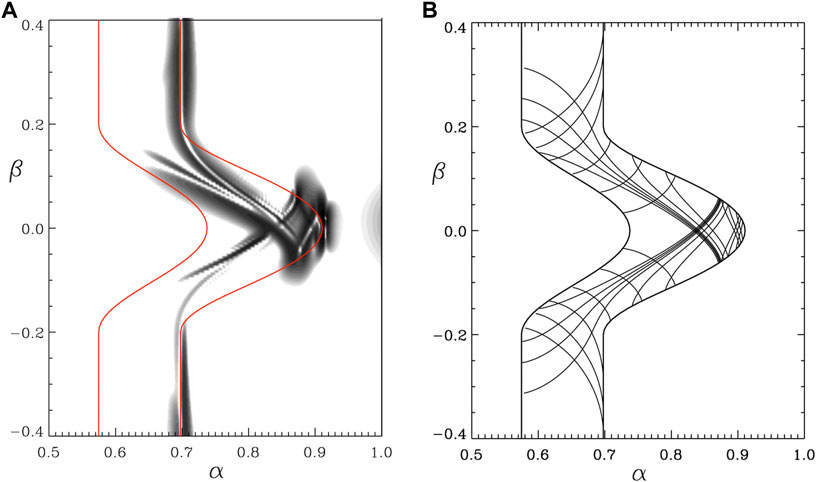
FIGURE 4. Figure 10 from Wright and Elsden (2016). (A) Shaded surface of the total energy density in the equatorial plane. Red lines are the boundaries of the Resonant Zone. (B) Resonance Map for simulation equilibrium and chosen driving frequency.

The governing equations may be cast as coupled wave equations, as shown in Equation 9 of Wright (1992). The left hand side is the Alfvén wave operator (in their case for b_β) and the right hand side represents a driving term associated with magnetic pressure. From a mathematical perspective, the Alfvén wave equations shown in Eqs. 3, 4, 6 are the homogeneous form of the driven Alfven wave equations, and their oscillatory solutions are Alfvénic normal modes representing the free oscillations of field lines corresponding to the complementary function. Overall, it is clear that the Resonance Map (based on these complementary functions) is an excellent indicator of the location and polarisation of FLRs for a given driving frequency.

2.1.3 Time-dependent simulations

The previous section treated the steady-state solution, by assuming that all components had a time dependence proportional to $e^{i{\omega }_{d}t}$. However, it is of great interest to understand how the system evolves to reach such a state. There has been a rich history in 1-D/2-D resonance theory of the study of time-dependent features such as Alfvén wave phase mixing (Burghes et al., 1969; Heyvaerts and Priest, 1983) and resonance widths (Mann et al., 1995; Smith et al., 1998). Therefore an important step is to examine these properties in the 3-D resonance setting. Figure 5 displays results from time-dependent simulations by Elsden and Wright (2017), using the same equations and 2-D dipole coordinates as discussed above. The equilibrium is set up similarly to that presented in Figure 2B, where there are two azimuthally invariant regions either side of the ‘3-D’ region where the density varies with azimuth. The outer boundary of the simulation is driven continuously through monochromatic perturbations of the field-aligned magnetic field component, b_γ. This simulates driving with magnetic pressure, modelling the effect of the solar wind buffeting the magnetopause.

FIGURE 5

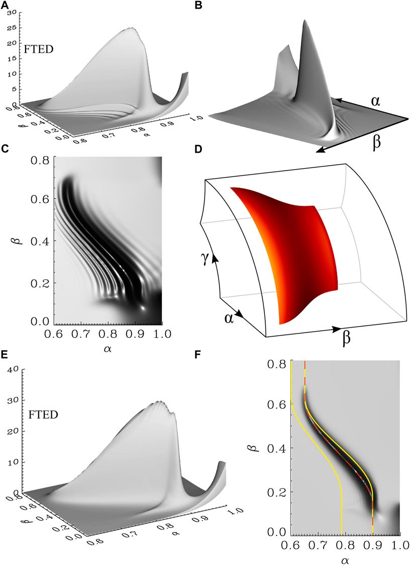
FIGURE 5. Composite of Figures 4, 5, Elsden and Wright (2017). (A) Shaded surface of flux tube energy density (FTED) at an early simulation time. (B) Rotated view of (A). (C) Aerial view of (A). (D) Surface of resonant field lines (orange) in real space within the dipole simulation domain skeleton. (E) Shaded surface of FTED for a later simulation time. (F) Aerial view of (E) together with the Resonant Zone boundaries (yellow) and favoured resonant path (red dashed).

The grey plots in Figure 5 each display a shaded surface of the flux tube energy density (FTED, i.e., the energy contained in a flux tube of unit cross section in the equatorial plane) from different orientations and simulation times. Panel (a) shows a snapshot at an early time in the simulation in the equatorial plane, with the driven outer boundary being at the back right hand edge of the plot at α = 1.0. A peak in the energy density has formed, clearer in panel (b) which simply shows a rotated view of (a). The amplitude decreases away from the driven boundary and nested ‘ridges’ appear either side of the main peak. Panel (c) shows a view from above which further highlights these ridges in the energy density. Panel (d) displays the simulation domain in real space, with the orange surface representing the sheet of field lines corresponding to the energy density peak.

The bottom panels (e) and (f) are taken from near the end of the simulation, once a steady state has been reached after continuous monochromatic driving. This state is the same as the normal modes described in the previous subsection. The shaded surface plots clearly show that the ridges in the energy density have disappeared, with one preferred solution path remaining. We can summarise the results from this plot and further analysis by Elsden and Wright (2017) not shown here as follows:

• The amplitude peak is indeed a resonant response, as can be determined by the secular growth in time (prior to saturation) of the velocity/magnetic field components polarised along the main ridge.

• The path selected by the resonance agrees with the theory from the previous section, that it is precisely the path which connects the toroidally polarised regions at β < 0.15 and β > 0.6, as can be seen from the red dashed line in Figure 5F.

• The ridges in the energy density (best observed in Figure 5C) form due to phase mixing - the process by which oscillations of field lines of different natural frequencies drift out of phase over time. At early times, the bandwidth of the established fast mode in the domain is large due to the short duration of driving. Therefore many field lines respond resonantly to this broadband signal. By later times, once the fast frequency bandwidth within the domain has narrowed, only the surface of field lines (panel (d)) matching this frequency are resonant (panel (f)).

• The spatial separation of the ridges, and indeed the steady state resonance width, are shown to be governed by the phase mixing length and the dissipation time. The phase mixing length is an estimate of the local wavelength perpendicular to the ridges in energy density, and a 3-D extension to this is provided by Elsden and Wright (2017) (their Eq. 19). There will further be a phase motion from high to low Alfvén frequency (Wright et al., 1999), which in the case of Figure 5C can be pictured as the ridges propagating outward, normal to the ridges.

• Elsden and Wright (2017) provide a formula for the 3-D resonance amplitude (see their Eq. 25), as an extension to the previous 2-D theory. The amplitude has an inverse dependence on the perpendicular Alfvén frequency gradient, perhaps counter-intuitively, such that sharper gradients lead to smaller resonance amplitudes. The amplitude is limited by the presence of dissipation in the system.

Thus far, focus has only been given to the 3-D Alfvén resonance structure and not to the other key aspect of FLR, which is the fast mode which drives it. In a series of papers, Elsden and Wright (2018); Wright et al. (2018); Elsden and Wright (2019) considered the effect of the temporal and spatial structure of the fast mode on the resulting Alfvén resonance, again in the 2-D dipole magnetic field geometry. This is not the focus of this review, but it is worth mentioning the generalisation of the fast mode driving condition to 3-D. In 2-D, azimuthal gradients are required in the fast mode to drive Alfvén resonances (e.g., see the right hand side of Equation 2 of Wright (1994)). This is equivalent to the statement that the fast and Alfvén modes are decoupled for fast modes with azimuthal wavenumber m = 0. In 3-D, this condition for Alfvén resonance becomes that gradients in the fast mode are required in the direction tangential to the resonant path.

2.2 3-D Dipole

The natural extension to the studies in the previous section is to consider a background 3-D magnetic dipole, such that more realistic equilibria may be studied. Wright and Elsden (2020) have designed a numerical model based on such a field structure, in a similar manner to the 2-D dipole. They cast the linear MHD equations in field-aligned coordinates based on the 3-D dipole, again optimised for numerical efficiency. The workings and equations are omitted here for brevity, but Eqs. 27–31 of Wright and Elsden (2020) list the partial differential equations solved in their model.

Figure 6A displays the equilibrium Alfvén speed from the simulation. A depression in the Alfvén speed has been included on the dusk flank to model the effect of a plasmaspheric plume: an extension of the dense plasmasphere around dusk associated with geomagnetic disturbances (e.g., Goldstein et al., 2005). Such azimuthal inhomogeneity should provide the perfect conditions for 3-D Alfvén resonances based on the ideas developed in the previous section. An impulsive broadband variation to the field-aligned magnetic field component b_γ, is applied to the magnetopause (the outer simulation boundary) to drive the model. A late-time snapshot of the resulting field-aligned current density j_γ close to the ionospheric end of the field lines, mapped to the equatorial plane for visualisation, is displayed in Figure 6B. The field-aligned current density is used as a proxy for the Alfvén wave, since fast waves do not carry a strong field-aligned current. There is a clear dawn-dusk asymmetry induced by the asymmetry in the equilibrium. At dawn, where the equilibrium is locally 2-D, the phase-mixed resonant ridges align with the dashed black reference circles at constant L-shell. From the previous section, we know that this implies toroidally polarised FLRs in this region (velocity/magnetic field perturbations are tangential to the circles). At dusk however, upon encountering the change in the equilibrium with azimuth, the ridges of Alfvén wave current are diverted radially inwards, crossing around two L-shells (as is clear from the black dashed circles). The Alfvén frequency is constant along any one of these ridges, and the polarisation changes in such a manner to maintain this same frequency.

FIGURE 6

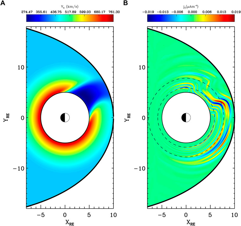
FIGURE 6. Reproduction of Figure 11 from Wright and Elsden (2020). (A) Contour of Alfvén speed in the equatorial plane. (B) Contour of field-aligned current density j_γ close to the ionospheric end of the field line, mapped to the equatorial plane. Black dashed lines are at constant L-shell, at 6 and 8 R_E for reference.

3 Compressed dipole and more general magnetic fields

The purpose of this section is to extend our consideration from the 3-D dipole background magnetic field to more general and realistic field line geometries in which azimuthal (and ultimately all) symmetries are removed. This is necessary to consider the effects of the increased distortion of magnetic field lines from a dipole configuration under equilibrium conditions as L-shell is increased. For example, field lines become distorted as their proximity to the magnetopause is reduced along the dayside and dawn/dusk flanks, and magnetotail stretching becomes important on the nightside. As before, we wish to use a coordinate system in which one of the coordinates is aligned with magnetic field lines. To do this, we require coordinates $\left(\alpha ,\beta ,\gamma \right)$, such that γ measures position along field lines, while α and β measure position strictly across field lines. This is given by Euler Potential coordinates (Stern, 1970) α(x, y, z) and β(x, y, z), such that the vector potential for the background magnetic field is A = α∇β, in which case B = ∇ ×A = ∇α ×∇β. The field-aligned coordinate can in principle be any function that strictly increases along all closed magnetic field lines from the foot-point at one hemisphere to the other.

Globally defined field-aligned coordinate systems are in general non-orthogonal for magnetic fields that lack specific physical/topological properties (Salat and Tataronis, 2000). The key ingredients required for orthogonal field-aligned coordinates are: a) There are no field-aligned currents (in which case B ⋅∇×B = 0, and the magnetic field can be expressed as B = σ∇γ where σ is a scalar variable, and hence ∇α ⋅∇γ = ∇β ⋅∇γ = 0), and b) there is no magnetic shear $\widehat{s}$ (where $\widehat{s}\propto \left(\mathbf{B}\times \nabla \psi \right)\cdot \nabla \times \left(\mathbf{B}\times \nabla \psi \right)$, and ψ = ∫_SB ⋅ dS is the magnetic flux passing through a defined surface S). If the magnetic field topology is such that field lines with the same ψ form nested surfaces, then these can be used as the Euler potential coordinate α, and β can be defined as an angle-like coordinate (for example, the azimuthal angle ϕ). In this case it can be shown that $\widehat{s}\propto \partial /\partial \gamma \left(\nabla \alpha \cdot \nabla \beta /\nabla \alpha \cdot \nabla \alpha \right)$, therefore a necessary condition for the existence of orthogonal α and β coordinates (such that ∇α ⋅∇β = 0) is that $\widehat{s}=0$. This precludes, for example, magnetic field models that seek to account for day-night asymmetry within Earth’s magnetosphere from being described globally by an orthogonal coordinate system, even vacuum magnetic field models (Mead, 1964; Stern, 1985), since these have nonzero magnetic shear.

Two different approaches have historically been used to deal with the MHD wave equations in non-orthorgonal curvilinear coordinate systems. One approach developed by Cheng et al. (1993); Cheng (2003); Cheng and Zaharia (2003) is to use the directions given by B, ∇ψ and B ×∇ψ to define locally orthogonal vector components. These are then used to express the governing MHD wave equations. Some simplifications are provided by identifying terms relating to magnetic field properties, such as magnetic shear, and components of the field line curvature ($\kappa =\widehat{\mathbf{B}}\cdot \nabla \widehat{\mathbf{B}}={\nabla }_{\perp }\left({\mu }_{0}P+B^2/2\right)/B^2$, where $\widehat{\mathbf{B}}=\mathbf{B}/|\mathbf{B}|$, B² = B ⋅B and P is the equilibrium pressure). Some of the analytical results for field line resonances using this method are discussed in .

The other common approach has been to use the contravariant/covariant formalism (Lysak, 2004; Rankin et al., 2006; Kabin et al., 2007; Degeling et al., 2010; 2018), which is described in D’haeseleer et al. (1991). Briefly, a vector (say V) can be described in terms of either covariant or contravariant (reciprocal) basis vectors, denoted e_i = ∂R/∂uⁱ and eⁱ = ∇uⁱ respectively, where R is the position vector and uⁱ denote coordinate labels, e.g., α, β and γ (as i increases from 1 to 3). For example, V = V_ieⁱ = Vⁱe_i (note that repeated indices imply summation), and the covariant (contravariant) components are given by V_i = V ⋅e_i (Vⁱ = V ⋅eⁱ). The two sets e_i and eⁱ are known as reciprocal basis vector sets, and satisfy the relation ${\mathbf{e}}^i\cdot {\mathbf{e}}_j={\delta }_j^i$ (the Kronecker delta function, equal to one if i = j and zero otherwise). It can be shown that one set of basis vectors can be used to give the other, with e_i = e^j ×e^k/(eⁱ ⋅e^j ×e^k) and similarly eⁱ = e_j ×e_k/(e_i ⋅e_j ×e_k) (where i, j, k cycle through 1,2,3). The terms appearing in the denominators are Jacobians of the forward and reverse transformations between eⁱ and e_i, hence they have a reciprocal relationship: $J={\mathbf{e}}_i\cdot {\mathbf{e}}_j\times {\mathbf{e}}_k={({\mathbf{e}}^i\cdot {\mathbf{e}}^j\times {\mathbf{e}}^k)}^{-1}$. The geometric properties of the coordinate system are characterized by the covariant (contravariant) metric coefficients g_ij = e_i ⋅e_j (g^ij = eⁱ ⋅e^j), and allow one set of vector components to be determined from the other, for example V_i = g_ijV^j and Vⁱ = g^ijV_j. This also implies that $g^{ij}{g}_{ij}={\delta }_j^i$; hence (treating these as 3 × 3 matrices) that $[g_{ij}]={[g^{ij}]}^{-1}$, and it can be shown that $\det \left([g_{ij}]\right)\equiv g=J^2$. With these definitions, B = ∇α ×∇β = B^γe_γ, where $B^{\gamma }={\mathbf{e}}^{\alpha }\times {\mathbf{e}}^{\beta }\cdot {\mathbf{e}}^{\gamma }=1/\sqrt{g}$, and the other contravariant components of B are zero. Note that if the coordinate system is orthogonal, then [g_ij] is diagonal, with the nonzero terms giving the square of the orthogonal coordinate scale factors: $g_{ii}=h_i^2$, and also $\sqrt{g}=h_{\alpha }{h}_{\beta }{h}_{\gamma }$.

The works of Rankin et al. (2006); Kabin et al. (2007) and Degeling et al. (2010, 2018) stem from the linearized ideal MHD equations for a cold plasma, given by:

$\frac{\partial \mathbf{b}}{\partial t}=-\nabla \times \mathbf{E}(9)$

$\frac{1}{V_A^2}\frac{\partial \mathbf{E}}{\partial t}={\nabla }_{\perp }\times \mathbf{b}-\frac{\left({\mu }_0\mathbf{J}\times \mathbf{b}\right)\times \mathbf{B}}{B^2}(10)$

where b and E are the first order perturbations of the magnetic and electric fields, and μ₀J = ∇ ×B is the background current density. Note that the above equations are strictly valid from the point of view of maintaining an MHD equilibrium in background conditions only when J ×B = 0, in which case either ∇ ×B ∝B (only field aligned currents) or B = ∇γ (“vacuum” magnetic field; no currents allowed), otherwise a background pressure gradient is required for equilibrium, which allows coupling to MHD slow mode waves. (This is taken into account in the comprehensive work of Cheng (2003) mentioned earlier).

Writing Eqs. 9, 10 in (α, β, γ) component form gives (Rankin et al., 2006) a set of five first-order partial differential equations (PDEs) for E and b (with E_γ = 0 for ideal MHD). Setting b_γ = 0 and assuming variations of the form exp (−iωt) reduces these to ordinary differential equations (ODEs) with respect to γ for shear Alfvén wave (SAW) eigenmodes of frequency ω in which the polarization is unspecified a-priori, but is a function of the local magnetic field topology, specified by the metric coefficients g^ij. This is explored in detail in Kabin et al. (2007) for the fundamental modes and Kabin et al. (2009) for higher harmonics, using an analytic compressed dipole magnetic field (for which the Euler potential coordinates and metric coefficients can be expressed in closed form). For these studies the plasma density is axisymmetric and the loss of axisymmetry in the wave equations is only due to the magnetic field model, not the plasma density.

Examples of the results of this calculation for the two lowest frequency eigenmodes on each field line are shown as maps in the equatorial plane in Figure 7. Both of these modes correspond to fundamental transverse oscillations with respect to the field-aligned direction, with the left (right) column corresponding to the nominal toroidal (poloidal) SAW eigenmodes for r < 3R_E where the background magnetic field is approximately dipolar. As radius increases, the top row of plots show that the eigenfrequencies of both modes lose their axisymmetry, becoming misaligned with contours of constant |B| (indicated by solid black lines). Meanwhile the bottom row shows that the polarization directions of these modes become increasingly altered from the dipolar case with increasing L-shell, especially on the dayside where the background magnetic field is compressed. Along the noon meridian, the polarization changes discontinuously at r ≈ 5 from radial to azimuthal in Figure 7C) and visa-versa in Figure 7D). This corresponds with a point of degeneracy in the eigenfrequencies of the two modes. In plots c) and d), the eigenmode calculations are carried out at locations corresponding to contours of constant |B| (the midpoint of each double-headed arrow in the plots). Following such a contour starting at noon for r > 5 and proceeding to midnight, the polarization is shown to smoothly rotate by π/2 radians in both figures.

FIGURE 7

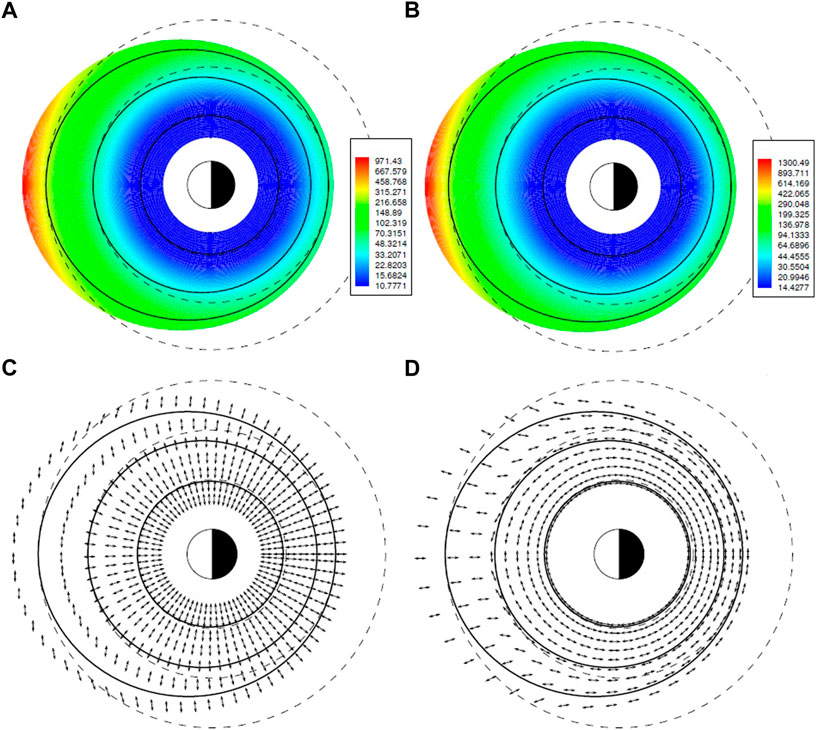
FIGURE 7. Eigenperiods and electric field polarizations in the equatorial plane for the two lowest frequency Alfvénic eigenmodes, taken from Figures 3, 6 of Kabin et al. (2007): (A) Period and (C) polarization of the mode with radial electric field polarization at midnight; (B) Period and (D) polarization of the mode with azimuthal electric field at midnight. Thick solid lines show the contours of constant B initiated at r = 3, 5, and 7 at noon. Dashed lines are circles of constant radius with r = 3, 5, and 7. Note the sudden change in the polarization along the noon meridian at r ≈ 5 in (C,D). This occurs at a point of degeneracy in the eigenperiod in (A,B).

A similar rotation of polarization for each mode would be found following a surface of constant eigenfrequency. This is important because it indicates a limit in the physical applicability of the eigenmode solutions in a global context: Each eigenmode remains independent of oscillations on neighboring field lines, as long as b_γ is zero. However, given the eigenmode polarizations specified by the magnetic topology are in general not aligned with contours of constant eigenfrequency, phase mixing of oscillations between these surfaces will lead to equatorial electric field patterns that are unable to remain curl-free - and give rise to a first order b_γ. This strongly suggests that an additional constraint on the polarization (namely, that the equatorial electric field remains curl-free) must be be applied in the calculation of 3‐D Alfvénic eigenfunctions.

This is borne out in the model results of Degeling et al. (2010), in which the coupled wave equations (Eqs. 9, 10) are expressed using the covariant/contravariant formalism and solved numerically. In this work the background magnetic field is defined by B = σ∇γ, in which case g^αγ = g^βγ = 0 (although g^αβ is not necessarily zero) and it can be shown that the covariant components of the electric field are given by solving the following system of two coupled PDEs:

${\left(\frac{1}{\sigma }\mathbf{G}\cdot {\left(\begin{array}{c}\hfill E_{\alpha }\hfill \\ \hfill E_{\beta }\hfill \end{array}\right)}^{\prime }\right)}^{\prime }-\frac{\sqrt{g}}{v_A^2}\mathbf{G}\cdot \left(\begin{array}{c}\hfill \ddot{E_{\alpha }}\hfill \\ \hfill \ddot{E_{\beta }}\hfill \end{array}\right)=\frac{1}{\sigma }\left(\begin{array}{c}\hfill -\partial /\partial \beta \left({\dot{b}}_{\gamma }\sigma \right)\hfill \\ \hfill \partial /\partial \alpha \left({\dot{b}}_{\gamma }\sigma \right)\hfill \end{array}\right)(11)$

where E_γ = 0 for ideal MHD, dashes and dots represent partial differentiation with respect to γ and t respectively and G is a 2 × 2 tensor given by:

$\mathbf{G}=\left(\begin{array}{cc}\hfill g^{\alpha \alpha }\hfill & \hfill g^{\alpha \beta }\hfill \\ \hfill g^{\alpha \beta }\hfill & \hfill g^{\beta \beta }\hfill \end{array}\right)(12)$

The field-aligned component of Faraday’s law gives:

${\dot{b}}_{\gamma }=-\sigma \left(\partial E_{\beta }/\partial \alpha -\partial E_{\alpha }/\partial \beta \right)(13)$

which provides closure to Eq. 11. The global response to a narrow-band driver wavepacket of frequency ω applied at the outer boundary is calculated, using the so-called slowly varying envelope approximation (such that $\mathbf{E}\left(t\right)={\mathbf{E}}_0\left(t\right)e^{-i\omega t}$, where $|{\ddot{\mathbf{E}}}_0|\ll |{\omega }^2{\mathbf{E}}_0|$, hence $\ddot{\mathbf{E}}\approx -\left({\omega }^2{\mathbf{E}}_0+2i\omega {\dot{\mathbf{E}}}_0\right)e^{-i\omega t}$). Setting the right-hand-side of Eq. 11 (or b_γ) equal to zero gives the SAW eigenmode equations of Rankin et al. (2006) (under the restriction of no field-aligned currents in the background field) expressed in a generalized Sturm–Liouville form, which can be solved numerically to give discrete eigenfrequencies ω_n and vector-valued eigenfunctions S_n = E_αn∇α + E_βn∇β. A small imaginary part is added to the driver frequency (ω → ω + iω_i) to represent ionospheric dissipation of power due to a finite (but assumed large) ionospheric Pederson conductance (Allan and Knox, 1979). Solutions to coupled Eqs. 11, 13 for E₀ are obtained using a spectral method for the γ and β directions, to give a set of coupled PDEs in α and t, which are solved using an implicit time-stepping method. An example of the result of this simulation is shown in Figure 8 (a reproduction of Figure 7 of Degeling et al. (2010)), in which a 1.5 mHz driver at the outer boundary with antisunward phase propagation along the morning/afternoon flanks and limited time-duration is used to excite waves within the simulation. While the driver is operating, an FLR is excited at high L-shell on the morning and afternoon flanks of the magnetosphere, which remains in place after the transient fast mode has propagated tailward and left the system. Grey contours in the figure indicate the equatorial amplitude of E_α at a time corresponding to this stage, and shows a narrow peak corresponding to the FLR (between 8R_E and 9R_E in L-shell), over a wide range in MLT. The equatorial electric field polarization along the FLR peak at various wave phases (blue vectors) indicates a predominantly linear polarization that is approximately radial near post-noon and late-evening sectors, however a deviation is seen over the afternoon sector. Resonant surfaces (where the driving frequency ω = ω_n) for the fundamental mode eigenfunctions are indicated by red curves (labelled mode “a” and “b”), with red arrows indicating their local polarization. Interestingly, both the FLR peak and its polarization align well with mode “a” near noon MLT, and mode “b” in the late evening sector. However in the afternoon sector, both the FLR peak and its polarization transit smoothly from mode “a” to mode “b” with increasing MLT.

FIGURE 8

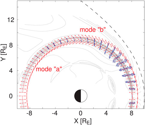
FIGURE 8. Reproduction of Figure 7 of Degeling et al. (2010). Grey contours: equatorial amplitude of E_α showing the FLR, taken 3 h after the start of the run, by which time the solution approximates a normal mode; blue vectors: equatorial electric field along the FLR peak, at various phases; red vectors: equatorial electric field polarization of the generalized SAW eigenfunctions (modes “a” and “b”) along their resonance surfaces (solid red lines); dashed line: the magnetopause boundary.

The discrepancy in the FLR location and polarization between the simulation and the unconstrained SAW eigenmodes of Kabin et al. (2007) is significant, indicating a constraint must be applied on the polarization of the SAW eigenmodes in order to correctly predict the FLR location. The results of Wright and Elsden (2016); Wright et al. (2018) demonstrate that the polarization direction in velocity perturbations should be aligned with contours of constant eigenfrequency. This effectively prevents the possibility of compressions or rarefactions in magnetic flux due to phase mixing, which is equivalent to requiring that the wave electric field for the SAW eigenmodes remains curl-free in order to remain compatible with the Alfvénic condition that b_γ = 0. An interesting feature of the red curves for modes “a” and “b” in Figure 8 is that they appear to correspond with the inner and outer L-shell boundaries of the FLR excited in the simulation. This may indicate that these red curves correspond with the inner and outer boundaries of the Resonant Zone of Wright and Elsden (2016) in a more general magnetic topology. For the dipole field equilibria in Section 2 these were identified through the requirement that the toroidal or poloidal ω_A equal the normal mode/driving frequency ω_d (Wright and Elsden, 2016). In more complex fields Wright et al. (2022) show this criterion need to be generalised to Max (ω_A) = ω_d and Min (ω_A) = ω_d. This suggests that the Alfvén eigenfunction calculation used to obtain Figure 7 corresponds to determining the modes with a special polarisation such that the maximum or minimum ω_A on the chosen field line matches the driving frequency. This contrasts with the solution to Eq. 8 where the polarisation is not constrained to correspond to the maximum or minimum ω_A, and suggests the Kabin et al. (2007) Alfvén eigenmodes may be used to determine the boundaries of the Resonant Zone, but cannot be used to generate the resonant paths within the Resonant Zone described by Eq. 7. The correspondence between Kabin’s Alfvén eigenmodes and the boundaries of the Resonant Zone is still to be established rigorously and warrants further investigation.

In order to more realistically model the coupling of SAWs with MHD fast mode waves launched by perturbations along the magnetopause boundary, the 3D MHD wave model of Degeling et al. (2010) was upgraded to incorporate the paraboloid magnetopause outer boundary of the Stern (1985) magnetic field model. In the new model (Degeling et al., 2018), Eqs. 11, 13 are solved using a finite element and a Galerkin spectral method respectively for the cross-field and field-aligned directions. Degeling et al. (2018) used the model to investigate the effect of a plasmaspheric density plume in the afternoon sector on the penetration of ULF wave power to the inner magnetosphere. The study demonstrated that the enhanced plasma density associated with the plume created a localized cavity in Alfvén speed, allowing the ducting, or trapping of fast mode waves that were able to penetrate deeply into the magnetosphere. This resulted in the strong excitation of FLRs at low L within the plume, with clear peaks associated with the fundamental mode resonance surfaces (calculated using the approach of Kabin et al. (2007)), and clear polarization shifts corresponding with changes in the local orientation of the surfaces. These effects are evident in Figure 9, which shows (in panels a–c) equatorial maps of the amplitude of radial and azimuthal electric field, as well as the field-aligned magnetic field. White dotted contours overlaid on these plots indicate the cold plasma density distribution, and resonant surface calculations are indicated by the magenta and dashed cyan lines.

FIGURE 9

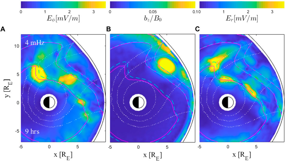
FIGURE 9. (A–C) (Reproduced from Degeling et al. (2018), Figures 2J–L): Equatorial amplitude maps of the ULF wave components E_ϕ, b_z/B₀ and E_r computed using the model of Degeling et al. (2018) for continuous externally driven 4 mHz waves along the dayside magnetopause boundary, under conditions where a plasmaspheric drainage plume has developed (over the preceding 9 h) in the afternoon sector. Magenta and dashed cyan lines in each plot indicate resonant surfaces calculated using the method of Kabin et al. (2007) for the fundamental, 3^rd and 5^th field-aligned harmonic eigenmodes; white dotted contours indicate cold plasma density (10,100 and 1,000 amu/cm³).

These results are consistent with the expectations from the 3-D Alfvén resonance theory of Wright and Elsden (2016) and the plume FLRs shown in Figure 6. Indeed, the strong deviations from axisymmetry in a plume makes it a prime location to find unambiguous observations of 3D FLRs. Elsden and Wright (2022) have shown the principal signature will be an Alfvén wave with both toroidal and poloidal fields, and there are already published case studies with these attributes that would be worth reinterpreting in terms of 3D FLRs (Clemmons et al., 2000; Hao et al., 2020; Le et al., 2021; Di Matteo et al., 2022). The Resonant Zone boundaries in Figure 9 suggested by the SAW eigenmode calculations are too narrow (and the model resolution is insufficient) to allow a detailed investigation of the role played by the magnetic topology in this scenario, indicating the need for a more detailed experiment.

A more specific investigation of the effect of changes in magnetic topology on the properties of the Resonant Zone using the 3-D MHD wave model of Degeling et al. (2018) has recently been carried out in Wright et al. (2022). In this work, the background magnetic field is provided by an “image dipole” vacuum magnetic field model, in which two dipole fields are summed together, with their axes separated by 30R_E and the strength of the second (image) dipole approximately 9.6 times the strength of the first, to give a compressed dipole field with subsolar magnetopause at x = 10R_E. A tailored equatorial density profile is used to provide a Resonant Zone with substantial width in L at high L-shell, where deviations in magnetic topology from a dipole field are more significant. The resulting Resonance Map for SAW normal modes with a specified driver frequency of 0.8 mHz is shown in Figure 10A. A clear asymptotic convergence of one class of Resonance Map trajectories is evident (marked by the green dashed line), starting at the inner boundary at local noon and moving smoothly to the outer boundary with MLT towards local midnight. According to Wright and Elsden (2016) this predicts the surface upon-which an FLR peak excited at the driver frequency with low m will have it is maximum amplitude. Near noon (midnight) MLT, Resonant Map trajectories are shown to approach the inner (outer) boundary of the Resonant Zone with near tangential polarization. The opposite is true for trajectories reaching the outer (inner) boundaries near noon (midnight) with near-perpendicular polarization. This is shown more clearly in 10(b), which shows the polarization angle (θ_r) as a function of MLT along the minimum (blue curve) and maximum (red curve) L-shell boundaries of the resonant zone. Note that θ_r is periodic over 180° because of the bi-directionality of the polarization. Interestingly, this corresponds very well with the polarization behavior of modes “a” and “b” shown in Figure 8 (with the polarization rotated through 90°, because electric field polarization used in Figure 8 is perpendicular to that of the velocity field used in Figure 10 under ideal MHD conditions).

FIGURE 10

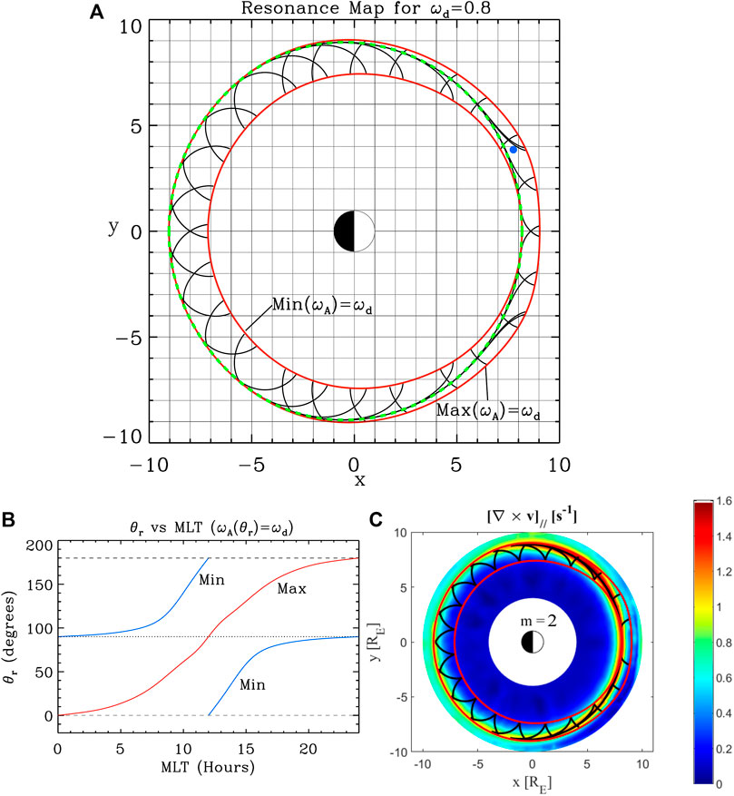
FIGURE 10. Summary of Resonant Zone investigations in a compressed dipole configuration (Taken from Wright et al. (2022), Figures 3A,B and Figure 4): (A) Calculation of Resonant Zone boundaries (solid red curves) and resonant paths (black curves) using the method of Wright and Elsden (2016). The green dashed line indicates the predicted peak location of a low m FLR; (B) Red (Blue) curves show the variation with MLT of equatorial polarization for the boundaries of the Resonant Zone corresponding to Max (ω_A) = ω_d (Min (ω_A) = ω_d); (C) Equatorial map of the parallel vorticity amplitude, |(∇ ×v)_‖|, (associated with SAWs) produced by the coupled MHD wave model of Degeling et al. (2018), for an externally driven 0.8 mHz wave source with m = 2 at the outer boundary. Solid black and red lines respectively indicate Resonance Map trajectories and Resonant Zone boundaries (using the same calculation method as plot (A).

The same density profile, magnetic field and driver frequency are used to calculate the coupled solutions to Eqs. 11, 13, using the 3D MHD wave model of Degeling et al. (2018). An equatorial map produced from the results, showing the amplitude of the field-aligned MHD flow vorticity |(∇ ×v)_‖| component for the case of a continuous outer boundary source with m = 2, is shown in Figure 10C. The narrow amplitude peak indicating the FLR location shows excellent agreement with the asymptote of converging trajectories in the Resonance Map (black lines overlaid in the plot), which proceeds smoothly from the inner boundary of the Resonant Zone at noon to the outer boundary at midnight (reproducing the behavior from Degeling et al. (2010) shown in Figure 8).

Figure 10 illustrates the utility of the Resonance Map in predicting the location of low m FLRs excited by an external MHD fast mode driver in compressed dipole magnetic field geometries. In situations where an asymptote of converging paths within the Resonant Zone exists and forms a closed surface, the FLR peak lies along this path, because essentially all paths within the Resonant Zone lead to the asymptote in this case (possibly after apparent reflections from the inner or outer boundaries). It is not clear, however, whether such an asymptote must exist in all cases, in which case it is important to consider whether the coupling from MHD fast modes to some paths at the Resonant Zone boundary is preferred over others.

As discussed in Section 2, in cases where the “azimuthal” derivatives of the equilibrium vanish, then the local polarization properties at the Resonant Zone boundary are reduced to 2D, and are strictly toroidal (poloidal), and tangential (normal) to the Resonant Zone boundary. Low m fast mode waves dominated by toroidal field line perturbations will most readily couple with the toroidal polarization at the symmetry axis of the Resonant Zone boundary, hence this selects the most strongly excited paths within the Resonant Zone. In more general configurations where no symmetry axis exists, it is shown in Wright et al. (2022) that a more general condition for optimum coupling between MHD fast mode waves and SAWs in the Resonant Zone is that the Resonant Zone boundary is locally tangential to the polarization at the boundary (referred to as the “tangential-alignment” criterion). This is demonstrated by a numerical experiment in Wright et al. (2022) in which an isolated local enhancement in cold plasma density in the afternoon sector is added to the density profile used to produce Figure 10, resulting in the equatorial Alfvén speed profile shown in Figure 11A. The Resonance Map (for waves with driver frequency 0.9 mHz in this case) is shown in Figure 11B. At this frequency the Resonant Zone is marked by a single boundary (the red solid line), which is localized in MLT to the afternoon sector. The resonance paths shown indicate that no line of asymptotic convergence (a separatrix) exists within the Resonant Zone in this case. Two blue points overlaid on the plot mark locations where the tangential-alignment criterion is satisfied (it could also be argued that these are points - rather than lines - of convergence of all resonance paths after multiple boundary reflections). Simulation results showing the absolute value of field-aligned vorticity in the equatorial plane are shown in Figure 11C, and demonstrate that the blue points in panel b correctly identify the location of strongest coupling, supporting the tangential-alignment criterion.

FIGURE 11

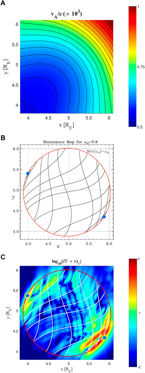
FIGURE 11. (Reproduced from Wright et al. (2022), Figure 5): (A): Equatorial Alfvén speed profile in the afternoon sector, showing an alteration due to the addition of a localized peak in density centered at (5, 5); (B): The Resonance Map in this case for a driver frequency of 0.9 mHz, showing a single closed boundary (red curve) and resonance paths from various boundary points (black curves). Blue points show locations on the boundary satisfying the tangential-alignment criterion (points along the Resonant Zone boundary where the mode polarization is tangential to the boundary); (C): Equatorial map of the parallel vorticity amplitude (log scale), showing peaks in amplitude that correspond well with the tangential-alignment condition (blue points). Also overlaid on the plot are the Resonant Zone boundary and resonance paths from panel b (red and white curves, respectively).

4 Analytical theory

This review is focused on the resonant coupling of fast waves to Alfvén waves. As shown in the previous sections, the simulation results tend to have a gentle ‘low-m’ variation with the FLRs forming a narrow ridge (aligned with the Alfvén wave plasma displacement) that can cross L-shells. Thus it may, at first sight, appear surprising that theoretical ideas developed for ‘high-m’ Alfvén waves have utility here. As explained in Elsden and Wright (2018), the common feature to both lines of study is that the Alfvén waves have a narrow transverse structure in the direction perpendicular to the background magnetic field and the Alfvén wave plasma displacement. To understand the development of related concepts developed elsewhere we divert briefly to high-m Alfvén waves.

4.1 High-m alfvén waves in 2-D

High-m Alfvén waves are termed ‘poloidal’ as the wave’s plasma displacement and field perturbation are confined to meridian planes and are perpendicular to B. These waves are normally thought to be excited by a resonant interaction with drifting ions (Southwood et al., 1969; Southwood and Kivelson, 1981, 1982). Leonovich and Mazur (1993) considered an alternative mechanism where extraneous ionospheric currents excited the waves. The equilibrium they considered was axisymmetric and similar to an axisymmetric dipole. To assist with interpreting their normal mode solution they constructed the diagram shown in Figure 12A, which is sketched in the equatorial plane. The outer circle represents the shell of field lines for which a toroidally polarised Alfvén wave (i.e. one with plasma displacement and perturbation field in the azimuthal direction) has a frequency matching that of the normal mode. It is termed the Toroidal surface or boundary.

FIGURE 12

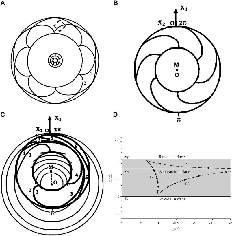
FIGURE 12. (A) shows the toroidal and poloidal boundaries (as circles) in the equatorial plane with two paths connecting them for an axisymmetric equilibrium (Leonovich and Mazur, 1993); (B) similar to (A) but only showing one set of paths between the boundaries; (C) shows the effect non-axisymmetry which makes system 3-D (Klimushkin et al., 1995); (D) a close up of the topology of paths and the separatrix surface in 3-D (Mager and Klimushkin, 2021).

Two sets of curved lines are shown in 12(a) that asymptote to the Toroidal boundary, and are labelled 1 and 2. These lines start at an inner circle where they are oriented perpendicular to the circle. The inner circle is termed the Poloidal surface or boundary, and is where the frequency of a poloidal Alfvén wave matches that of the normal mode. Leonovich and Mazur (1993) explain that the perpendicular group velocity of the Alfvén wave will cause it to change from having a poloidal polarisation (on the poloidal boundary) and move along the curved paths (1 or 2) to the toroidal boundary. As the wave travels its polarisation rotates smoothly such that its local k_⊥ is normal to the curved path. The authors used the term ‘transparency region’ to describe the region containing these paths. The scenario described above may appear to have some surprising properties. For example, Alfvén waves are renowned for having a field-aligned group velocity and their energy staying on one field line–so how can they travel across field lines?

There is certainly evidence from the time dependent simulations of Mann and Wright (1995) that an initially poloidal Alfvén wave will phasemix and have its polarisation rotate to toroidal. However, their study used a uniform magnetic field meaning the toroidal and poloidal frequencies on a given field line are identical–i.e., the toroidal and poloidal boundaries coincide. Thus, this work did not require the Alfvén wave to follow a path that crossed field lines. Sarris et al. (2009) have also reported observational evidence for the change of polarisation.

A more recent study by Elsden and Wright (2020) used a 2-D dipole field for which the poloidal and toroidal surfaces are well separated and form the boundaries of the Resonant Zone as described in the Resonance Map formulation of Figure 3. The time-dependent results of this study showed that as high-m poloidal Alfvén waves evolve they do indeed follow the paths in the Resonant Zone as they phasemix and turn towards a toroidal polarisation. Indeed the transparency region of Leonovich and Mazur (1993) and the Resonant Zone of Wright and Elsden (2016), and the paths therein are the same construction. It is interesting that the paths were derived by Leonovich and Mazur (1993) as contours of an asymptotic phase that initially poloidal Alfvén waves would move along. In contrast Wright and Elsden (2016) were looking at low-m resonant Alfvén waves excited by the fast mode. Their simulations led to the formulation of the Resonance Map based on the recognition that the Alfvén frequency depends on the wave’s polarisation angle (which is aligned with the plasma displacement) and is tangential to the resonant paths. Thus we have two complementary and independent ways of deriving the resonant paths within the Resonant Zone/Transparency Region.

Whilst the asymptotically narrow nature of the Alfvén wave solutions is explicity stated in the formulation of Leonovich and Mazur (1993), it is also implicit in the description of Wright and Elsden (2016): their generalisation of the Alfvén wave equation (Singer et al., 1981, their Equation 9) to an arbitrary polarisation required the width across the resonance be much less than the scale length along the resonant path. There were also related orderings that the size of the Alfvén wave’s magnetic and velocity fields along these paths be much greater than the components perpendicular to the path. There is also an even smaller compressional magnetic field. In this sense these Alfvén waves are not a decoupled free oscillation in the way that an axisymmetric m = 0 toroidal Alfvén wave is. However it is valid to say that a 3-D Alfvén wave can be regarded as an ‘asymptotically’ decoupled free mode.

The presence of asymptotically small fields perpendicular to the resonant paths (and also a small compressional field) can account for the fact that the group velocity and energy flow is no longer strictly field aligned. Indeed Elsden and Wright (2020) explain how the process operates in a time-dependent setting: the leading Alfvén wave fields produce an asymptotically small magnetic pressure that oscillates with the same frequency as the main Alfvén wave. This creates a pressure gradient that will act on all the surrounding plasma and can potentially excite waves on these field lines (Elsden and Wright, 2017). There is one neighbouring field line that will respond particularly efficiently to such a pressure gradient–it is the field line a small distance down the resonant path. The Alfvén wave on this field line with plasma displacement tangential to the path will have a resonant response to the magnetic pressure driver. Other field lines will have a non-resonant response. In this fashion the Alfvén wave can travel along the resonant paths, as predicted by Leonovich and Mazur (1993).

4.2 High-m alfvén waves in 3-D

The behaviour of high-m poloidal Alfvén waves was generalised to 3-D by Klimushkin et al. (1995). Figure 12B shows the axisymmetric 2-D case and is similar to panel (a) except that only one set of the resonant paths is shown. The equilibrium is made 3-D by retaining the axisymmetric magnetic field, but allowing the density to vary with all three coordinates. The resulting Resonance Map is shown in 12(c), again for just one set of the resonant paths. The boundaries of the Resonant Zone are still the toroidal and poloidal boundaries and the density is chosen so that these are still concentric circles, however they are no longer centered on the magnetic axis (O).

The inner bold circle in Figure 12C (the poloidal boundary) has paths connecting to it that are aligned with the radial direction (i.e., directed away from O). There are paths (like those labelled 1 and 2) that connect the inner (poloidal) boundary to the outer (toroidal) boundary, where they adopt an azimuthal alignment. However there is now a new class of paths (like 6) that start and finish on the toroidal boundary. The two topologically distinct regions are defined by a separatrix as described by Klimushkin et al. (1995) and Mager and Klimushkin (2021). Figure 12D is taken from the latter paper and is a close up of a section of the Resonant Zone. The local coordinates x and y are based on the poloidal and toroidal boundaries. Note that these boundaries are not aligned with the radial or azimuthal directions. The radial direction can be inferred from the alignment of the resonant paths connecting to the poloidal boundary. Similarly the azimuthal direction aligns with the paths as they connect to the toroidal boundary. Whilst one set of paths can cross from the poloidal to the toroidal boundary, there are now two other types of paths. They are connected to either the toroidal or poloidal boundary and then asymptote to the separatrix. This behaviour is seen very clearly in Figure 3B.

4.3 Field line resonances in 3-D

More recently the study of Mager and Klimushkin (2021) has considered asymptotic solutions of FLRs. However, their formulation is still for the high-m limit, which means the fast mode is evanescent and so neglected from their solutions. Therefore, they are still focusing on Alfvénic normal modes, which they describe in terms of travelling along the resonant paths shown in Figure 12D. They note that the Alfvén wave energy will accumulate at the separatrix surface as the wave energy travels along the resonant paths which converge towards the separatrix. Thus they identified the resonant surface as coinciding with the separatrix.

In the classic 1-D FLR of Southwood (1974) the solution has a singularity where the azimuthal velocity and magnetic field of the Alfvén wave vary as ${(x-x_r)}^{-1}$, where ω_A (x_r) matches the normal mode frequency. The radial components are also infinite at x_r, but vary as ln (x − x_r). These properties are also present in FLRs in 2-D axisymmetric equilibria (Wright and Thompson, 1994). It is interesting that the 3-D FLR solutions of Mager and Klimushkin (2021) retain the simple pole singularity in the velocity and magnetic fields tangential to the resonant path, but the logarithmic singularity in the components normal to the path is no longer present. Indeed they find that these fields remain finite as the resonant surface is approached and undergo increasingly rapid spatial oscillations. This behaviour is quite different to simpler models of FLRs and worthy of further investigation.

Mager and Klimushkin (2021) also derived the solutions of resonant Alfvén waves along the resonant paths as they approach the boundaries of the Resonant Zone. They found that the solution took the form of an Airy Function: it had a propagating (oscillatory) nature within the Resonant Zone which turned to an exponentially decaying form on crossing the boundary to the Non-Resonant Zone. This is qualitatively supported by the simulations shown in Figure 3A. It is evident that as the resonant ridge in the lower right corner approaches the left-hand boundary (shown as a red line) it becomes evanescent on crossing the boundary. This is physically reasonable behaviour since the field lines to the left of the boundary will be non-resonant. Moreover, the further a field line is from the Resonant Zone boundary the larger the discrepancy between its Alfvén frequency and that of the normal mode–hence the smaller the Alfvén waves established there. Thus we anticipate a non-resonant response on these field lines, which is consistent with the rapid fall in amplitude. This behaviour is also reminiscent of quantum mechanical tunnelling.

An alternative analytical formulation is presented by Cheng (2003) for a plasma having nonzero pressure and equilibrium current. The formulation uses Euler potentials ψ and α_c as transverse coordinates, B = ∇ψ ×∇α_c. The radial-like coordinate ψ is the flux function and α_c an azimuthal-like coordinate. (We have added a subscript ‘c’ to avoid confusion with the use of α in previous sections.) The modelling described in solved for the components of the wave fields projected onto the coordinate directions, which may have orthogonal or non-orthogonal unit vectors. Cheng (2003) sidesteps this issue by constructing local orthogonal directions by using the vectors B and ∇ψ to form B ×∇ψ and complete the orthogonal basis (see Figure 13A). Cheng expresses the plasma displacement in the B ×∇ψ direction in terms of the quantity ξ_s which represents the Alfvén wave.

FIGURE 13

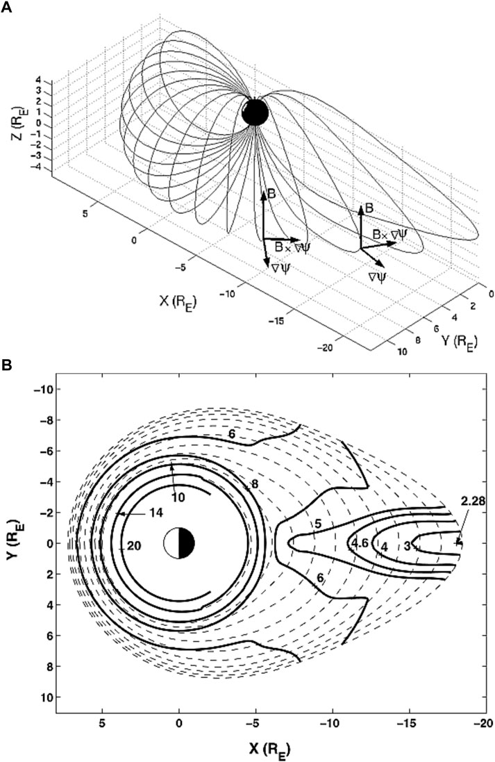
FIGURE 13. (A) The model field and directions of the unit vectors used by Cheng (2003); (B) a view in the equatorial plane of ψ contours (dashed lines) and contours of ω_A (solid lines) for Alfvén waves polarised with plasma displacement tangential to the dashed lines.

Figure 13B shows contours of ψ in the equatorial plane as dashed lines. Cheng (2003) explains how the natural Alfvén frequencies may be calculated in the equatorial plane. It is noteworthy, in light of the importance of wave polarisation stressed throughout this review, that these frequencies correspond to Alfvén waves with plasma displacement tangential to the dashed lines in Figure 13B. For these polarisations, ω_A (ψ, α_c) may be determined and contours of this frequency are shown as the solid lines in Figure 13B.

In general contours of ω_A (ψ, α_c) and ψ do not coincide. Cheng suggests that the line ω_A (ψ, α_c) = ω_d will be the resonant Alfvén wave surface when driven with frequency ω_d, and to facilitate the analysis further introduces new coordinates (which we denote by ψ₁ and α_c1) such that the contour ψ₁ = ψ₀ labels the resonant field line surface, i.e., ω_A (ψ₁ = ψ₀, α_c1) = ω_d. For example, if we were interested in the case for ω_d = 6, then the line ψ₁ = ψ₀ coincides with the solid black line Figure 13B with value 6. It is not obvious that this will be the resonant surface as evaluating ω_A (ψ₁ = ψ₀, α_c1) will be the frequency of an Alfvén wave with displacement tangential to the ψ₁ contours–i.e., the solid black lines. This will be a different Alfvén wave to that calculated with the original ψ, which had displacement tangential to the dashed lines. As the polarisation has changed so will ω_A. This means black lines will not be contours of ω_A for Alfvén waves with displacement tangential to these lines. It may be possible to iterate this process to converge on a suitable solution.

For resonant Alfvén waves, what is needed is a path in the equatorial plane such that when ω_A is calculated for an Alfvén wave with displacement tangential to the path we find ω_A = ω_d. These are the very paths described by Wright and Elsden (2016) and examples of these paths are shown in Figures 3, 4, 12. Note that these figures show a Resonant Zone with an infinite number of possible resonant paths for a given driving frequency, in contrast to Figure 13 which shows a single line for a given frequency. Cheng (2003) goes on to derive the nature of the singularity along a resonant path and finds the ξ_s Alfvén field (aligned with B ×∇ψ₁) scales as 1/(ψ₁ − ψ₀) and the displacement normal to the resonant path (aligned with ∇ψ₁) scales as ln (ψ₁ − ψ₀). These properties are in accord with the results in 1-D (e.g., Southwood (1974)) and 2-D (e.g., Wright and Thompson (1994) and Russell and Wright (2010)), but contrary to the 3-D results of Mager and Klimushkin (2021) who claim the logarithmic singularity is removed in a 3-D system.

A final analytical study addressing 3D FLRs was undertaken by Inhester (1986) and took an alternative approach by identifying FLRs as field lines where the Poynting vector indicated the resonant absorption of energy. Whilst the 1-D and 2-D limits of Inhester’s formulation are in accord with the relevant literature, it identifies unusual features when applied to a 3-D equilibrium. The paper notes that a lack of axisymmetry in 3-D will cause a conflict with the requirement that the FLR be (essentially) incompressible, and this will prevent resonant absorption occuring. Inhester goes on to estimate, for realistic magnetospheric parameters, that fundamental FLRs whose polarisation deviates by more than 14° from toroidal will be suppressed. This claim is contradictory to the simulation results in Figure 6 which shows an FLR polarisation on the edge of a plume turning though around 60° yet still undergoing strong resonant excitation.

5 Discussion and conclusion

In this section, we briefly summarise the results presented in the three main sections above for ease of reference. We also discuss the implications of 3-D FLRs in terms of observations and wave-particle interactions, as well as highlighting current unknowns and areas of contention which require further research.

5.1 Simulations

Given the difficulty of finding analytical solutions to the full 3-D Alfvén resonance problem (as highlighted in the next subsection), numerical simulations have proven to be a critical tool in furthering our understanding of this phenomena. The ‘simpler’ simulations presented in section 2 based on 2-D and 3-D magnetic dipole geometries, have shown great utility in providing fundamental new answers regarding 3-D FLRs. This review has summarised:

• Simulations showing the resonant excitation of intermediate polarisation (between poloidal and toroidal) Alfvén waves in a 3-D non-uniform plasma.

• How to calculate the Alfvén frequency for a mode of such intermediate polarisation (see Eq. 6).

• Where FLRs form in 3-D - introduction of the Resonance Map (Figure 3B) to depict mathematically permissible solutions.

• Extension of established theories in 1-D/2-D to 3-D e.g. estimates of time-dependent resonance widths and amplitudes, and the requirement of a fast mode magnetic pressure gradient tangential to the resonance.

• The potential utility of the solutions of Kabin et al. (2007) in directly determining Resonance Map boundaries and the boundary polarization in 3-D magnetic fields (an area of continuing study).

There are several problems to which these simulations can be applied in future studies. To fully understand where FLRs will form and how efficient the fast-Alfvén wave coupling will be, the spatial and temporal structure of the global fast waves must be determined. Previous simulation studies have considered how the fast mode will behave in a 3-D non-uniform magnetosphere (Degeling et al., 2018; Wright et al., 2018; Elsden and Wright, 2019; Wright and Elsden, 2020). These works show that the inclusion of such non-uniformity (e.g., through a plasmaspheric drainage plume on the dusk flank) act to create significant spatial structure in the fast mode. For example, the enhanced density cavity of a plume can itself support local cavity modes (Degeling et al., 2018). These could contribute significantly to the excitation of 3-D FLRs within the plume. Azimuthal gradients in the plasma density further cause refraction of the fast mode, affecting where sufficient gradients in the fast mode exist to effectively drive FLRs (Wright et al., 2018). More simulations of these features are certainly required to better understand the full picture of 3-D magnetospheric fast-Alfvén wave coupling.

5.2 Analytical theory

Key properties of the resonant paths and Resonance Maps that are central to understanding 3-D FLRs were first applied to high-m poloidal Alfvén waves driven by extraneous ionospheric currents (Leonovich and Mazur, 1993; Klimushkin et al., 1995). These authors showed how poloidal Alfvén waves could drift across field lines and change their polarisation. The simulations of Elsden and Wright (2020) show this is possible because the poloidal waves are not pure decoupled Alfvén waves, but “asymptotically decoupled” Alfvén waves. Leonovich and Mazur (1993) give formulae for the speed with which the waves travel along the resonant paths, and it would be useful to demonstrate the use of these expressions through interpreting simulation results.

Developing analytical theory for 3-D FLRs is a considerable challenge and generally requires some simplifying assumptions. For example, Mager and Klimushkin (2021) seek solutions with a large azimuthal wavenumber, and note this means the fast mode is evanescent and may be neglected. This may cause some to question whether their solution corresponds to an Alfvén wave that is driven resonantly by a fast mode as in the normal picture of an FLR.

The simulations of 3-D FLRs reviewed in the previous sections show that FLRs are narrow (and so, in some sense, are ‘high-m’) but also have a large radial-like wavenumber. In contrast, the fast mode driving the FLRs is not a high-m wave. Generally we do not expect a low-m fast mode to couple effectively to a high-m FLR. However, the variation of FLR properties along special paths (the resonant paths) does not have a high wavenumber, but a gentle variation over large scales. Indeed, in the formulation of Mager and Klimushkin (2021) the resonant paths are contours of their WKB phase. Moreover Elsden and Wright (2017) have shown how the gradient of the fast mode magnetic pressure resolved along the resonant paths is responsible for driving the FLR response. Motivated by the simulations, it would be worth investigating the possibility of combining these ideas to generate an analytical solution where a low-m fast mode is used to drive an Alfvén wave response that is narrow perpendicular to the resonant path, but has a gentle variation along it.

The analytical solution of Mager and Klimushkin (2021) stress the importance of the separatrix in the Resonance Map and claim that of all the possible resonant paths it is the one coinciding with the separatrix where the resonant FLR is excited. It is true that the separatrix is a special path and resonant paths converge to it, meaning that it is likely to have substantial Alfvén wave energy on or near it in certain places. However, it is also possible for other resonant paths to carry the main FLR. Wright and Elsden (2016) show that if the Resonant Zone intersects a simulation boundary, then the boundary conditions there will determine which resonant path the FLR is on. In general this is different to the separatrix path. Of course, as the FLR resonant path is traced away from the boundary it may converge to the separatrix and for practical purposes be indistinguishable from it in some locations.

It would be desirable to have a more detailed understanding of identifying which resonant paths the FLRs coincide with. No doubt identifying the separatrix and locations where the “tangential alignment” condition is met will be key ingredients. However, other resonant paths can support FLRs through other processes. For example, in Figure 4A the FLR produced at the strong coupling location at (0.9,0) zig-zags as it bounces between encounters with the boundary of the Resonant Zone, where it switches to resonant paths that do not satisfy either the “separatrix” or “tangential alignment” conditions. The nature of the interaction of an FLR with the Resonant Zone boundaries is not understood well and warrants further investigation.

The formulation of Cheng (2003) is closer to the singular series solution of FLRs used in 1-D and 2-D (e.g., Southwood (1974) and Wright and Thompson (1994)) than the asymptotic theory of Mager and Klimushkin (2021). However, the new feature in 3-D of the Resonant Zone containing a continuum of possible resonant paths is not considered by Cheng (2003) – as evidenced by a single driving frequency corresponding to a single resonant path in Figure 13B rather than a Resonant Zone. Although there are questions concerning how Cheng (2003) determines the path of the FLR (see ), there is much merit in the paper. For example, if the resonant path was determined by using Eq. 7 and simulations, then this path could be used to define Cheng’s transverse coordinates and we can benefit from their subsequent analysis. In particular, Cheng (2003) finds that the transverse fields have the usual single pole and logarithmic singularities familiar from the 1-D and 2-D limits. Interestingly, Mager and Klimushkin (2021) claim the logarithmic singularity is not present in 3-D, and whilst there is a jump in amplitude on crossing the FLR, the amplitude remains finite. It is likely that simulations can be used to confirm the true nature of the singularity. Indeed, developing the challenging theory of 3-D FLRs has taken substantial steps when simulations are used to guide the development of theory, and this approach will likely prove efficacious in future studies.

5.3 Implications of 3-D field line resonances

In the final part of this review, we would like to discuss (and leave open for readers to think about) what we believe are/could be the key implications from the 3-D aspect of FLRs. It is of course important to understand this process from a pure physics standpoint, but there are also several areas of immediate application in the magnetosphere.

Firstly let us treat the potential observation of 3-D FLRs. With the recent developments in the theory of 3-D FLRs, it has now become possible to identify clear features which should be visible in spacecraft and ground-based data. Elsden and Wright (2022) present simulations which analyse what a satellite would observe passing through a 3-D FLR. Very evident is the contribution of the FLR to both radial and azimuthal components of the fields. When the FLR amplitude is sufficiently greater than that of the fast mode (which can be checked by confirming an appropriately small parallel magnetic field component near the equatorial plane), the following features should identify a 3-D FLR:

• Local amplitude increase (same as classical FLR criteria).

• Radial and azimuthal field components (magnetic, velocity or electric) will be in/out of phase. This will result in an approximately linear hodogram.

• The systematic variation of FLR polarisation angle with azimuth (MLT) across the density gradients present in a plasmaspheric plume should be identifiable in ground magnetometer and satellite data.

The 3-D nature of FLRs should also affect the spatial structure of the FLR driven aurora. A toroidal FLR can generate poleward moving auroral arcs (Milan et al., 2001; Rankin et al., 2005; Gillies et al., 2018), with the excitation occurring about a central latitude corresponding to the central field line of the FLR in space. For a 3-D FLR, one would expect to see an auroral arc crossing magnetic latitude, which can be pictured as the ground footprint of the curved FLR which crosses L-shells shown in Figure 6B.

The predominant interest in ULF wave research in recent years has been their influence on particles in the Earth’s radiation belts. Since the periods of ULF waves can coincide with the drift period of energetic particles in the radiation belts, there can exist a drift-resonant interaction between the waves and particles (Southwood and Kivelson, 1981). When considering multiple ULF waves across a range of frequencies, the interaction leads to the radial diffusion of particles, violating the third adiabatic invariant. Assuming that the first adiabatic invariant associated with particle gyromotion is conserved, this also results in a change in the particle energies (Fälthammar, 1965; Elkington et al., 2003).

Of interest for this review is the effect that mixed polarisation FLRs could have on particle energisation. Elkington et al. (2003)reports on the effect of poloidal and toroidal mode ULF waves on particles, showing that when included in a compressed dipole magnetic field model with a convection electric field, both modes can contribute significantly to particle energisation. It would therefore be expected that modes of intermediate polarisation should also have an effect. Indeed, Ozeke et al. (2012) invoke exactly this explanation when calculating the electric field diffusion coefficient. They consider that in a symmetric dipole magnetic field, only the azimuthal component of the electric field (parallel to the electron drift direction) associated with the FLR should be used in the diffusion coefficient calculation. This would correspond to a poloidal mode, but interestingly the authors argue that such a poloidal component could be contributed by a mixed polarisation FLR, as observed by Clemmons et al. (2000) and analysed as an FLR by Ozeke et al. (2005). The framework of 3-D FLRs lends credence to this idea, and it would therefore be expected that the contribution to the azimuthal electric field component from 3-D FLRs should be important in this context. The highly localized radial structure of narrow band FLRs may be expected to have a limited impact on radial transport, however Degeling et al. (2019) has shown that alterations in drift resonance dynamics due to strongly peaked FLRs act to extend the L-shell range of the interaction. The radial span of the resonant zone for 3-D FLRs in compressed dipole geometries potentially provides a further extension in their effective range in L-shell. Further investigation into these effects using test-particle simulations like those of Elkington et al. (2003); Hudson et al. (2017); Degeling et al. (2007); Degeling and Rankin (2008); Degeling et al. (2014) using mixed polarisation ULF waves should be addressed in future studies.

Author contributions

All authors listed have made a substantial, direct, and intellectual contribution to the work and approved it for publication.

Funding

TE is funded by a Leverhulme Trust Early Career Fellowship (ECF-2019–155) and the University of Glasgow. AW was partially funded by the Science and Technology Facilities Council (STFC) grant (ST/N000609/1). AD is supported by the National Natural Science Foundation of China (41,774,172).

Acknowledgments

This review was written as part of the activities of an international team whose workshops were sponsored by the International Space Science Institute (ISSI) in Bern, Switzerland. The authors are all members of this team and are grateful to ISSI for their support. AW, AD gratefully acknowledges many collaborative discussions with R. Rankin and the use of computing facilities at University of Alberta during this work.

Conflict of interest

The authors declare that the research was conducted in the absence of any commercial or financial relationships that could be construed as a potential conflict of interest.

Publisher’s note

All claims expressed in this article are solely those of the authors and do not necessarily represent those of their affiliated organizations, or those of the publisher, the editors and the reviewers. Any product that may be evaluated in this article, or claim that may be made by its manufacturer, is not guaranteed or endorsed by the publisher.

References

Alfvén, H. (1942). Existence of electromagnetic-hydrodynamic waves. Nature 150, 405–406. doi:10.1038/150405d0

CrossRef Full Text | Google Scholar

Allan, W., and Knox, F. B. (1979). A dipole field model for axisymmetric alfvén waves with finite ionosphere conductivities. Planet. Space Sci. 27, 79–85. doi:10.1016/0032-0633(79)90149-1

CrossRef Full Text | Google Scholar

Allan, W., Poulter, E. M., and White, S. P. (1986a). Hydromagnetic wave coupling in the magnetosphere - plasmapause effects on impulse-excited resonances. Planet. Space Sci. 34, 1189–1200. doi:10.1016/0032-0633(86)90056-5

CrossRef Full Text | Google Scholar

Allan, W., White, S. P., and Poulter, E. M. (1986b). Impulse-excited hydromagnetic cavity and field-line resonances in the magnetosphere. Planet. Space Sci. 34, 371–385. doi:10.1016/0032-0633(86)90144-3

CrossRef Full Text | Google Scholar

Allan, W., White, S. P., and Poulter, E. M. (1985). Magnetospheric coupling of hydromagnetic waves - initial results. Geophys. Res. Lett. 12, 287–290. doi:10.1029/GL012i005p00287

CrossRef Full Text | Google Scholar

Burghes, D. N., Kendall, P. C., and Sweet, P. A. (1969). A Physical explanation of difficulties appearing in the theory of toroidal magnetohydrodynamic oscillations. Mon. Notices R. Astronomical Soc. 143, 9–16. doi:10.1093/mnras/143.1.9

CrossRef Full Text | Google Scholar

Chen, L., and Cowley, S. C. (1989). On field line resonances of hydromagnetic Alfven waves in dipole magnetic field. Geophys. Res. Lett. 16, 895–897. doi:10.1029/GL016i008p00895

CrossRef Full Text | Google Scholar

Chen, L., and Hasegawa, A. (1974). A theory of long-period magnetic pulsations: 1. Steady state excitation of field line resonance. J. Geophys. Res. 79, 1024–1032. doi:10.1029/JA079i007p01024

CrossRef Full Text | Google Scholar

Cheng, C. Z., Chang, T. C., Lin, C. A., and Tsai, W. H. (1993). Magnetohydrodynamic theory of field line resonances in the magnetosphere. J. Geophys. Res. 98, 11339–11348. doi:10.1029/93JA00505

CrossRef Full Text | Google Scholar

Cheng, C. Z. (2003). MHD field line resonances and global modes in three-dimensional magnetic fields. J. Geophys. Res. 108, 1002. doi:10.1029/2002JA009470

CrossRef Full Text | Google Scholar

Cheng, C. Z., and Zaharia, S. (2003). Field line resonances in quiet and disturbed time three-dimensional magnetospheres. J. Geophys. Res. 108, 1001. doi:10.1029/2002JA009471

CrossRef Full Text | Google Scholar

Claudepierre, S. G., Mann, I. R., Takahashi, K., Fennell, J. F., Hudson, M. K., Blake, J. B., et al. (2013). Van Allen Probes observation of localized drift resonance between poloidal mode ultra-low frequency waves and 60 keV electrons. Geophys. Res. Lett. 40, 4491–4497. doi:10.1002/grl.50901

CrossRef Full Text | Google Scholar

Clemmons, J. H., Pfaff, R. F., Lennartsson, O. W., Mozer, F. S., Singer, H. J., Peterson, W. K., et al. (2000). Observations of traveling Pc5 waves and their relation to the magnetic cloud event of January 1997. J. Geophys. Res. 105, 5441–5452. doi:10.1029/1999JA900418

CrossRef Full Text | Google Scholar

Cummings, W. D., O’Sullivan, R. J., and Coleman, J. (1969). Standing Alfvén waves in the magnetosphere. J. Geophys. Res. 74, 778–793. doi:10.1029/JA074i003p00778

CrossRef Full Text | Google Scholar

Degeling, A. W., Rae, I. J., Watt, C. E. J., Shi, Q. Q., Rankin, R., and Zong, Q. G. (2018). Control of ULF wave accessibility to the inner magnetosphere by the convection of plasma density. J. Geophys. Res. Space Phys. 123, 1086–1099. doi:10.1002/2017JA024874

CrossRef Full Text | Google Scholar

Degeling, A. W., Rankin, R., Kabin, K., Marchand, R., and Mann, I. R. (2007). The effect of ULF compressional modes and field line resonances on relativistic electron dynamics. Planet. Space Sci. 55, 731–742. doi:10.1016/j.pss.2006.04.039

CrossRef Full Text | Google Scholar

Degeling, A. W., Rankin, R., Kabin, K., Rae, I. J., and Fenrich, F. R. (2010). Modeling ULF waves in a compressed dipole magnetic field. J. Geophys. Res. 115, A10212. doi:10.1029/2010JA015410

CrossRef Full Text | Google Scholar

Degeling, A. W., and Rankin, R. (2008). Resonant drift echoes in electron phase space density produced by dayside pc5 waves following a geomagnetic storm. J. Geophys. Res. 113. doi:10.1029/2008JA013254

CrossRef Full Text | Google Scholar

Degeling, A. W., Rankin, R., Wang, Y., Shi, Q. Q., and Zong, Q.-G. (2019). Alteration of particle drift resonance dynamics near poloidal mode field line resonance structures. J. Geophys. Res. Space Phys. 124, 7385–7401. doi:10.1029/2019JA026946

CrossRef Full Text | Google Scholar

Degeling, A. W., Rankin, R., and Zong, Q.-G. (2014). Modeling radiation belt electron acceleration by ulf fast mode waves, launched by solar wind dynamic pressure fluctuations. J. Geophys. Res. Space Phys. 119, 8916–8928. doi:10.1002/2013JA019672

CrossRef Full Text | Google Scholar

D’haeseleer, W. D., Hitchon, W. N. G., Callen, J. D., and Shohet, J. L. (1991). Flux coordinates and magnetic field structure. Berlin, Germany: Springer-Verlag. doi:10.1007/978-3-642-75595-8

CrossRef Full Text | Google Scholar

Di Matteo, S., Villante, U., Viall, N., Kepko, L., and Wallace, S. (2022). On differentiating multiple types of ulf magnetospheric waves in response to solar wind periodic density structures. J. Geophys. Res. Space Phys. 127, e2021JA030144. doi:10.1029/2021JA030144

PubMed Abstract | CrossRef Full Text | Google Scholar

Dungey, J. W. (1955). Electrodynamics of the outer atmosphere. Phys. Ionos. 229.

Google Scholar

Dungey, J. W. (1954). Electrodynamics of the outer atmosphere: Report to national science foundation on work carried on under grant NSF-G450. Scientific report//ionospheric research, ionosphere research labor. Pennsylvania: The Pennsylvania State University (Pennsylvania State University, Ionosphere Research Laboratory).

Google Scholar

Elkington, S. R., Hudson, M. K., and Chan, A. A. (1999). Acceleration of relativistic electrons via drift-resonant interaction with toroidal-mode Pc-5 ULF oscillations. Geophys. Res. Lett. 26, 3273–3276. doi:10.1029/1999GL003659

CrossRef Full Text | Google Scholar

Elkington, S. R., Hudson, M. K., and Chan, A. A. (2003). Resonant acceleration and diffusion of outer zone electrons in an asymmetric geomagnetic field. J. Geophys. Res. 108, 1116. doi:10.1029/2001JA009202

CrossRef Full Text | Google Scholar

Elsden, T. (2016). Numerical modelling of ultra low frequency waves in Earth’s magnetosphere. Ph.D. thesis. St. Andrews: University of St. Andrews. Availableat: http://hdl.handle.net/10023/15663.

Google Scholar

Elsden, T., and Wright, A. N. (2020). Evolution of high-m poloidal alfvén waves in a dipole magnetic field. J. Geophys. Res. Space Phys. 125, e28187. doi:10.1029/2020JA028187

CrossRef Full Text | Google Scholar

Elsden, T., and Wright, A. N. (2022). Polarization properties of 3-D field line resonances. JGR. Space Phys. 127, e30080. doi:10.1029/2021JA030080

CrossRef Full Text | Google Scholar

Elsden, T., and Wright, A. N. (2018). The broadband excitation of 3-D alfvén resonances in a MHD waveguide. JGR. Space Phys. 123, 530–547. doi:10.1002/2017JA025018

CrossRef Full Text | Google Scholar

Elsden, T., and Wright, A. N. (2019). The effect of fast normal mode structure and magnetopause forcing on FLRs in a 3-D waveguide. J. Geophys. Res. Space Phys. 124, 178–196. doi:10.1029/2018JA026222

CrossRef Full Text | Google Scholar

Elsden, T., and Wright, A. N. (2017). The theoretical foundation of 3-D Alfvén resonances: Time-dependent solutions. J. Geophys. Res. Space Phys. 122, 3247–3261. doi:10.1002/2016JA023811

CrossRef Full Text | Google Scholar

Fälthammar, C.-G. (1965). Effects of time-dependent electric fields on geomagnetically trapped radiation. J. Geophys. Res. 70, 2503–2516. doi:10.1029/JZ070i011p02503

CrossRef Full Text | Google Scholar

Gillies, D. M., Knudsen, D., Rankin, R., Milan, S., and Donovan, E. (2018). A statistical survey of the 630.0-nm optical signature of periodic auroral arcs resulting from magnetospheric field line resonances. Geophys. Res. Lett. 45, 4648–4655. doi:10.1029/2018GL077491

CrossRef Full Text | Google Scholar

Goldstein, J., Sandel, B. R., Forrester, W. T., Thomsen, M. F., and Hairston, M. R. (2005). Global plasmasphere evolution 22-23 April 2001. J. Geophys. Res. 110, A12218. doi:10.1029/2005JA011282

CrossRef Full Text | Google Scholar

Hao, Y. X., Zhao, X. X., Zong, Q.-G., Zhou, X.-Z., Rankin, R., Chen, X. R., et al. (2020). Simultaneous observations of localized and global drift resonance. Geophys. Res. Lett. 47. doi:10.1029/2020GL088019

CrossRef Full Text | Google Scholar

Heyvaerts, J., and Priest, E. R. (1983). Coronal heating by phase-mixed shear Alfven waves. Astronomy Astrophysics 117, 220–234.

Google Scholar

Hudson, M., Jaynes, A., Kress, B., Li, Z., Patel, M., Shen, X.-C., et al. (2017). Simulated prompt acceleration of multi-mev electrons by the 17 march 2015 interplanetary shock. J. Geophys. Res. Space Phys. 122 (10), 10036–10046. doi:10.1002/2017JA024445

CrossRef Full Text | Google Scholar

Hughes, W. J. (1994). Magnetospheric ULF waves: A tutorial with a historical perspective. Wash. D.C. Am. Geophys. Union Geophys. Monogr. Ser. 81, 1–11. doi:10.1029/GM081p0001

CrossRef Full Text | Google Scholar

Inhester, B. (1987). Numerical modeling of hydromagnetic wave coupling in the magnetosphere. J. Geophys. Res. 92, 4751–4756. doi:10.1029/JA092iA05p04751

CrossRef Full Text | Google Scholar

Inhester, B. (1986). Resonance absorption of Alfvén oscillations in a nonaxisymmetric magnetosphere. J. Geophys. Res. 91, 1509–1518. doi:10.1029/JA091iA02p01509

CrossRef Full Text | Google Scholar

Kabin, K., Rankin, R., Mann, I. R., Degeling, A. W., and Elkington, S. R. (2009). “Polarization properties of the ultra-low frequency waves in non-axisymmetric background magnetic fields,” in Advances in geosciences (World Scientific Publishing Company), 14, 225–235. doi:10.1142/9789812836205_0016

CrossRef Full Text | Google Scholar

Kabin, K., Rankin, R., Mann, I. R., Degeling, A. W., and Marchand, R. (2007). Polarization properties of standing shear Alfvén waves in non-axisymmetric background magnetic fields. Ann. Geophys. 25, 815–822. doi:10.5194/angeo-25-815-2007

CrossRef Full Text | Google Scholar

Kageyama, A., Sugiyama, T., Watanabe, K., and Sato, T. (2006). A note on the dipole coordinates. Comput. Geosci. 32, 265–269. doi:10.1016/j.cageo.2005.06.006

CrossRef Full Text | Google Scholar

Kivelson, M. G., and Southwood, D. J. (1986). Coupling of global magnetospheric MHD eigenmodes to field line resonances. J. Geophys. Res. 91, 4345–4351. doi:10.1029/JA091iA04p04345

CrossRef Full Text | Google Scholar

Klimushkin, D. Y., Leonovich, A. S., and Mazur, V. A. (1995). On the propagation of transversally small-scale standing Alfven waves in a three-dimensionally inhomogeneous magnetosphere. J. Geophys. Res. 100, 9527–9534. doi:10.1029/94JA03233

CrossRef Full Text | Google Scholar

Le, G., Chi, P. J., Strangeway, R. J., Russell, C. T., Slavin, J. A., Anderson, B., et al. (2021). MMS observations of field line resonances under disturbed solar wind conditions. JGR. Space Phys. 126, e28936. doi:10.1029/2020JA028936

CrossRef Full Text | Google Scholar

Lee, D.-H., and Lysak, R. L. (1990). Effects of azimuthal asymmetry on ULF waves in the dipole magnetosphere. Geophys. Res. Lett. 17, 53–56. doi:10.1029/GL017i001p00053

CrossRef Full Text | Google Scholar

Lee, D.-H., and Lysak, R. L. (1989). Magnetospheric ULF wave coupling in the dipole model - the impulsive excitation. J. Geophys. Res. 94, 17097–17103. doi:10.1029/JA094iA12p17097

CrossRef Full Text | Google Scholar

Lee, D.-H., Lysak, R. L., and Song, Y. (2000). Field line resonances in a nonaxisymmetric magnetic field. J. Geophys. Res. 105, 10703–10711. doi:10.1029/1999JA000295

CrossRef Full Text | Google Scholar

Leonovich, A. S. (2001). A theory of field line resonance in a dipole-like axisymmetric magnetosphere. J. Geophys. Res. 106, 25803–25812. doi:10.1029/2001JA000104

CrossRef Full Text | Google Scholar

Leonovich, A. S., and Mazur, V. A. (1993). A theory of transverse small-scale standing Alfvén waves in an axially symmetric magnetosphere. Planet. Space Sci. 41, 697–717. doi:10.1016/0032-0633(93)90055-7

CrossRef Full Text | Google Scholar

Lysak, R. L. (2004). Magnetosphere-ionosphere coupling by alfvén waves at midlatitudes. J. Geophys. Res. 109, A07201. doi:10.1029/2004JA010454

CrossRef Full Text | Google Scholar

Mager, P. N., and Klimushkin, D. Y. (2021). The field line resonance in the three dimensionally inhomogeneous magnetosphere: Principal features. JGR. Space Phys. 126, e28455. doi:10.1029/2020JA028455

CrossRef Full Text | Google Scholar

Mann, I. R., Lee, E. A., Claudepierre, S. G., Fennell, J. F., Degeling, A., Rae, I. J., et al. (2013). Discovery of the action of a geophysical synchrotron in the Earth’s Van Allen radiation belts. Nat. Commun. 4, 2795. doi:10.1038/ncomms3795

CrossRef Full Text | Google Scholar

Mann, I. R., Wright, A. N., and Cally, P. S. (1995). Coupling of magnetospheric cavity modes to field line resonances: A study of resonance widths. J. Geophys. Res. 100, 19441–19456. doi:10.1029/95JA00820

CrossRef Full Text | Google Scholar

Mann, I. R., and Wright, A. N. (1995). Finite lifetimes of ideal poloidal Alfvén waves. J. Geophys. Res. 100, 23677–23686. doi:10.1029/95JA02689

CrossRef Full Text | Google Scholar

Mead, G. D. (1964). Deformation of the geomagnetic field by the solar wind. J. Geophys. Res. 69, 1181–1195. doi:10.1029/JZ069i007p01181

CrossRef Full Text | Google Scholar

Milan, S. E., Sato, N., Ejiri, M., and Moen, J. (2001). Auroral forms and the field-aligned current structure associated with field line resonances. J. Geophys. Res. 106, 25825–25833. doi:10.1029/2001JA900077

CrossRef Full Text | Google Scholar

Nakariakov, V. M., Pilipenko, V., Heilig, B., Jelínek, P., Karlický, M., Klimushkin, D. Y., et al. (2016). Magnetohydrodynamic oscillations in the solar corona and Earth’s magnetosphere: Towards consolidated understanding. Space Sci. Rev. 200, 75–203. doi:10.1007/s11214-015-0233-0

CrossRef Full Text | Google Scholar

Ozeke, L. G., Mann, I. R., and Mathews, J. T. (2005). The influence of asymmetric ionospheric Pedersen conductances on the field-aligned phase variation of guided toroidal and guided poloidal Alfvén waves. J. Geophys. Res. 110, A08210. doi:10.1029/2005JA011167

CrossRef Full Text | Google Scholar

Ozeke, L. G., Mann, I. R., Murphy, K. R., Rae, I. J., Milling, D. K., Elkington, S. R., et al. (2012). ULF wave derived radiation belt radial diffusion coefficients. J. Geophys. Res. 117, A04222. doi:10.1029/2011JA017463

CrossRef Full Text | Google Scholar

Radoski, H. R. (1967). A note on oscillating field lines. J. Geophys. Res. 72, 418–419. doi:10.1029/JZ072i001p00418

CrossRef Full Text | Google Scholar

Rankin, R., Kabin, K., Lu, J. Y., Mann, I. R., Marchand, R., Rae, I. J., et al. (2005). Magnetospheric field-line resonances: Ground-based observations and modeling. J. Geophys. Res. 110, A10S09. doi:10.1029/2004JA010919

CrossRef Full Text | Google Scholar

Rankin, R., Kabin, K., and Marchand, R. (2006). Alfvénic field line resonances in arbitrary magnetic field topology. Adv. Space Res. 38, 1720–1729. doi:10.1016/j.asr.2005.09.034

CrossRef Full Text | Google Scholar

Russell, A. J. B., and Wright, A. N. (2010). Resonant absorption with 2D variation of field line eigenfrequencies. Astron. Astrophys. 511, A17. doi:10.1051/0004-6361/200912669

CrossRef Full Text | Google Scholar

Salat, A., and Tataronis, J. A. (2000). Conditions for existence of orthogonal coordinate systems oriented by magnetic field lines. J. Geophys. Res. 105, 13055–13062. doi:10.1029/1999ja000221

CrossRef Full Text | Google Scholar

Samson, J. C., Jacobs, J. A., and Rostoker, G. (1971). Latitude-dependent characteristics of long-period geomagnetic micropulsations. J. Geophys. Res. 76, 3675–3683. doi:10.1029/JA076i016p03675

CrossRef Full Text | Google Scholar

Sarris, T. E., Wright, A. N., and Li, X. (2009). Observations and analysis of Alfvén wave phase mixing in the Earth’s magnetosphere. J. Geophys. Res. 114, A03218. doi:10.1029/2008JA013606

CrossRef Full Text | Google Scholar

Schulze-Berge, S., Gowley, S., and Chen, L. (1992). Theory of field line resonances of standing shear Alfvén waves in three-dimensional inhomogeneous plasmas. J. Geophys. Res. 97, 3219–3222. doi:10.1029/91JA02804

CrossRef Full Text | Google Scholar

Singer, H. J., Southwood, D. J., Walker, R. J., and Kivelson, M. G. (1981). Alfven wave resonances in a realistic magnetospheric magnetic field geometry. J. Geophys. Res. 86, 4589–4596. doi:10.1029/JA086iA06p04589

CrossRef Full Text | Google Scholar

Smith, J. M., Wright, A. N., and Rickard, G. J. (1998). ULF pulsations driven by a randomly varying magnetopause displacement. J. Geophys. Res. 103, 20515–20523. doi:10.1029/98JA01460

CrossRef Full Text | Google Scholar

Southwood, D. J., and Allan, W. (1987). “Hydromagnetic cavity eigenmodes in a non-uniform plasma,” in Small scale plasma processes in the solar chromosphere/corona, interplanetary medium and planetary magnetospheres. Editors B. Battrick, and E. J. Rolfe (Paris: ESA Special Publication), 275, 179–184.

Google Scholar

Southwood, D. J., Dungey, J. W., and Etherington, R. J. (1969). Bounce resonant interaction between pulsations and trapped particles. Planet. Space Sci. 17, 349–361. doi:10.1016/0032-0633(69)90068-3

CrossRef Full Text | Google Scholar

Southwood, D. J., and Hughes, W. J. (1983). Theory of hydromagnetic waves in the magnetosphere. Space Sci. Rev. 35, 301–366. doi:10.1007/BF00169231

CrossRef Full Text | Google Scholar

Southwood, D. J., and Kivelson, M. G. (1981). Charged particle behavior in low-frequency geomagnetic pulsations 1. Transverse waves. J. Geophys. Res. 86, 5643–5655. doi:10.1029/JA086iA07p05643

CrossRef Full Text | Google Scholar

Southwood, D. J., and Kivelson, M. G. (1982). Charged particle behavior in low-frequency geomagnetic pulsations 2. Graphical approach. J. Geophys. Res. 87, 1707–1710. doi:10.1029/JA087iA03p01707

CrossRef Full Text | Google Scholar

Southwood, D. J. (1974). Some features of field line resonances in the magnetosphere. Planet. Space Sci. 22, 483–491. doi:10.1016/0032-0633(74)90078-6

CrossRef Full Text | Google Scholar

Stern, D. P. (1970). Euler potentials American Association of Physics Teachers, Am. J. Phys., 38, 494–501. doi:10.1119/1.1976373

CrossRef Full Text | Google Scholar

Stern, D. P. (1985). Parabolic harmonics in magnetospheric modeling: The main dipole and the ring current. J. Geophys. Res. 90, 10851–10863. doi:10.1029/JA090iA11p10851

CrossRef Full Text | Google Scholar

Terradas, J., Arregui, I., Oliver, R., Ballester, J. L., Andries, J., and Goossens, M. (2008). Resonant absorption in complicated plasma configurations: Applications to multistranded coronal loop oscillations. Astrophys. J. 679, 1611–1620. doi:10.1086/586733

CrossRef Full Text | Google Scholar

Wright, A., Degeling, A. W., and Elsden, T. (2022). Resonance maps for 3d alfvén waves in a compressed dipole field. JGR. Space Phys. 127, e2022JA030294. doi:10.1029/2022JA030294

CrossRef Full Text | Google Scholar

Wright, A. N., Allan, W., Elphinstone, R. D., and Cogger, L. L. (1999). Phase mixing and phase motion of Alfvén waves on tail-like and dipole-like magnetic field lines. J. Geophys. Res. 104, 10159–10175. doi:10.1029/1999JA900018

CrossRef Full Text | Google Scholar

Wright, A. N. (1992). Asymptotic and time-dependent solutions of magnetic pulsations in realistic magnetic field geometries. J. Geophys. Res. 97, 6439–6450. doi:10.1029/91JA02666

CrossRef Full Text | Google Scholar

Wright, A. N. (1994). Dispersion and wave coupling in inhomogeneous MHD waveguides. J. Geophys. Res. 99, 159–167. doi:10.1029/93JA02206

CrossRef Full Text | Google Scholar

Wright, A. N., and Elsden, T. (2020). Simulations of MHD wave propagation and coupling in a 3-D magnetosphere. J. Geophys. Res. Space Phys. 125, e27589. doi:10.1029/2019JA027589

CrossRef Full Text | Google Scholar

Wright, A. N., Elsden, T., and Takahashi, K. (2018). Modeling the dawn/dusk asymmetry of field line resonances. JGR. Space Phys. 123, 6443–6456. doi:10.1029/2018JA025638

CrossRef Full Text | Google Scholar

Wright, A. N., and Elsden, T. (2016). The theoretical foundation of 3D alfvén resonances: Normal modes. Astrophys. J. 833, 230. doi:10.3847/1538-4357/833/2/230

CrossRef Full Text | Google Scholar

Wright, A. N., and Mann, I. R. (2006). Global MHD eigenmodes of the outer magnetosphere. Magnetos. ULF Waves Synthesis New Dir. 169, 51–72. doi:10.1029/169GM06

CrossRef Full Text | Google Scholar

Wright, A. N., and Rickard, G. J. (1995). A numerical study of resonant absorption in a magnetohydrodynamic cavity driven by a broadband spectrum. Astrophys. J. 444, 458–470. doi:10.1086/175620

CrossRef Full Text | Google Scholar

Wright, A. N., and Thompson, M. J. (1994). Analytical treatment of Alfvén resonances and singularities in nonuniform magnetoplasmas. Phys. Plasmas 1, 691–705. doi:10.1063/1.870815

CrossRef Full Text | Google Scholar

Zong, Q. G., Zhou, X. Z., Wang, Y. F., Li, X., Song, P., Baker, D. N., et al. (2009). Energetic electron response to ULF waves induced by interplanetary shocks in the outer radiation belt. J. Geophys. Res. 114, A10204. doi:10.1029/2009JA014393

CrossRef Full Text | Google Scholar

Zong, Q., Rankin, R., and Zhou, X. (2017). The interaction of ultra-low-frequency pc3-5 waves with charged particles in Earth’s magnetosphere. Rev. Mod. Plasma Phys. 1, 10. doi:10.1007/s41614-017-0011-4

CrossRef Full Text | Google Scholar