On the Estimation of Resonance Widths of Field Line Resonances Using Ground Magnetometer Data

This paper presents a comparison of three methods to estimate the latitudinal resonance width of field line resonant, ultra-low frequency waves detected at the ground. These are a spatial domain, full-width half-maximum method and frequency domain amplitude-phase and amplitude-division methods. These methods were used to estimate the resonance width of several field line resonant intervals occurring on 26 November 2001, 1 October 2012, and 19 June 2015. The 19 June 2015 interval used data from one low, two mid, and one high latitudes. It was found that the resonance width estimates were different for each method and with how the data were processed. The most suitable methods and data processing were determined from a damped driven harmonic oscillator model. The amplitude-division methods yielded the most accurate results when the ground magnetic field data were processed with a boxcar window function or a frequency domain, exponential smoothing taper. The amplitude-phase method tended to underestimate the resonance width. The full-width half-maximum method gave accurate results for a high spatial resolution linear piece-wise curve fitted to the spectral amplitude with latitude profile. An accurate estimate of the latitudinal resonance width requires a correct choice of data processing, estimate method, resonance profile with latitude, and resonance model.

1 Introduction

Ultra-low frequency (ULF; 1–100 mHz) plasma waves in the magnetosphere (Jacobs et al., 1964) form resonant structures such as field line resonances (FLRs). The resonance mechanism enhances the amplitude of plasma waves in space which have been associated with elevated electron energies up to relativistic levels (Rostoker et al., 1998; Mathie and Mann, 2000; O'Brien et al., 2001). Understanding these wave-particle interactions often requires in-situ measurements of the electric and magnetic fields of ULF plasma waves from scientific satellites. However, in-situ measurements are spatially and temporally constrained, unable to capture all spatio-temporal scales of interest. Networks of ground magnetometer stations distributed in latitude and longitude consistently detect resonant ULF wave phenomena. Therefore, the ability to remote sense magnetospheric plasma wave fields and parameters using ground data would assist investigations of magnetospheric dynamics.

Field line resonant ULF waves have guided energy flux along the magnetic field that forms a standing wave structure between conjugate ionospheric footprints. Energy sources for FLR formation can be either external or internal to the magnetosphere. External sources include solar wind drivers and instabilities such as the Kelvin-Helmholtz instability (Southwood, 1968; Walker, 1981; Pu and Kivelson, 1983) and pressure variations. Internal sources of ULF resonances include drift and bounce resonances of charged particles that mirror between low altitude particle reflection points (Southwood and Hughes, 1983; Baddeley et al., 2004; Dai et al., 2013; Liu et al., 2013).

The transverse spatial structure of resonant ULF waves detected at the ground is often expressed as latitudinal and longitudinal components, coinciding with the extent of the resonance in these directions. This spatial structure has been described in simulation studies by the latitudinal and longitudinal wave vector components, k_x and k_y respectively, using an assumption of 1-D Cartesian geometry for the magnetosphere (Zhu and Kivelson, 1988; Samson et al., 1995; Waters et al., 2000). The spatial extent of FLRs in these two directions are usually described by the latitudinal resonance width, Δθ, and the azimuthal wave number, m (Olson and Rostoker, 1978). This paper discusses measurements of the latitudinal resonance width.

The spatial extent of FLRs as estimated at the ground, specifically the latitudinal extent or latitudinal resonance width, can be used to estimate other properties of FLRs including resonance damping, decay time and resonance quality (Q) (Waters et al., 1994; Obana et al., 2015). Latitudinal resonance widths have also been used in a method to remote sense ULF wave equatorial electric field amplitudes in the magnetosphere from ground magnetic field measurements (Ozeke et al., 2009; Ozeke et al., 2012; Murphy et al., 2014; Drozdov et al., 2017; Ozeke et al., 2020). Ozeke et al. (2009) described a mapping of the observed ground magnetic field of an FLR to just above the ionosphere, using both transverse components of the FLR spatial structure according to

$b^i=b^g\exp \left(h{\left[m^{2}L+\frac{4{\pi }^2}{{\left(\mathrm{\Delta }\theta \right)}^2}\right]}^{1/2}\right),(1)$

where b^g, bⁱ are the observed ground magnetic field amplitude and inferred ionospheric magnetic field in nT respectively, m is the azimuthal wave number, L is the McIllwain L shell in units of Earth radii (R_E), Δθ (radian) is the latitudinal resonance width, and h is the height of the top of the ionospheric current layer above ground, typically h = 100km/R_E. Ozeke et al. (2012) stated that the mapping of the ionospheric magnetic field from the ground magnetic field was sensitive to Δθ with Δθ = 4° and Δθ = 8° giving a $\sim 2$ factor difference in the reported $b_{ob}^i$ value. Therefore, a consistent and accurate estimation of the latitudinal resonance width for ground magnetic field line resonance signatures is required.

Baransky et al. (1985) and Baransky et al. (1989) discussed the structure of resonant ULF waves at the ground in order to develop a gradient method for their detection. At the meridional location corresponding to a particular field line resonance structure there is an enhancement in the spectral amplitude as illustrated in Figure 1. Higher frequency resonances generally occur at lower latitudes with an increase at the plasmapause location (Baransky et al., 1989) which follows the spatial distribution of the Alfvén speed in the magnetosphere. Guglielmi (1989) and Baransky et al. (1989) discussed the form of the complex H (north-south) spectral component of a field line resonance at the ground. This was given as

$H\left(x,f\right)\sim h\left(x,f\right)H^{°}\left(f\right),(2)$

where x is the meridional distance measured from the equator (km), H (x, f) is the amplitude spectrum at x, H° is the amplitude spectrum of the source, and h (x, f) is the frequency response of the resonator at x, given by

$h\left(x,f\right)=\frac{ϵ}{\sqrt{{\left(x-x_R\right)}^2+{ϵ}^2}},(3)$

where x_R is the meridional distance from the equator where frequency, f_R, occurs and ϵ is the semi-width of the resonance in latitude (km). Equation 3 corresponds to the leading term of the asymptotic decomposition derived by Lifshitz and Federov (1986).

FIGURE 1

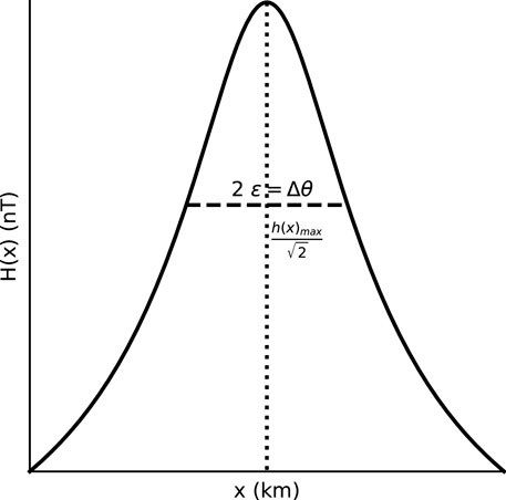
FIGURE 1. Normalised spectral amplitude profile with latitude (km) of a resonance. The characteristic latitudinal half-width, ɛ, occurs where H(x) is $\frac{1}{\sqrt{2}}$ the maximum amplitude.

The phase spectra of the north-south magnetometer component with latitude was also discussed by Baransky et al. (1989). This resonance signature can be detected by cross-phase analysis (Waters et al., 1991) of ground magnetic field data using two latitudinally separated magnetometers.

Several methods used to estimate latitudinal resonance semi-widths have been derived in the literature, based on the resonant spectral amplitude profile with latitude described by Baransky et al. (1985), Guglielmi (1989). A spectral amplitude division method (ADM) was discussed by Baransky et al. (1985, 1989) and Waters et al. (1994) and a spectral amplitude-phase method (APM) by Guglielmi (1989), Baransky et al. (1989) and Pilipenko and Fedorov (1994). The mathematical forms of the APM and ADM are given in Section 2. A hodograph method to measure the spatial resonance width was discussed by Kurchashov and Pilipenko (1996), Vellante et al. (2002) and Pilipenko et al. (2013). The hodograph method requires the complex ratio R(f) = H_P(f)/H_E(f) over a range of frequencies near a resonant frequency, f_R, where H_P and H_E are the spectral amplitudes detected at a poleward and equatorward station respectively. A circle is fit to the ratio in the complex plane, yielding a hodogram from which the resonant parameters are derived.

Another method to estimate the latitudinal resonance width was used by Walker et al. (1979), Ziesolleck et al. (1993) and Ozeke et al. (2009). This involves the full-width half-maximum (FWHM) of the spectral amplitude with latitude at a particular frequency and has been used to estimate the latitudinal resonance width of a high latitude, Pc-5 (1.5–10 mHz) FLR that occurred on the 25 November 2001 (Rae et al., 2005; Ozeke et al., 2009). Obana et al. (2015) used the APM to estimate the resonance width of low-latitude, quarter wave resonance modes that were detected using a magnetometer array in New Zealand and Takasaki et al. (2008) used this method for auroral latitude resonance events. The ADM has mostly been used to estimate latitudinal resonance widths of Pc-3 (20−100 mHz) resonances at low and mid latitudes (Waters et al., 1994; Menk et al., 2000).

Menk et al. (2000) compared results for ADM and APM estimates of resonance width for several 20 min FLR intervals across several days in April 1994 using data obtained from a low latitude array of magnetometers along eastern Australia. Uncertainty bounds of one standard deviation were included and it was found that the two methods provided similar estimates for the resonance widths. Comparisons between all three methods have not been reported. Furthermore, there are no reported studies that compare the latitudinal resonance width estimates for any of the methods at different latitudes where the Alfvén speed gradient may be different. The present methods for estimating latitudinal resonance width give a spatial estimate (km, degrees, L).

This paper compares three methods used to estimate the latitudinal width (km) of field line resonant, magnetic field signatures detected by ground magnetometers. Six intervals are discussed in detail. These used ground magnetometer data for 25 November 2001 (Rae et al., 2005; Ozeke et al., 2009), 1 October 2012 (Warden et al., 2021), and 19 June 2015. The FLR signatures from the 25 November 2001 and 1 October 2012 intervals were high latitude, Pc-5 ULF signatures detected by the CARISMA magnetometer array in Canada (Mann et al., 2008) and the Fairbanks Alaskan magnetometer array. Signatures from four different latitudes were examined for the 19 June 2015 interval, one at low latitude detected by the EMMA array (Lichtenberger et al., 2013), two at mid-latitudes detected by the IMAGE array, and a high latitude signature detected by the IMAGE array (Tanskanen, 2009). The three methods were also applied to the time series response from a driven damped harmonic oscillator model (Orr and Hanson, 1981; Gough and Orr, 1984) with known damping coefficient.

2 Methods to Estimate Latitudinal Resonance Width

In order to estimate the latitudinal resonance width, Δθ, using the FWHM the spectral amplitudes from a latitudinal array of magnetometers at the same frequency are recorded. From the spectral amplitude with magnetic latitude (MLat) curve, the locations in MLat of the −3 dB power, or $\frac{1}{\sqrt{2}}$ of maximum amplitude, are found. This yields the latitudinal resonance width, Δθ in degrees which can be converted to L shell or distance (km).

The ADM and APM resonance width estimates are derived from the FLR amplitude with frequency profile using the north-south (H) magnetometer component time series (Baransky et al., 1989; Guglielmi, 1989; Pilipenko et al., 1994). Two latitudinally separated locations, denoted poleward and equatorward, give the peak spectral amplitudes, H_P(f) and H_E(f), respectively, of the FLR profile at different frequencies, with higher frequency peaks usually located at lower latitudes and vice versa. The symbols and equations have previously used north and south subscripts [e.g., H_N(f), H_S(f) (Baransky et al., 1989)]. However, poleward (P) and equatorward (E) subscripts are used here in order to generalise the method for ground based measurements in both north and south hemispheres. The ratio, G(f) = H_P(f)/H_E(f), of these two amplitude spectra has extrema values at $x_R(f_P(f_E))=x\pm \left(\sqrt{{(\mathrm{\Delta }x/2)}^2+{\epsilon }^2}-\mathrm{\Delta }x/2\right)$ , where Δx is the station separation. These extrema have been labelled G₊ for the maximum value near f_P and G₋ for the minimum near f_E (Vellante et al., 2002). Ideally, two conditions should hold; 1) the ratio, G(f), is unity at the resonant frequency located midway between the poleward and equatorward locations, 2) G₊G₋ = 1, with a further condition that $G_{+}-G_{-}=\frac{\mathrm{\Delta }x}{\epsilon }$.

The APM uses the amplitude and phase characteristics of the resonance with frequency. The resonant frequency is identified where the cross-phase, Δϕ, is an extrema. Pilipenko and Fedorov (Pilipenko et al., 1994) derived the APM estimate for the latitudinal width in units of L shell, based on the analysis of Guglielmi (1989) and is given by

$\frac{ϵ}{\mathrm{\Delta }L}=\frac{G\sin \left(\mathrm{\Delta }\varphi \right)}{G^2-2G\cos \left(\mathrm{\Delta }\varphi \right)+1},(4)$

where ΔL is the distance between the two magnetometers (L shell separation), and G is the spectral amplitude ratio value at the resonant frequency.

The ADM for estimating the resonance width was described by Baransky et al. (1989) and used by Waters et al. (1994). This is given by

${\epsilon }^2={\left[\frac{-\beta \left(1+G_{+}^2\right)}{1-G_{+}^2}\right]}^2-{\beta }^2,(5)$

where β is half the separation between the poleward and equatorward magnetometers, in km. The ADM estimate does not use the cross-phase. The ADM and APM methods yield estimates for the half-width of the resonance, ɛ, which is half the resonance width, Δθ. All resonance width values in km, L or degrees latitude from here on are given as the full width, 2ɛ = Δθ as shown in Figure 1.

3 Results

The Pc5 interval discussed by Ozeke et al. (2009) was selected for study due to the relatively large amplitude and clear cross-phase signature at 1.5 mHz using the GIM (66.16 MLat) and ISL (63.70 MLat) magnetometers in the CARISMA magnetometer chain. The second interval was selected from the 106 FLR intervals described by Warden et al. (2021), occurring between 1800 and 1830 UT on 1 October 2012, detected by the Fairbanks Alaskan magnetometer chain, with cross-phase peak at 4.44 mHz between FYU (66.82 MLat):CMO (65.45 MLat). The third interval occurred between 0600 and 0700 UT, 19 June 2015 which showed resonant cross-phase signatures at four different latitudes. A high latitude pair, IVA (65.78 MLat) and SOD (64.41 MLat) detected a resonant frequency of 9.5 mHz and a low latitude pair, BEL (47.65 MLat) and ZAG (45.89 MLat) showed a resonant frequency of ≈25 mHz. Two middle latitude magnetometer pairs, NUR (57.06 MLat):TAR (54.66 MLat) and RAN (62.42 MLat):OUJ (61.20 MLat) showed resonances at ≈15 and 11 mHz, respectively. The magnetometers used are listed in Table 1. Time series plots for the 25 November 2001, 1 October 2012, and the four 19 June 2015 intervals are shown in Figures 2C–7C.

TABLE 1

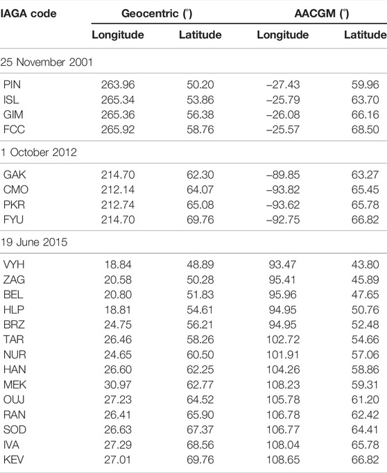
TABLE 1. Magnetometers in the CARISMA, Alaskan Fairbanks, EMMA and IMAGE magnetometer chains. The geocentric, and AACGM longitudes and latitudes are listed for each station.

FIGURE 2

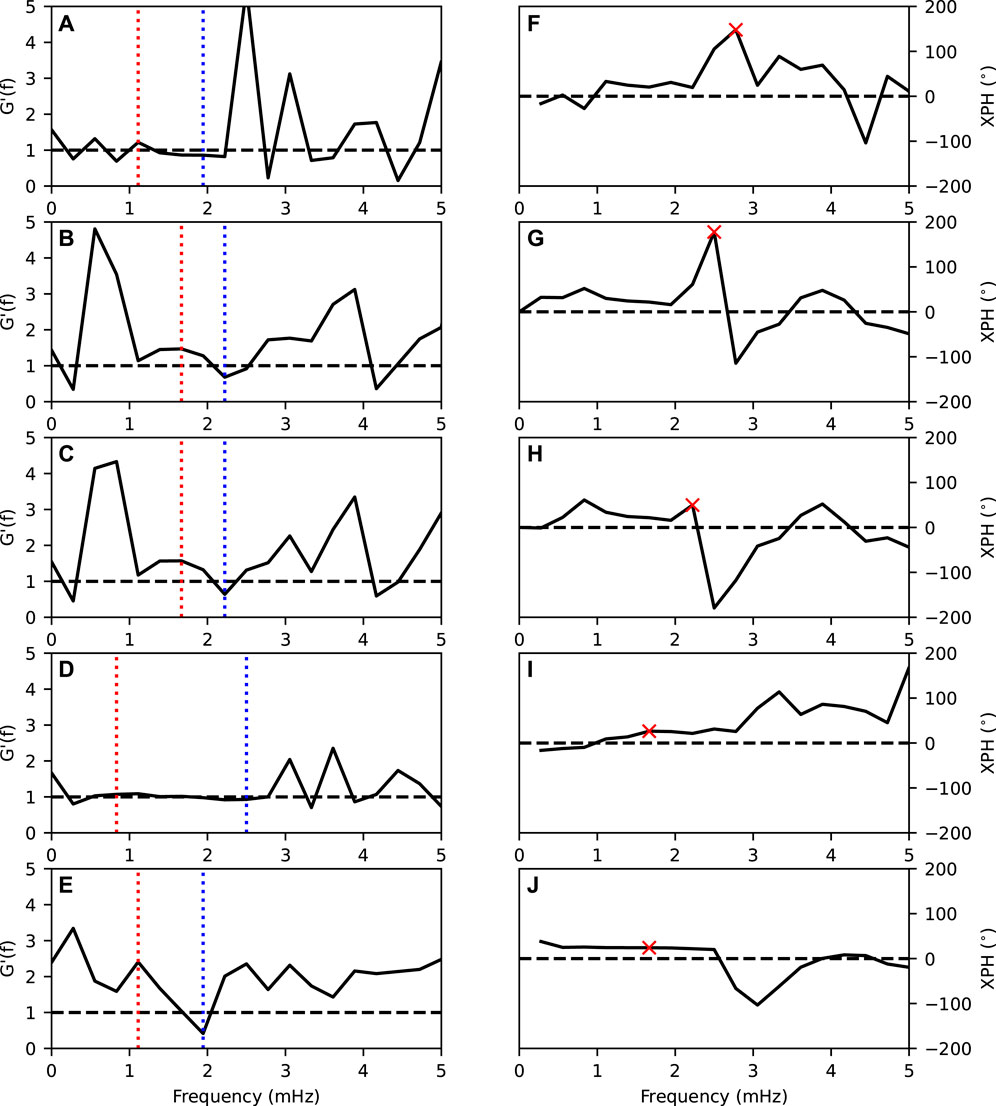
FIGURE 2. Corrected spectral amplitude ratio, G′(f), and cross-phase between GIM and ISL for the 25 November, 2001 interval for each of the five data processing methods. (A–E) correspond to G(f) for the boxcar, Hann, Hamming, exponential taper, and multi-taper methods respectively, with the red (blue) dashed line corresponding to the frequency of $G_{+(-)}^{\prime }$. (F–J) are the matching cross-phases for the spectral amplitude ratios, with the cross-phase at the resonant frequency indicated by red crosses.

FIGURE 3

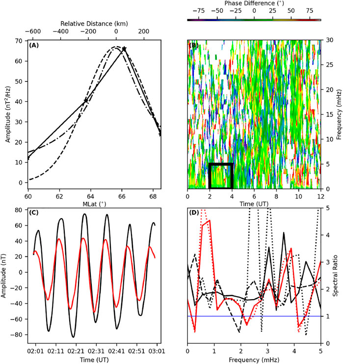
FIGURE 3. (A) Latitudinal spectral amplitude curve fits; Linear piece-wise (solid, stars at station locations), Gaussian (dashed) and FLR amplitude (Eq. 3, dash-dotted) versus MLat/km, (B) Dynamic cross phase between FYU-CMO, (C) Time series of the FYU (black) and CMO (red) magnetometer stations, and (D) Spectral amplitude ratio for the boxcar (black, dotted), Hann (red, dashed), Hamming (red, solid), exponential taper (black, solid), and multi-taper (black, dashed) FFT window processing for the FYU-CMO magnetometer data for the 1 October 2012 interval.

FIGURE 4

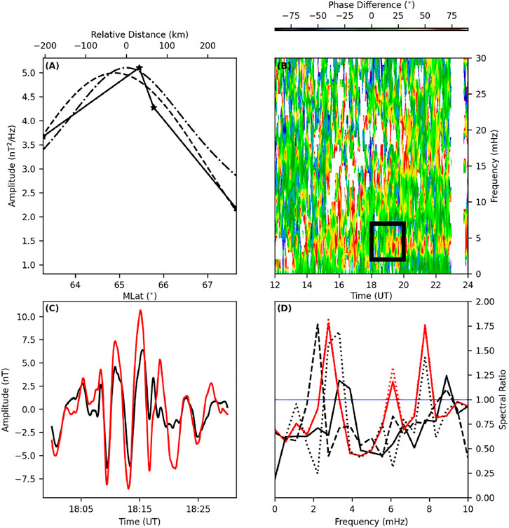
FIGURE 4. (A) Latitudinal spectral amplitude curve fits; Linear piece-wise (solid, stars at station locations), Gaussian (dashed) and FLR amplitude (Eq. 3, dash-dotted) versus MLat/km, (B) Dynamic cross phase between BEL-ZAG, (C) Time series of the BEL (black) and ZAG (red) magnetometer stations, and (D) Spectral amplitude ratio for the boxcar (black, dotted), Hann (red, dashed), Hamming (red, solid), exponential taper (black, solid), and multi-taper (black, dashed) FFT window processing for the BEL-ZAG magnetometer data for the 19 June 2015 interval.

FIGURE 5

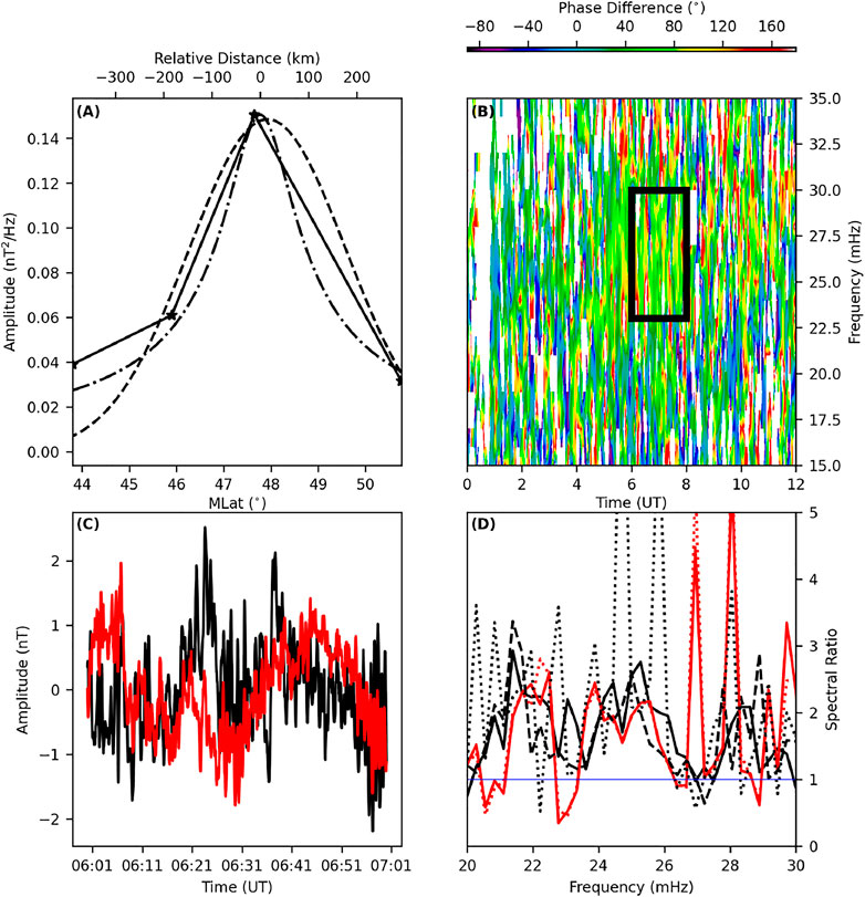
FIGURE 5. (A) Latitudinal spectral amplitude curve fits; Linear piece-wise (solid, stars at station locations), Gaussian (dashed) and FLR amplitude (Eq. 3, dash-dotted) versus MLat/km, (B) Dynamic cross phase between NUR-TAR, (C) Time series of the NUR (black) and TAR (red) magnetometer stations, and (D) Spectral amplitude ratio for the boxcar (black, dotted), Hann (red, dashed), Hamming (red, solid), exponential taper (black, solid), and multi-taper (black, dashed) FFT window processing for the NUR-TAR magnetometer data for the 19 June 2015 interval.

FIGURE 6

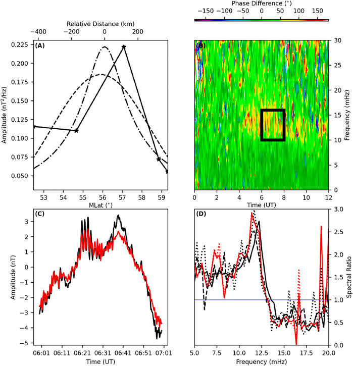
FIGURE 6. (A) Latitudinal spectral amplitude curve fits; Linear piece-wise (solid, stars at station locations), Gaussian (dashed) and FLR amplitude (Eq. 3, dash-dotted) versus MLat/km, (B) Dynamic cross phase between RAN-OUJ, (C) Time series of the RAN (black) and OUJ (red) magnetometer stations, and (D) Spectral amplitude ratio for the boxcar (black, dotted), Hann (red, dashed), Hamming (red, solid), exponential taper (black, solid), and multi-taper (black, dashed) FFT window processing for the RAN-OUJ magnetometer data for the 19 June 2015 interval.

FIGURE 7

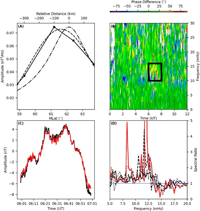
FIGURE 7. (A) Latitudinal spectral amplitude curve fits; Linear piece-wise (solid, stars at station locations), Gaussian (dashed) and FLR amplitude (Eq. 3, dash-dotted) versus MLat/km, (B) Dynamic cross phase between IVA-SOD, (C) Time series of the IVA (black) and SOD (red) magnetometer stations, and (D) Spectral amplitude ratio for the boxcar (black, dotted), Hann (red, dashed), Hamming (red, solid), exponential taper (black, solid), and multi-taper (black, dashed) FFT window processing for the IVA-SOD magnetometer data for the 19 June 2015 interval.

3.1 Amplitude With Latitude Method

The FWHM method requires three or more stations that straddle the magnetic footprint of the detected resonant frequency. For the 25 November 2001 interval Rae et al. (2005), Ozeke et al. (2009), the magnetometer stations from the CARISMA chain listed in Table 1 were used. The process used by Ozeke et al. (2009) required the maximum time series amplitudes. The maximum amplitude in the time series occurred at 0235 UT ($\approx 72$ nT) in the GIM magnetometer data (Figure 2C). The corresponding peak amplitude values in the time series from the other magnetometers around this time were selected. The FWHM was then calculated via a linear piece-wise fit to the amplitude versus the station MLat. However, Warden et al. (2021) showed that a better method was to use the spectral amplitudes at the resonance frequency in order to capture the resonance wave power rather than using a single value from the time series.

In order to calculate the spectral amplitudes, the 5 s sampled data between 0200 and 0300 UT, 25 November 2001 were multiplied by a 3,600 s boxcar window. A fast Fourier transform (FFT) of these windowed data was calculated, and the spectral amplitude at 1.5 mHz was recorded for each magnetometer. These spectral amplitudes plotted against station MLat are shown in Figure 2A. The FWHM was calculated by finding the MLat of the linear piece-wise function where the amplitude was $\frac{1}{\sqrt{2}}$ of the maximum. The MLat difference was 2.9° between these two points which was converted to km to yield a latitudinal resonance width, 2ɛ = 323 ± 138 km. The uncertainty was obtained from an analysis of the 2ɛ values at the 2σ level and is described in Section 4.

A Gaussian function was fit to the amplitude with MLat data, bounded by the most equatorward and poleward stations, PIN and FCC respectively. This was used to investigate variations in the latitudinal resonance width for different curve fit functions to the amplitude profile with latitude. The FWHM was calculated using the $\frac{1}{\sqrt{2}}$ levels from the maximum amplitude of the Gaussian fit. The uncertainty in the resonance width from the Gaussian fit was obtained from the 1.96 σ values of the Gaussian curve fit coefficients. This yielded 2ɛ = 373 ± 163 km. This was repeated using the FLR amplitude profile given by Eq. 3. Since Eq. 3 provides the amplitude profile in units of km, not MLat, the relative distance in km from the most equatorward station (PIN) to the other stations was calculated using the great-circle distance. The uncertainties were obtained using the same method as the Gaussian curve fit. The FLR amplitude fit yielded 2ɛ = 294 ± 80 km. The amplitude points and curve fits are shown in Figure 2A.

3.2 Amplitude Division and Amplitude-Phase Methods

The APM and ADM estimates require a magnetometer pair that straddles the location of a resonance. For the 25 November 2001 interval the GIM and ISL stations were selected for analysis. The time series data were processed using an FFT and five typical window functions were considered. These were boxcar, Hann, and Hamming windows (Harris, 1978), a frequency domain 3 point exponential taper smoothing algorithm (Samson and Olson, 1981), and a multi-taper average (Slepian, 1978; Thomson, 1982). These are common FFT smoothing algorithms used to reduce variance in the spectral estimates.

The GIM and ISL north-south magnetic field time series data for 0200–0300 UT, 25 November 2001 were processed by an FFT with no applied window (i.e., boxcar). There was no unit crossing near the cross-phase peak so no resonant width estimate for the ADM and APM. However, Green et al. (1993) described a method for determining a new reference level to ensure a unit crossing between G₊ and G₋. The reference level is defined as $M={(G_{+}{G}_{-})}^{1/2}$. New values of the spectral amplitude ratio, $G_{+(-)}^{\prime }$, are defined by $G_{+(-)}^{\prime }=G_{+(-)}/M$. This modification also sets the condition $G_{+}^{\prime }{G}_{-}^{\prime }=1$, and has been used for all subsequent analyses. For the boxcar FFT window, the reference level was M = 1.848 (Figure 8A), which resulted in $G_{+}^{\prime }=1.218$ and $G_{-}^{\prime }=0.821$. The cross-phase peak of 147° (Figure 8F) was observed at a resonant frequency of 2.78 mHz. From these values, 2ɛ was 54 km using the APM estimate and 1,411 km for the ADM estimate. The large discrepancy between these resonance width estimates is discussed in Section 4.

FIGURE 8

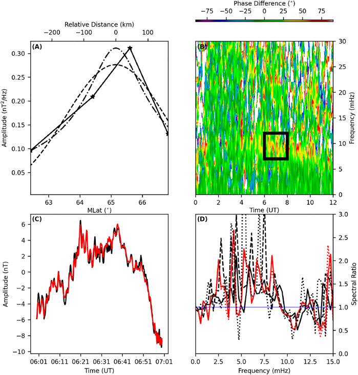
FIGURE 8. (A) Latitudinal spectral amplitude curve fits; Linear piece‐wise (solid, stars at station locations), Gaussian (dashed) and FLR amplitude (Eq. 3, dash‐dotted) versus MLat/km, (B) Dynamic cross phase between GIM‐ISL, (C) Time series of the GIM (black) and ISL (red)magnetometer stations, and (D) Spectral amplitude ratio for the boxcar (black, dotted), Hann (red, dashed), Hamming (red, solid), exponential taper (black, solid), and multi‐taper (black, dashed) FFT window processing forthe GIM‐ISL magnetometer data for the 25 November 2001 interval.

The same time series data were processed using a Hann FFT window. From this analysis, $G_{+}^{\prime }=1.47$, $G_{-}^{\prime }=0.68$ (Figure 8B) with a peak cross-phase of 178° at 2.5 mHz (Figure 8G). The Hann FFT window analysis yielded an APM estimate of 2ɛ = 6 km and an ADM estimate of 2ɛ = 711 km. The ADM estimate is approximately half the value obtained using the boxcar FFT window, while the APM estimate is an order of magnitude smaller.

Similarly to the Hann FFT window, the GIM and ISL north-south magnetic field data were multiplied by a 3,600 s Hamming window. The spectral amplitudes and cross-phase were calculated from the FFT. The resonant frequency from the spectral amplitude unity crossing and cross-phase peak was 2.2 mHz with a cross-phase peak value of 49.7° (Figure 8H). From the spectral amplitude ratios, G^′ = 1.61 and $G_{-}^{\prime }=0.63$ (Figure 8C). From these values, 2ɛ = 540 km using the APM, and 2ɛ = 574 km using the ADM estimate. This ADM estimate is approximately half the ADM boxcar FFT estimate (1,411 km), while the Hamming window, APM estimate is an order of magnitude larger than the APM boxcar FFT estimate.

Applying a window function in the time domain smooths in the frequency domain. A smoothing algorithm may be applied directly in the frequency domain. An example is the exponential taper (e.g., Samson and Olson, 1981). The boxcar windowed time series was processed by the FFT. An 3-point wide, exponential taper was used to smooth the complex spectra. This FFT window method was applied to the 25 November 2001 data. The spectral amplitude ratios were $G_{+}^{\prime }=1.09$ and $G_{-}^{\prime }=0.919$ (Figure 8C), with a unity crossing at $\approx 1.82$ mHz for the scaled $G_{+}^{\prime }$ and $G_{-}^{\prime }$. With a cross phase value of Δϕ = 24.6° (Figure 8I), the APM estimate was 198 km and ADM estimate was 3,306 km, with the ADM estimate approximately twice the boxcar ADM estimate and four times the Hann and Hamming window estimates.

The multi-taper method for improved estimates of the spectrum was described by Thomson (1982) and has been used on ULF time series (e.g., Stephenson and Walker, 2010). An algorithm for generating the window functions was described by Gruenbacher and Hummels (1994). Percival (1993) discussed a choice of parameters from a time bandwidth product, NWΔt, where N is the number of samples spaced in Δt and W is the half bandwidth. The parameters chosen for this interval were based on NWΔt = 4, with N = 720, ΔT = 5. Suitable window tapers for spectral energy within the window have eigenvalues $\approx 1$ (Percival, 1993) and the number of windows, K, where this condition holds is given by K < 2 NWΔt. For the multi-tapers applied in this study, the tapers with eigenvalues $>0.985$ were selected, resulting in four window tapers. The orthogonal time series windows were generated and the spectra of each of the windowed time series data were averaged to obtain the spectral amplitude ratio and cross-phase. From this analysis, a unity crossing in the spectral amplitude ratio occurred at ≈1.9 mHz, with a corresponding cross-phase Δϕ = 24°, as shown in Figures 8E,I, respectively. The multi-taper processing yielded APM and ADM estimates of 2ɛ = 259 km and 2ɛ = 282 km, respectively. A summary of this interval is shown in Figure 3.

The data for 1 October 2012 are shown in Figure 3. The 1 s sampled data between 1800 and 1830 UT for the north-south magnetometer components were analysed using the same processes as described above. The data for the 19 June 2015 are shown in Figures 4–7 and were analysed in a similar way. The 2ɛ results for all intervals and methods are listed in Table 2 for the FHWM and Table 3 for the APM/ADM. The FWHM width estimates for 25 November 2001 agree within uncertainty bounds. However, this is not the case for 19 June 2015 cases.

TABLE 2

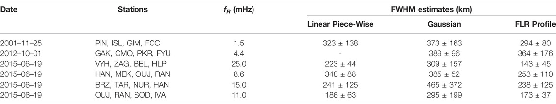
TABLE 2. Latitudinal resonance width (2ɛ, km) estimates using the FHWM method for each of the six selected intervals, with the linear piece-wise, Gaussian and Eq. 3 curve fits.

TABLE 3

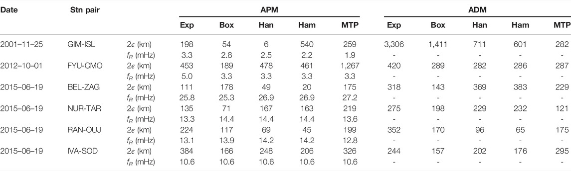
TABLE 3. APM and ADM latitudinal resonance width (2ɛ) estimates (km) for all six FLR intervals.

4 Discussion

Tables 2 and 3 show a range of values for the resonance width, for the same FLR interval. These data show that both the FFT window and choice of FWHM, APM, or ADM affects the resonance width estimates. The FWHM estimates (Table 2) show the smallest variation within a particular data interval, with the Gaussian function fits tending to yield the largest estimates for 2ɛ from the three curve fits. This may be related to the larger RMSE values for the Gaussian function fit to the spectral amplitude data compared with the fit from Eq. 3.

The APM and ADM estimates varied for the different FFT windows. The largest variation in the ADM resonance width estimates occurred where the reference level produced $G_{+}^{\prime }$ and $G_{-}^{\prime }$ close to unity. This occurred for the 25 November 2001 interval exponential taper and boxcar window, which yielded estimates from 1,411 to 3,306 km. The modified spectral ratio values were $G_{+}^{\prime }=1.09$ and $G_{-}^{\prime }=0.919$. For G₊ ≈ 1, the denominator in Eq. 5 approaches zero and the resulting resonance width estimate increases. For Eq. 4, as G′(f) decreases past unity, the width is dependent on the cross-phase and station separation, and due to the sine in the numerator, and cosine in the denominator of Eq. 4, larger cross-phase peak values yield smaller resonance width estimates. This dependence on the cross-phase at the resonant frequency gives the discrepancy between the APM and ADM estimates for the 25 November 2001 interval using a boxcar FFT window.

4.1 Driven Damped Harmonic Oscillator Model of FLRs

Given the variation in the resonance width values, without prior knowledge of the damping coefficient, it is difficult to determine which estimation method or FFT window accurately estimates the resonance width of FLR resonances. In order to progress, a computer simulation of FLRs using a magnetohydrodynamic ULF wave propagation model (Waters and Sciffer, 2008) was considered. The difficulty with this approach is the unknown FLR damping coefficient in the simulation. A simpler approach was to consider the driven damped harmonic oscillator model. Orr and Hanson (1981) and Gough and Orr (1984) described the FLR magnetic field time series response, driven at angular frequency, ω_D, modelled as

$\ddot{b_p}+2\gamma \dot{b_p}+{\omega }_0^2{b}_p={\omega }_0^2{b}_D\cos \left({\omega }_{D}t\right),(6)$

where b_p is the transverse magnetic field time series response, γ is the damping coefficient, ω₀ is the natural angular frequency of the resonant field line, b_D is the magnetic field driver amplitude, and ω_D is the angular driving frequency. The steady state solution to Eq. 6 is

$b_p=\frac{{\omega }_0^2{b}_D}{{\left({\left({\omega }_0^2-{\omega }_D^2\right)}^2+\left(4.0{\gamma }^2{\omega }_D^2\right)\right)}^{1/2}}\cos \left({\omega }_{D}t-\varphi \right),(7)$

where ϕ is given by

$\varphi ={\tan }^{-1}\left(\frac{2\gamma {\omega }_D}{{\omega }_0^2-{\omega }_D^2}\right).(8)$

The APM, ADM and FWHM provide resonance widths in distance (km or L) while Eq. 7 has the damping coefficient in s⁻¹. The relationship between the spatial and temporal damping factors depends on the resonance model and the latitudinal resonance profile as discussed, for example, by Yumoto et al. (1995). In order to determine the resonant frequencies, ω₀, for Eq. 7 and provide the mapping between the spatial resonance widths and temporal damping coefficient, a radial Alfvén velocity profile was generated using the International Reference Ionosphere (IRI) and the Field Line Interhemisphere Plasma model (FLIP; Richards et al., 2009) for the 19 June 2015 interval. A quadratic polynomial was fit to a low-latitude portion of this profile, between 2.07 and 2.92 R_E. This provided the mapping of resonant frequency to L shell as shown in Figure 9. By generating the amplitude and phase with frequency using Eq. 7 over a range of L values, according to the mapping provided by the IRI and FLIP plasma mass densities, amplitudes (and phases) with both frequency and L were obtained. The damping coefficient can be mapped from s⁻¹ into km or L by scanning in latitude, at f_R, for the $1/\sqrt{2}$ amplitudes.

FIGURE 9

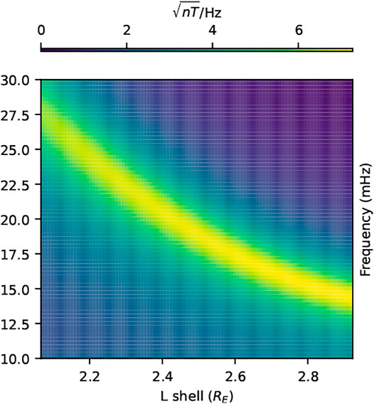
FIGURE 9. Amplitudes calculated from Eq. 7 mapped between 2.07 and 2.92 R_E using the FLR with L profile for 19 June 2015.

Equation 7 was used to investigate the effects of data processing and resonance width method (FWHM, ADM, APM) on estimates of Δθ, given the known damping. For the ADM and APM, two L shell locations were selected as ground station locations, a poleward point at 2.55 R_E and an equatorward point at 2.44 R_E with resonant frequencies of 18.3 and 20.0 mHz, respectively. These locations provided estimates of the input damping at a resonant frequency, f_R = 19.1 mHz, mid-way between the locations. The time series responses to a broad-band driver spectrum between 10 and 30 mHz were generated using Eq. 7, with b_D = 1. The phase spectra from the poleward and equatorward locations were unwrapped then subtracted to provide the phase difference with frequency. The phase difference at f_R was used as Δϕ in Eq. 4. The FWHM method was simulated by generating the time series response for every point in the resonant frequency latitudinal profile, and calculating the FWHM for the spectral amplitudes recorded at the 19.1 mHz frequency. Two cases were considered for the damping coefficient; $\frac{\gamma }{{\omega }_0}=0.1$ as typical reported day-time values (Orr and Hanson, 1981; Gough and Orr, 1984) and $\frac{\gamma }{{\omega }_0}=0.055$ (Walker et al., 1979). Table 4 lists the latitudinal resonance widths (km) obtained from Eq. 7 time series resonance response using the same processes described in Section 3.

TABLE 4

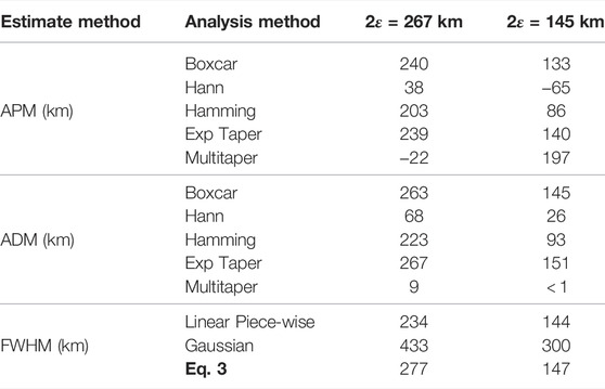
TABLE 4. APM, ADM, and FWHM estimates of the latitudinal resonance width in km, with uncertainty, for the driven damped harmonic oscillator model. 2ɛ = 267 km corresponds to the γ/ω₀ = 0.1 case, and 2ɛ = 145 km corresponds to the γ/ω₀ = 0.055 case.

From the results in Table 4, the boxcar and exponential taper FFT window functions gave the most accurate estimates for ADM methods, close to the actual value for the smaller spatial damping coefficient of 2ɛ = 145 km. The Hamming FFT window function gave the next best estimates. The Hann window and multi-taper algorithms gave the least accurate results, underestimating the resonance width. While the APM estimates followed a similar trend in which processing methods yielded the most accurate results, these estimates tended to underestimate 2ɛ to a greater extent compared with the ADM. The Hann FFT window and APM underestimated the resonance width for the 2ɛ = 267 km case, and gave a non-physical, negative resonance width for the 2ɛ = 145 km case. The multi-taper and APM width estimate was negative for the 2ɛ = 267 km damping case and over-estimated for the 2ɛ = 145 km damping case. These Hann window and multi-taper based estimates are discussed further in Section 4.2. Comparison of the window function methods between the APM and ADM show that the boxcar, exponential taper, and Hamming window smoothing methods give similar results between the two estimation methods.

For the FWHM, Eq. 3, and linear piece-wise curve fits yielded the most accurate estimates of 2ɛ. The Gaussian curve fit gave up to twice the expected values for both 2ɛ cases. The linear piece-wise curve fit depends on the spatial resolution of the magnetometer station chain. Therefore, the accuracy of the estimates obtained from the linear piece-wise fit in this driven damped harmonic oscillator model may not be realised in practice given the relatively sparse spatial measurements.

Comparison of the data analysis techniques for all three resonance width estimate methods shows that the ADM and FWHM tend to over-estimate 2ɛ calculated from the real γ, while the APM underestimates this value. However, the uncertainties for the APM and ADM using the boxcar FFT window function and exponential smoothing taper, and the FWHM linear piece-wise and Eq. 3 curve fits estimates covered the real γ value.

4.2 FFT Window Effects

For the APM and ADM estimates, details of the spectra reveal why the Hann, Hamming and multi-taper window functions yielded quite different results. These methods use information from closely spaced magnetometers which translates to a narrow band in the spectrum. Figure 10 shows the amplitude spectra at the poleward and equatorward points, and the corresponding cross-phase for the 2ɛ = 145 km and 2ɛ = 267 km damping cases from the driven damped harmonic oscillator model. For the multi-taper, Hann and Hamming windows, the amplitude spectra have a sharper decrease in amplitude away from the resonant frequency at 19.1 mHz, relative to the exponential taper and boxcar window functions. The convolution in the frequency domain of the FFT window and the data mixes adjacent frequency components into the spectra, which are then divided to obtain G₊ and G₋. This combined process for the Hann and multi-taper windows gives larger differences between the estimated and known values for the resonance width for the driven damped harmonic oscillator model.

FIGURE 10

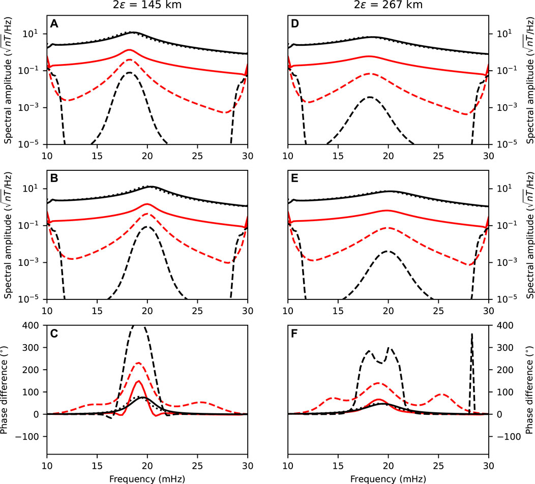
FIGURE 10. Amplitude and phase spectra from the driven damped harmonic oscillator model with different window tapers applied to data. Panels (A,B) show the amplitude spectra for the poleward and equatorward stations, respectively, for damping coefficient, 2ɛ = 145 km. Panel (C) the cross-phase between the phase spectra in panels (A,B). Panels (D–F) follow the same layout for a damping coefficient value of 2ɛ = 267 km. The lines correspond to the following - boxcar (black, dotted), Hann (red, dashed), Hamming (red, solid), exponential taper (black, solid), and multi-taper (black, dashed) processing methods.

The convolution in the frequency domain also affects the cross-phase. From the damped harmonic oscillator model, the cross-phase values were 70 and 50° for 2ɛ equal to 145 and 267 km, respectively. Figures 10C,F shows that the cross-phase values at f_R for the Hann and multi-taper windows were larger than the known values. The cross-phase value at f_R from the Hamming window for the 2ɛ = 145 km was larger compared to the known value. These larger values of the cross-phase give smaller estimates for the resonance width from the APM. For phase differences between 180 and 360° obtained from the unwrapped phase, the resonance width is negative from the APM. The phase of the harmonic oscillator depends on the driving frequency, natural frequency of the resonant system and the damping coefficient. From Eq. 8, when ω_D = ω₀, $\frac{d\varphi }{d{\omega }_D}=\frac{1}{\gamma }$. This inverse dependence on the damping coefficient shows that the phase change over the resonant frequency occurs over a narrower bandwidth for decreased damping. The phase mixing from the convolution of the FFT of the signal and window has a greater impact on the phase difference for smaller damping coefficients.

4.3 Uncertainty Analysis

Independent of the FFT window processing, the uncertainty of the ADM estimate for ɛ depends on the spectral amplitudes and the ratio, G₊. Figure 11A shows an example of how the ADM estimate for the resonance width changes with G₊, using a typical station spacing, β, of 200 km. For G₊ values near unity, there are large changes in ɛ for small changes in G₊. For G₊ larger than unity, the rate of change of ɛ is smaller for similar uncertainties in G₊. This means that the uncertainties in ɛ depend on how close G₊ is to unity. This section is a description of an uncertainty analysis to determine this dependence.

FIGURE 11

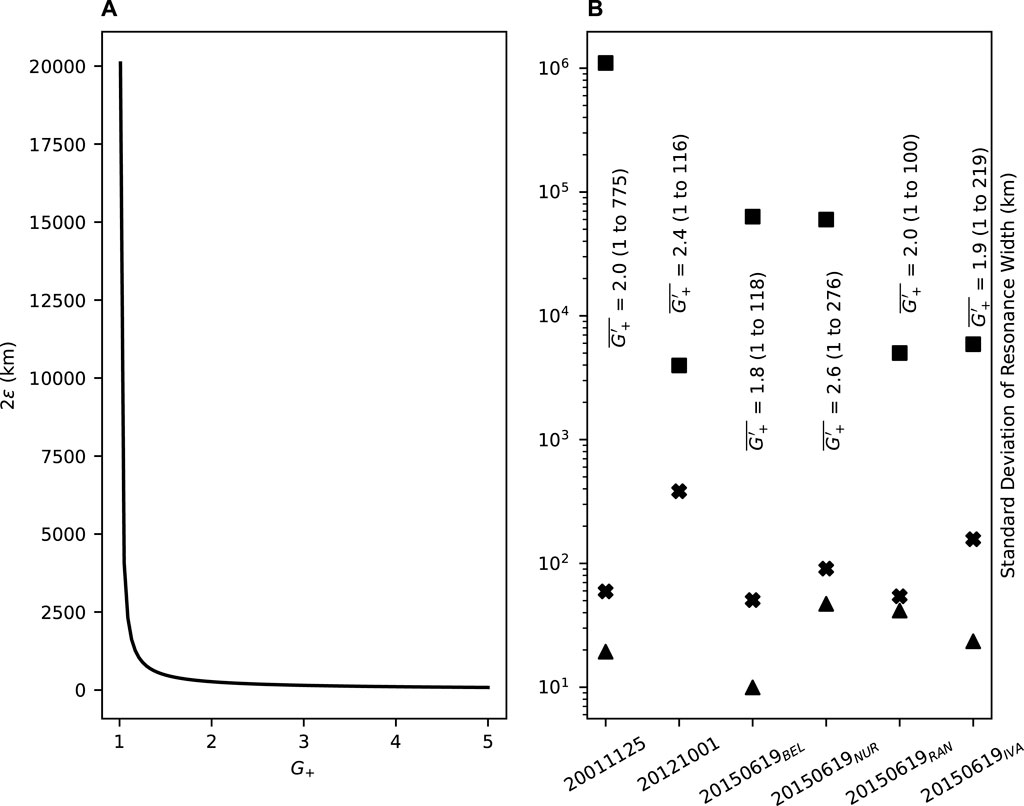
FIGURE 11. (A) Plot of the variation of 2ɛ with G₊ from Eq. 5, with β = 200 km. (B) Standard deviations of the 2ɛ distributions for the FWHM (triangle), APM (cross), and ADM (square) obtained from σ_amp = 15% for the 25 November 2001, 1 October 2012, and the four latitudinal slices of the 19 June 2015 interval. The means $(\overline{G_{+}^{\prime }})$ and ranges of $G_{+}^{\prime }$ are also shown.

For the FWHM method, the boxcar FFT window spectral amplitudes at 1.39 mHz were used from the 25 November 2001 interval. The spectral amplitudes were sampled 10⁵ times from a normal distribution. The means were set to the experimental values for each station and the standard deviation was set to different percentages of the amplitude recorded at PIN. The case for the standard deviation set to 15% is shown in Figure 11B. The FWHM was calculated using the linear piece-wise curve fit, and the standard deviation of the resonance width estimates was calculated.

This process was repeated for the APM and ADM resonance width estimates, using the experimental spectral amplitudes from the GIL-ISL station pair at the frequencies, f₊ and f₋. The standard deviation of the normal distribution was set to 15% of the recorded spectral amplitude at the f₊ frequency at the poleward station, GIL. The APM also required the cross-phase distribution. The cross-phase recorded at 1.5 mHz was set as the mean cross-phase with 15% of this cross-phase used for the standard deviation. The uncertainty analysis was repeated for the remaining intervals following the same process. Figure 11B shows the results of this uncertainty analysis for all three estimate methods for all intervals.

As seen in Figure 11B, the FWHM and APM estimates of the resonance width result in the smallest standard deviations. The ADM has the largest standard deviation range in the resonance width estimate, due to the large proportion of $G_{+}^{\prime }$ near unity. In the damped driven harmonic oscillator model, the ADM, using a boxcar FFT window or exponential taper, gave the closest estimates to the known resonance width due to $G_{+}^{\prime }$ being sufficiently far from unity. For the boxcar FFT window, these were 2.6 and 1.6 for the 2ɛ equal to 145 and 267 km, respectively. The results of the uncertainty analysis reinforce the condition that G₊ should be sufficiently larger than unity for the ADM. How much larger than unity depends on the resonance width.

A major limitation on the FWHM method is the availability of a closely spaced, latitudinally separated chain of magnetometers. This method requires a chain of magnetometers, preferably within 500 km of an FLR footprint, that adequately sample the latitudinal profile of the resonance. The more stations that can be used the better the resolution of the FLR profile with latitude. This requirement is less problematic for FLRs detected in the northern hemisphere over North America, Europe and Asia, but limits the application of this method for studies using southern hemisphere chains where the magnetometer networks are sparse.

Hodograms were also generated for each of the intervals, following the process outlined by Pilipenko et al. (2013). A requirement of the hodograph method is that the complex ratio, H_P/H_E should vary smoothly around a circle in the complex plane over the range of frequencies in the vicinity of the resonance. However, this was not the case for the selected data intervals. Furthermore, the number of complex points is small for resonance signatures in the Pc5 range which limits the number of points to fit. Deviations from the circular resonance profile for the hodograph method were observed for a resonance model that included enhanced driving frequency amplitudes over a narrow band of the excitation profile, a topic for future study.

The driven damped harmonic oscillator model and uncertainty analysis results can be used to guide the choice of estimate method and analysis technique. Where a station pair straddles a resonance and the $G_{+}^{\prime }$ ratio is sufficiently far from unity, the ADM or APM, with both boxcar and exponential taper smoothing could be used to obtain estimates of the latitudinal resonance width. If a sufficiently spatially resolved chain of magnetometers is available, the FHWM estimate using an Eq. 3 curve-fit could also be used.

5 Conclusion

Three methods used to obtain the latitudinal resonance width of field line resonances from ground magnetometer data have been compared. These were a full-width half-maximum method (FWHM), amplitude-phase (APM) and amplitude-division (ADM) methods. Six FLR intervals were studied, selected from 25 November 2001, 1 October 2012, and 19 June 2015. The 19 June 2015 interval was separated into low latitude, two mid-latitude and one high latitude section. It was found that the resonance width estimates varied with the method used and the FFT data processing.

A driven damped harmonic oscillator model with known frequency and damping was used to compare the width estimation and data processing methods. From this model, it was found that the best resonance width estimates were given by the ADM when the data were processed using a boxcar smoothing window or a 3-point, frequency domain, exponential smoothing taper. However, this accuracy depends on how close $G_{+}^{\prime }$ is to unity. The APM and FWHM tended to underestimate the latitudinal resonance width. The FWHM yielded accurate results for a curve fit using Eq. 3 and a high spatial resolution linear piece-wise curve fit to the FLR profile. The other data processing techniques were found to underestimate resonance width values.

The resonance width estimates of the FLR intervals have been obtained using single sensor components of the ground magnetic field data, specifically the north-south component. The APM and ADM assume that the resonance is the dominant signal in the north-south magnetometer component between f₊ and f₋. The FWHM assumes that a resonance of f_R at some latitude L_R is the dominant signal over a range of latitudes. However, the magnetosphere supports a resonance continuum plus possible amplitude enhancements from compressional mode signals which then pass through the ionosphere which may alter estimates of the resonance width obtained at the ground. These aspects of the shear mode resonance response in the magnetosphere are for future work.

Data Availability Statement

The original contributions presented in the study are included in the article/Supplementary Material, further inquiries can be directed to the corresponding author.

Author Contributions

LW, CW, and MD conceived of and designed the scope of the study. LW wrote codes for reading/analysis of magnetometer data and the codes for model and analysis codes of the model. LW wrote the first draft of the manuscript, and LW, CW, MD, and MV contributed to editing/revisions of the manuscript and approval of the submitted version of the manuscript. MV with provision of the EMMA data.

Conflict of Interest

The authors declare that the research was conducted in the absence of any commercial or financial relationships that could be construed as a potential conflict of interest.

Publisher’s Note

All claims expressed in this article are solely those of the authors and do not necessarily represent those of their affiliated organizations, or those of the publisher, the editors and the reviewers. Any product that may be evaluated in this article, or claim that may be made by its manufacturer, is not guaranteed or endorsed by the publisher.

Acknowledgments

This research was funded under the Research Training Program Scholarship, Department of Education, Skills and Employment, Australia. CARISMA is operated by the University of Alberta, funded by the Canadian Space Agency. The IMAGE Magnetometer Array is maintained by: Tromso Geophysical Observatory of UiT, the Arctic University of Norway (Norway), Finnish Meteorological Institute (Finland), Institute of Geophysics Polish Academy of Sciences (Poland), GFZ German Research Centre for Geosciences (Germany), Geological Survey of Sweden (Sweden), Swedish Institute of Space Physics (Sweden), Sodanklya Geophysical Observatory of the University of Oulu (Finland), and Polar Geophysical Institute (Russia). EMMA Magnetometer Array is maintained by: Institute of Geophysics of the Polish Academy of Sciences (IGF-PAS), Mining and Geological Survey of Hungary (MBFSZ), University of L’Aquila, Italy. Alaskan data provided by the Geophysical Institute Magnetometer Array operated by the Geophysical Institute, University of Alaska. The authors thank the CARISMA team (http://www.carisma.ca), the IMAGE team (https://space.fmi.fi/image/), EMMA team (http://geofizika.canet.hu/plasmon/), and Geophysical Institute of UoA (https://www.gi.alaska.edu/monitors/magnetometer).

References

Baddeley, L. J., Yeoman, T. K., Wright, D. M., Trattner, K. J., and Kellet, B. J. (2004). A Statistical Study of Unstable Particle Populations in the Global Ring Current and Their Relation to the Generation of High M ULF Waves. Ann. Geophys. 22, 4229–4241. doi:10.5194/angeo-22-4229-2004

CrossRef Full Text | Google Scholar

Baransky, L. N., Belokris, S. P., Borovkov, Y. E., Gokhberg, M. B., Fedorov, E. N., and Green, C. A. (1989). Restoration of the Meridional Structure of Geomagnetic Pulsation Fields from Gradient Measurements. Planet. Space Sci. 37, 859–864. doi:10.1016/0032-0633(89)90136-0

CrossRef Full Text | Google Scholar

Baransky, L. N., Borovkov, J. E., Gokhberg, M. B., Krylov, S. M., and Troitskaya, V. A. (1985). High Resolution Method of Direct Measurement of the Magnetic Field Lines' Eigen Frequencies. Planet. Space Sci. 33, 1369–1374. doi:10.1016/0032-0633(85)90112-6

CrossRef Full Text | Google Scholar

Dai, L., Takahashi, K., Wygant, J. R., Chen, L., Bonnell, J., Cattell, C. A., et al. (2013). Excitation of Poloidal Standing Alfvén Waves through Drift Resonance Wave-Particle Interaction. Geophys. Res. Lett. 40, 4127–4132. doi:10.1002/grl.50800

CrossRef Full Text | Google Scholar

Drozdov, A. Y., Shprits, Y. Y., Aseev, N. A., Kellerman, A. C., and Reeves, G. D. (2017). Dependence of Radiation Belt Simulations to Assumed Radial Diffusion Rates Tested for Two Empirical Models of Radial Transport. Space Weather 15, 150–162. doi:10.1002/2016sw001426

CrossRef Full Text | Google Scholar

Gough, H., and Orr, D. (1984). The Effect of Damping on Geomagnetic Pulsation Amplitude and Phase at Ground Observatories. Planet. Space Sci. 32, 619–628. doi:10.1016/0032-0633(84)90112-0

CrossRef Full Text | Google Scholar

Green, A. W., Worthington, E. W., Baransky, L. N., Fedorov, E. N., Kurneva, N. A., Pilipenko, V. A., et al. (1993). Alfven Field Line Resonances at Low Latitudes (L= 1.5). J. Geophys. Res. 98, 15693. doi:10.1029/93ja00644

CrossRef Full Text | Google Scholar

Gruenbacher, D. M., and Hummels, D. R. (1994). A Simple Algorithm for Generating Discrete Prolate Spheroidal Sequences. IEEE Trans. Signal Process. 42, 3276–3278. doi:10.1109/78.330397

CrossRef Full Text | Google Scholar

Guglielmi, A. V. (1989). Diagnostics of the Plasma in the Magnetosphere by Means of Measurement of the Spectrum of Alfvén Oscillations. Planet. Space Sci. 37, 1011–1012. doi:10.1016/0032-0633(89)90055-x

CrossRef Full Text | Google Scholar

Harris, F. J. (1978). On the Use of Windows for Harmonic Analysis with the Discrete Fourier Transform. Proc. IEEE 66, 51–83. doi:10.1109/proc.1978.10837

CrossRef Full Text | Google Scholar

Jacobs, J. A., Kato, Y., Matsushita, S., and Troitskaya, V. A. (1964). Classification of Geomagnetic Micropulsations. J. Geophys. Res. 69, 180–181. doi:10.1029/jz069i001p00180

CrossRef Full Text | Google Scholar

Kurchashov, Y. P., and Pilipenko, V. A. (1996). Geometrical Method for the Analysis of the ULF Gradient Observation Data. Geomagn. Areon. 36, 53–60.

Google Scholar

Lichtenberger, J., Clilverd, M. A., Heilig, B., Vellante, M., Manninen, J., Rodger, C. J., et al. (2013). The Plasmasphere during a Space Weather Event: First Results from the PLASMON Project. J. Space Weather Space Clim. 3, A23. doi:10.1051/swsc/2013045

CrossRef Full Text | Google Scholar

Lifshitz, A. E., and Federov, E. N. (1986). Hydromagnetic Oscillations of the Magnetosphere-Ionosphere Resonator. Dokl. Akad. Nauk. SSSR 287, 90–94.

Google Scholar

Liu, W., Cao, J. B., Li, X., Sarris, T. E., Zong, Q.-G., Hartinger, M., et al. (2013). Poloidal ULF Wave Observed in the Plasmasphere Boundary Layer. J. Geophys. Res. Space Phys. 118, 4298–4307. doi:10.1002/jgra.50427

CrossRef Full Text | Google Scholar

Mann, I. R., Milling, D. K., Rae, I. J., Ozeke, L. G., Kale, A., Kale, Z. C., et al. (2008). The Upgraded CARISMA Magnetometer Array in the THEMIS Era. Space Sci. Rev. 141, 413–451. doi:10.1007/s11214-008-9457-6

CrossRef Full Text | Google Scholar

Mathie, R. A., and Mann, I. R. (2000). A Correlation between Extended Intervals of ULF Wave Power and Storm-Time Geosynchronous Relativistic Electron Flux Enhancements. Geophys. Res. Lett. 27, 3261–3264. doi:10.1029/2000gl003822

CrossRef Full Text | Google Scholar

Menk, F. W., Waters, C. L., and Fraser, B. J. (2000). Field Line Resonances and Waveguide Modes at Low Latitudes: 1. Observations. J. Geophys. Res. 105, 7747–7761. doi:10.1029/1999ja900268

CrossRef Full Text | Google Scholar

Murphy, K. R., Mann, I. R., and Ozeke, L. G. (2014). A ULF Wave Driver of Ring Current Energization. Geophys. Res. Lett. 41, 6595–6602. doi:10.1002/2014gl061253

CrossRef Full Text | Google Scholar

O'Brien, T. P., McPherron, R. L., Sornette, D., Reeves, G. D., Friedel, R., and Singer, H. J. (2001). Which Magnetic Storms Produce Relativistic Electrons at Geosynchronous Orbit? J. Geophys. Res. 106, 15533–15544. doi:10.1029/2001ja000052

CrossRef Full Text | Google Scholar

Obana, Y., Waters, C. L., Sciffer, M. D., Menk, F. W., Lysak, R. L., Shiokawa, K., et al. (2015). Resonance Structure and Mode Transition of Quarter‐Wave ULF Pulsations Around the Dawn Terminator. J. Geophys. Res. Space Phys. 120, 4194–4212. doi:10.1002/2015ja021096

CrossRef Full Text | Google Scholar

Olson, J. V., and Rostoker, G. (1978). Longitudinal Phase Variations of Pc 4-5 Micropulsations. J. Geophys. Res. 83, 2481. doi:10.1029/ja083ia06p02481

CrossRef Full Text | Google Scholar

Orr, D., and Hanson, H. W. (1981). Geomagnetic Pulsation Phase Patterns over an Extended Latitudinal Array. J. Atmos. Terr. Phys. 43, 899–910. doi:10.1016/0021-9169(81)90081-7

CrossRef Full Text | Google Scholar

Ozeke, L. G., Mann, I. R., Murphy, K. R., Rae, I. J., Milling, D. K., Elkington, S. R., et al. (2012). ULF Wave Derived Radiation Belt Radial Diffusion Coefficients. J. Geophys. Res. Space Phys. 117, A04222. doi:10.1029/2011ja017463

CrossRef Full Text | Google Scholar

Ozeke, L. G., Mann, I. R., Olifer, L., Dufresne, K. Y., Morley, S. K., Claudepierre, S. G., et al. (2020). Rapid Outer Radiation Belt Flux Dropouts and Fast Acceleration during the March 2015 and 2013 Storms: The Role of Ultra-low Frequency Wave Transport from a Dynamic Outer Boundary. J. Geophys. Res. Space Phys. 125, e2019JA027179. doi:10.1029/2019ja027179

CrossRef Full Text | Google Scholar

Ozeke, L. G., Mann, I. R., and Rae, I. J. (2009). Mapping Guided Alfvén Wave Magnetic Field Amplitudes Observed on the Ground to Equatorial Electric Field Amplitudes in Space. J. Geophys. Res. Space Phys. 114, A01214. doi:10.1029/2008ja013041

CrossRef Full Text | Google Scholar

Percival, D. (1993). Spectral Analysis for Physical Applications : Multitaper and Conventional Univariate Techniques. Cambridge New York, NY, USA: Cambridge University Press.

Google Scholar

Pilipenko, V. A., and Fedorov, E. N. (1994). “Magnetotelluric Sounding of the Crust and Hydrodynamic Monitoring of the Magnetosphere with the Use of ULF Waves,” in Solar Wind Sources of Magnetospheric Ultra-Low-Frequency Waves. Editors MJ Engebreston, K Takahashi, and M Scholer (Washington, DC: American Geophysical Union), 283–292. doi:10.1029/gm081p0283

CrossRef Full Text | Google Scholar

Pilipenko, V. A., Kawano, H., and Mann, I. R. (2013). Hodograph Method to Estimate the Latitudinal Profile of the Field-Line Resonance Frequency Using the Data from Two Ground Magnetometers. Earth Planet Sp. 65, 435–446. doi:10.5047/eps.2013.02.007

CrossRef Full Text | Google Scholar

Pu, Z.-Y., and Kivelson, M. G. (1983). Kelvin-Helmholtz Instability at the Magnetopause: Solution for Compressible Plasmas. J. Geophys. Res. 88, 841. doi:10.1029/ja088ia02p00841

CrossRef Full Text | Google Scholar

Rae, I. J., Donovan, E. F., Mann, I. R., Fenrich, F. R., Watt, C. E. J., Milling, D. K., et al. (2005). Evolution and Characteristics of Global Pc5 ULF Waves during a High Solar Wind Speed Interval. J. Geophys. Res. 110, A12211. doi:10.1029/2005ja011007

CrossRef Full Text | Google Scholar

Richards, P. G., Nicolls, M. J., Heinselman, C. J., Sojka, J. J., Holt, J. M., and Meier, R. R. (2009). Measured and Modeled Ionospheric Densities, Temperatures, and Winds during the International Polar Year. J. Geophys. Res. Space Phys. 114, A12317. doi:10.1029/2009ja014625

CrossRef Full Text | Google Scholar

Rostoker, G., Skone, S., and Baker, D. N. (1998). On the Origin of Relativistic Electrons in the Magnetosphere Associated with Some Geomagnetic Storms. Geophys. Res. Lett. 25, 3701–3704. doi:10.1029/98gl02801

CrossRef Full Text | Google Scholar

Samson, J. C., and Olson, J. V. (1981). Data‐adaptive Polarization Filters for Multichannel Geophysical Data. Geophysics 46, 1423–1431. doi:10.1190/1.1441149

CrossRef Full Text | Google Scholar

Samson, J. C., Waters, C. L., Menk, F. W., and Fraser, B. J. (1995). Fine Structure in the Spectra of Low Latitude Field Line Resonances. Geophys. Res. Lett. 22, 2111–2114. doi:10.1029/95gl01770

CrossRef Full Text | Google Scholar

Slepian, D. (1978). Prolate Spheroidal Wave Functions, Fourier Analysis, and Uncertainty-V: The Discrete Case. Bell Syst. Tech. J. 57, 1371–1430. doi:10.1002/j.1538-7305.1978.tb02104.x

CrossRef Full Text | Google Scholar

Southwood, D. J., and Hughes, W. J. (1983). Theory of Hydromagnetic Waves in the Magnetosphere. Space Sci. Rev. 35, 301–366. doi:10.1007/bf00169231

CrossRef Full Text | Google Scholar

Southwood, D. J. (1968). The Hydromagnetic Stability of the Magnetospheric Boundary. Planet. Space Sci. 16, 587–605. doi:10.1016/0032-0633(68)90100-1

CrossRef Full Text | Google Scholar

Stephenson, J. A. E., and Walker, A. D. M. (2010). Coherence between Radar Observations of Magnetospheric Field Line Resonances and Discrete Oscillations in the Solar Wind. Ann. Geophys. 28, 47–59. doi:10.5194/angeo-28-47-2010

CrossRef Full Text | Google Scholar

Takasaki, S., Sato, N., Kadokura, A., Yamagishi, H., Kawano, H., Ebihara, Y., et al. (2008). Interhemispheric Observations of Field Line Resonance Frequencies as a Continuous Function of Ground Latitude in the Auroral Zones. Polar Sci. 2, 73–86. doi:10.1016/j.polar.2008.05.003

CrossRef Full Text | Google Scholar

Tanskanen, E. I. (2009). A Comprehensive High-Throughput Analysis of Substorms Observed by IMAGE Magnetometer Network: Years 1993-2003 Examined. J. Geophys. Res. 114, A05204. doi:10.1029/2008ja013682

CrossRef Full Text | Google Scholar

Thomson, D. J. (1982). Spectrum Estimation and Harmonic Analysis. Proc. IEEE 70, 1055–1096. doi:10.1109/proc.1982.12433

CrossRef Full Text | Google Scholar

Vellante, M., De Lauretis, M., Förster, M., Lepidi, S., Zieger, B., Villante, U., et al. (2002). Geomagnetic Field Line Resonances at Low Latitudes: Pulsation Event Study of 16 August 1993. J. Geophys. Res. 107, SMP 6-1–SMP 6-18. doi:10.1029/2001ja900123

CrossRef Full Text | Google Scholar

Walker, A. D. M., Greenwald, R. A., Stuart, W. F., and Green, C. A. (1979). Stare Auroral Radar Observations of Pc 5 Geomagnetic Pulsations. J. Geophys. Res. 84, 3373. doi:10.1029/ja084ia07p03373

CrossRef Full Text | Google Scholar

Walker, A. D. M. (1981). The Kelvin-Helmholtz Instability in the Low-Latitude Boundary Layer. Planet. Space Sci. 29, 1119–1133. doi:10.1016/0032-0633(81)90011-8

CrossRef Full Text | Google Scholar

Warden, L. J., Waters, C. L., Sciffer, M. D., and Hull, A. J. (2021). On the Estimation of the Ratio of ULF Wave Electric Fields in Space and the Magnetic Fields at the Ground. J. Geophys. Res. Space Phys. 126, e2020JA029052. doi:10.1029/2020ja029052

CrossRef Full Text | Google Scholar

Waters, C. L., Harrold, B. G., Menk, F. W., Samson, J. C., and Fraser, B. J. (2000). Field Line Resonances and Waveguide Modes at Low Latitudes: 2. A Model. J. Geophys. Res. 105, 7763–7774. doi:10.1029/1999ja900267

CrossRef Full Text | Google Scholar

Waters, C. L., Menk, F. W., and Fraser, B. J. (1994). Low Latitude Geomagnetic Field Line Resonance: Experiment and Modeling. J. Geophys. Res. 99, 17547. doi:10.1029/94JA00252

CrossRef Full Text | Google Scholar

Waters, C. L., Menk, F. W., and Fraser, B. J. (1991). The Resonance Structure of Low Latitude Pc3 Geomagnetic Pulsations. Geophys. Res. Lett. 18, 2293–2296. doi:10.1029/91gl02550

CrossRef Full Text | Google Scholar

Waters, C. L., and Sciffer, M. D. (2008). Field Line Resonant Frequencies and Ionospheric Conductance: Results from a 2-D MHD Model. J. Geophys. Res. 113, A05219. doi:10.1029/2007ja012822

CrossRef Full Text | Google Scholar

Yumoto, K., Pilipenko, V., Federov, E., Kurneva, N., and Shiokawa, K. (1995). The Mechanisms of Damping of Geomagnetic Pulsations. J. Geomagn. Geoelectr. 47, 163–176. doi:10.5636/jgg.47.163

CrossRef Full Text | Google Scholar

Zhu, X., and Kivelson, M. G. (1988). Analytic Formulation and Quantitative Solutions of the Coupled ULF Wave Problem. J. Geophys. Res. 93, 8602. doi:10.1029/ja093ia08p08602

CrossRef Full Text | Google Scholar

Ziesolleck, C. W. S., Fraser, B. J., Menk, F. W., and McNabb, P. W. (1993). Spatial Characteristics of Low-Latitude Pc3-4 Geomagnetic Pulsations. J. Geophys. Res. 98, 197–207. doi:10.1029/92ja01433

CrossRef Full Text | Google Scholar