 Robert J. Leamon
 Scott W. McIntosh
 Alan M. Title4
95% of researchers rate our articles as excellent or good
Learn more about the work of our research integrity team to safeguard the quality of each article we publish.
Find out more
ORIGINAL RESEARCH article
Front. Astron. Space Sci. , 10 May 2022
Sec. Stellar and Solar Physics
Volume 9 - 2022 | https://doi.org/10.3389/fspas.2022.886670
This article is part of the Research Topic Short- and Long-Term Solar Activity and its Potential Influences on Earth’s Atmosphere View all 4 articles
The Sun’s variability is controlled by the progression and interaction of the magnetized systems that form the 22-year magnetic activity cycle (the “Hale Cycle”) as they march from their origin at ∼55° latitude to the equator, over ∼19 years. We will discuss the end point of that progression, dubbed “terminator” events, and our means of diagnosing them. In this paper we expand on the Extended Solar Cycle framework to construct a new solar activity “clock” which maps all solar magnetic activity onto a single normalized epoch based on the terminations of Hale Magnetic Cycles. Defining phase 0*2π on this clock as the Terminators, then solar polar field reversals occur at ∼ 0.2*2π, and the geomagnetically quiet intervals centered around solar minimum start at ∼ 0.6*2π and end at the terminator, thus lasting 40% of the cycle length. At this onset of quiescence, dubbed a “pre-terminator,” the Sun shows a radical reduction in active region complexity and, like the terminator events, is associated with the time when the solar radio flux crosses F10.7 = 90 sfu. We use the terminator-based clock to illustrate a range of phenomena that further emphasize the strong interaction of the global-scale magnetic systems of the Hale Cycle: the vast majority, 96%, of all X-flares happen between the Terminator and pre-Terminator. In addition to the X-rays from violent flares, rapid changes in the number of energetic photons—EUV spectral emission from a hot corona and the F10.7 solar radio flux—impinging on the atmosphere are predictable from the Terminator-normalized unit cycle, which has implications for improving the fidelity of atmospheric modelling.
Sunspots have been considered the canon of solar variability since Schwabe (1844) first noticed the 11-year or so oscillation in their number. Schwabe inspired Wolf to make his own daily sunspot observations (Wolf, 1861) and then extend the record back another 100 years using the earlier observations of Staudacher 1749 to 1787, Flaugergues from 1788 to 1825, before Schwabe’s 1826 to 1847 record (e.g., Arlt, 2008; Hathaway, 2015). Wolf then numbered the (complete) cycles from his first minimum in 1755–56; the Cycle 24 minimum was recently announced as occurring in December 2019 and we have already witnessed the first activity of Cycle 25. We know the recent sunspots “belong” to Cycle 25 because the leading polarity spot of each cycle alternates, and at approximately the maximum of each sunspot cycle, the orientation of the Sun’s dipole magnetic field flips. The more fundamental period of solar activity is thus the 22-year magnetic cycle, or “Hale cycle” after Hale et al. (1919); McIntosh et al. (2021).
In the century since Hale’s pioneering work, much effort has been put into modeling the solar cycle (Babcock, 1961; Leighton, 1969) and forecasting the number of spots, culminating in official NASA and NOAA prediction panels (Joselyn et al., 1997; Pesnell, 2008; Biesecker and Upton, 2019). These reports were issued at the minimum of their preceding cycles.
Recently, we introduced the concept of the “Terminator,” as a new, physically-motivated, means of timing the onset of solar cycles (McIntosh et al., 2019; Leamon et al., 2020). The canonical measure, the (committee-defined) minimum of the sunspot number, is physically arbitrary (McIntosh et al., 2021, 2020). sunspot minimum is defined during an epoch where the cumulative effect of four simultaneously decreasing and increasing quantities—the number of new and old cycle polarity spots in each hemisphere as the magnetic systems on which they exist—(significantly) overlap in time. Considering a precise date—identically when there is no more old cycle polarity flux left on the disk—a terminator marks the end of a Hale magnetic cycle. Terminators are inextricably linked to the evolution of the “Extended Solar Cycle” (hereafter ESC Leroy and Noens, 1983); as a proxy of the Hale Cycle, and illustrate that there is far more complexity to the Sun’s magnetism than sunspots—the global scale interaction of the Hale Cycle’s magnetic systems shape the output of our star and its evolution. We are just beginning to explore the expressions of this behavior.
As much as the Terminator signified the end of a Hale Cycle and was an integral part of the ESC narrative, the sunspot cycle story, and produced step-like increase in general solar activity, Chapman et al. (2020) identified an previously unnoticed step-like decrease in activity measures. We will demonstrate that bands model of McIntosh et al. (2014) can explain the occurrence of not just the terminators but also a “pre-Terminator,” on the decline phase, in a “clocked” unit solar cycle, replacing the 11-year cycle by a “solar cycle activity phase,” all explained by landmarks of the 22-year Hale Magnetic Cycle. We will show that the time of the pre-terminator is marked by the last X-class flare of a cycle, a change in complexity of active regions, and a stepwise decrease of EUV spectral irradiance from the million degree corona. The reversal of the polar field also occurs at a fixed point in this (unit) cycle.
The title of this paper reflects our views on the regularity of solar activity. We do not concern ourselves here with the dynamics of the deep solar interior—whether (e.g., Dicke, 1978; Russell et al., 2019) or not (e.g., Hoyng, 1996) there is a “regular deep-seated chronometer” at or below the solar tachocline, or too greatly with the dynamo itself. Rather, as we shall see, the observed magnetic, radiative, and eruptive activity that arises from our star’s dynamo action is coherent within each activity cycle, and results from the overlap of two ESCs (Hale Cycles) providing very strong observational evidence that the global-scale magnetism and its interactions controls the manifestation of solar activity.
(McIntosh et al., 2021) which may be viewed as a companion paper illustrates how the ESC was revealed (Wilson et al., 1988; Harvey, 1992; Wilson, 1994), and our recent efforts to revise and extend the ESC concept by comprehensively studying the observed patterns of magnetic solar activity from filaments, coronal emission lines, the rush to the poles, and the torsional oscillation, in addition to the counting of spots. Here we expand on the ESC framework of Wilson and our preceding work, including the concept of the Terminator, to explain the Activity Cycle as a clock, albeit one whose hour hand moves at a different rate every revolution, but at a consistent rate within that revolution (i.e., 11-or-so-year activity cycle), and whose landmarks are explained by the actions and interactions of the overarching, overlapping, 22-year Hale Magnetic Cycles.
In this paper we revisit and extend the work of Chapman et al. (2020), Leamon et al. (2020) and McIntosh et al. (2021). The latter two papers used Charles Chree’s concept of Superposed Epoch Analysis (SEA; Chree, 1913) to statistically stack a host of disk features using the previously identified terminators as the “key time.” Going a step further, and leveraging Chapman’s discovery of the unit circle, we now seek to normalize the timeframe between terminators before applying the SEA methodology to explore how other phenomenology statistically stacks up to see what patterns are revealed. Hereafter, we’ll refer to this analysis as modified SEA, or mSEA.
In the following subsections we will apply the mSEA methodology to global solar magnetic field parameters, X-flare productivity, active region complexity, and coronal emission of the Sun.
We first turn our attention to the large-scale solar magnetic fields, as measured by Stanford’s Wilcox Solar Observatory. As a matter of course, they produce synoptic measurements of the Sun’s magnetic field, as observed at the photosphere, the coronal magnetic field as calculated from photospheric field observations using various potential field models, and the tilt angle of the Heliospheric Current Sheet as deduced from the coronal extrapolations. We shall focus here on the polar field strength, and the lower moments of the multipole field expansion (Schatten et al., 1969; Scherrer et al., 1977).
Figure 1 shows the time history of the total dipole, quadrupole and octupole moments over the whole Wilcox record. The 11-year cyclic nature of the dipole moment is clear (and not at all surprising). The dashed lines represent the Terminators, as defined by McIntosh et al. (2019) and Leamon et al. (2020). As solar activity jumps up at the terminators, we see the dipolar moment drop, on its way to a minimum at the solar maximum polar field reversal, and an uptick in the quadrupole moment. The solar dynamo does not really suddenly gain a quadrupole or higher multipole moment with the onset of activity; rather one should think of the higher orders as (averaged) interpretations of the complexity of the active region magnetic fields. The interesting feature in Figure 1 beyond the expected cycling behavior is marked by the dotted lines, which represent the “pre-Terminators” as defined by Chapman et al. (2020), and correspond to a sharp drop (to virtually zero) in the number of X-flares and strong (high-aa index) geomagnetic storms. Based on aa, they determined the Cycle 24 pre-terminator to be in August 2016. We shall return to further analyses of X-flare production in the next section. Figure 1 shows that the dashed Terminators and dotted pre-Terminators bracket periods of higher quadrupole moment and higher variability in the quadrupole and octupole moments.
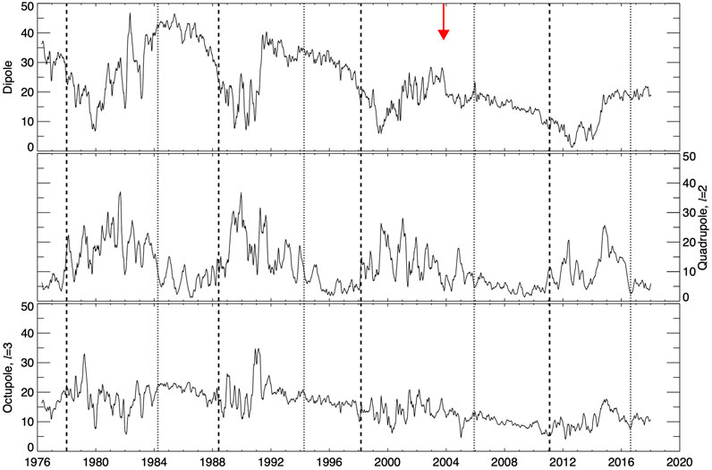
FIGURE 1. Evolution of the solar dipole and multipole components from the Wilcox Solar Observatory expansion of the coronal magnetic field. Dashed lines represent terminators; dotted lines represent the pre-terminators. The red arrow corresponds to the Halloween Storms of 2003—note the drop in dipole moment (top panel) with no parallel in any other cycle.
The top two panels of Figure 2 show the same dipole and quadrupole moment data as Figure 1, but now expressed following mSEA analysis (Chree, 1913; Leamon et al., 2021). Each of the five (partial) cycles 20–24 has its own trace in Figure 2, and the first half of the plot repeats so that the terminators, the main objects of focus, are not at the edges of the plot. Note that expressing cycle progression as a fraction of their length requires the terminator of cycle 24 to be hard-wired. For the interests of this paper it is set to December 2021, based on monthly mean F10.7 observations exceeding the F10.7 = 90 sfu threshold that is a good approximation to both the terminators and pre-terminators Chapman et al. (2020).
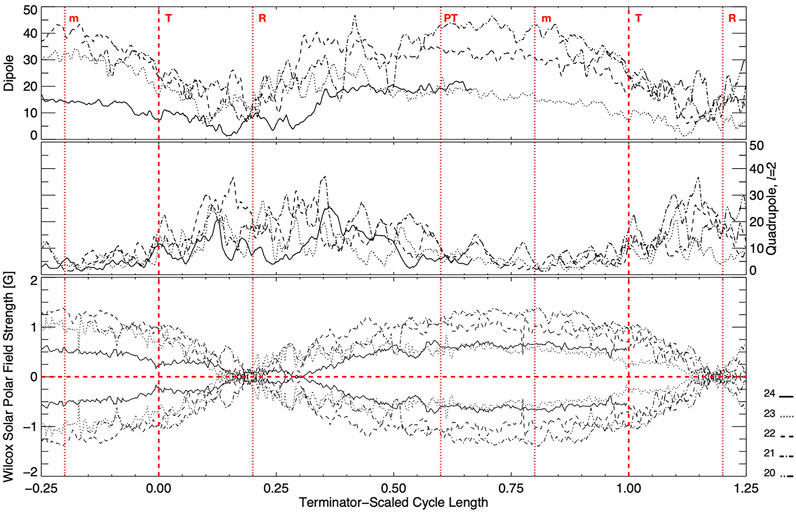
FIGURE 2. (Top, middle) Modified Superposed Epoch Analysis version of the Wilcox magnetic field expansion data of Figure 1. (bottom) Modified Superposed Epoch Analysis of the solar polar field as measured by Wilcox from 1976-present. Plotted is the average of the North and South polar apertures, (N–S)/2, and again with flipped sign. The dotted line at x = 0.2 corresponds to the polar field reversal (canonical max; labeled “R”), consistent across all five cycles; the dotted line at x = 0.8 corresponds approximately to canonical solar minimum (labeled “m”; and the dotted line at x = 0.6 corresponds to the pre-Terminator (labeled “PT”).
The mSEA analysis makes it clear to see that the terminators, represented by the dashed lines at x = 0, and the pre-terminators, represented by the dotted lines at x = 0.6, roughly bracket times with an enhanced quadrupole moment in the middle panel. The more striking result is in the other two panels: in the top panel the dipole moment has its minimum (i.e., sunspot maximum) occurring near x = 0.2. This is more clearly seen in the bottom panel of Figure 2. Rather than the Dipole field strength, here we plot the polar field strength, as measured by the Wilcox Solar Observatory (Svalgaard et al., 1978). From this mSEA we see that the polar field reversal happens almost rigidly at x = 0.2 (0.198 ± 0.013 for Cycles 21–24). We notice also the apparent symmetry of one-, three-, and four-fifths of a cycle. The dotted line at x = 0.8 (and, repeated, at x = −0.2) is the minimum of the mean quadrupole moment and represents solar activity minimum. Recall that the polar field at canonical minimum x ∼ 0.8 is used as a precursor predictor method for the upcoming cycle strength.
Chapman et al. (2020) already noticed that the first X-flare of a cycle happens close to the Terminator, and also that the pre-Terminator on the declining phase of the solar cycle ushered in the quiet interval spanning solar minimum. We shall now investigate the production of X-flares throughout the solar activity cycle. The top panel of Figure 3 shows the occurrence of all 452 X-flares in the GOES catalogue since 1976 over the trace of the (27-day smoothed) F10.7 radio flux for each solar cycle.
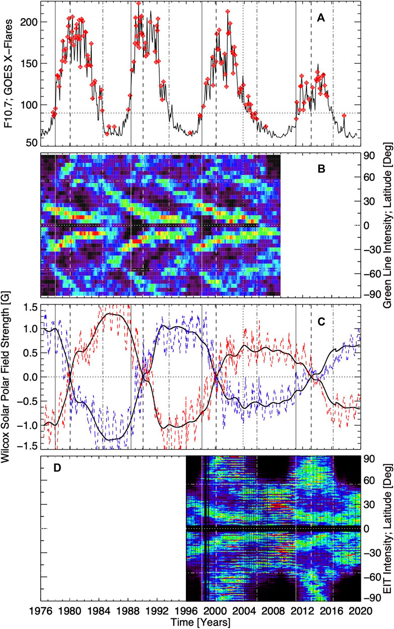
FIGURE 3. Showing the importance of the pre-Terminator across all aspects of solar output. (A) F10.7 solar radio flux, overplotted with the time of GOES X-class flares; (B) coronal Green Line emission as a function of latitude; (C) Wilcox Polar field strength, as in Figure 2 (red–south, blue–north, and the smoothed average in black); (D) EIT corona, akin to panel (B) and Figure 9 of McIntosh et al. (2014). Green Line and F10.7 data can be extended back several more decades; we limit the time axis to 1976–2020 for GOES flare and Wilcox Observatory data. Throughout all panels, terminators are marked by solid lines, the pre-Terminators (F10.7 = 90 sfu) by dot-dashed lines; solar maxima (as determined by polar field reversals in (C)) by dashed lines. The dotted vertical line corresponds to the Halloween Storms of 2003.
With large flares often occurring in close succession and the overlap of plot symbols on a 44-year plot, it might not immediately be obvious that there are 452 points in the top panel of Figure 3. In fact, the vast majority, 96%, of all X-flares happen between the Terminator and pre-Terminator; there are only 16 “contrary” X-flares in the entire record. Four of those are from AR 12673 in September 2017, and the F10.7 flux surged significantly at that epoch (when that AR was present), and exceeded the F10.7 = 90sfu threshold that is a reasonably good approximation to both the terminators and pre-terminators Chapman et al. (2020). Repeating this analysis for M-class flares, “only” 93% happen between the Terminator and pre-Terminator (only 403 out of 5,967 fall outside the range).
The second phenomenon not immediately visible in the top panel of Figure 3 is that 78% of all X-flares happen when the daily F10.7 value exceeds the 365-day trailing F10.7 average. This is probably not a surprise—the source of X-flares are large complex active regions that generate significant amounts of F10.7 emission due to their size and complexity—we’ll explore complexity more below. To further emphasize the potential “pre-requisite” nature of F10.7 for X-flares, we note that only 8 (<2%) X-flares occurred on a day with the F10.7 reading below 90 sfu, and only 13 (<3%) occurred in a Carrington rotation with the rotation average F10.7 below 90 sfu. Table 1 quantifies the number of X-flares per cycle and both of these probabilistic observations.

TABLE 1. Distribution of all 452 X-flares in the GOES catalogue, relative to the Terminators, pre-terminators and the relative levels in F10.7 radio flux.
The other three panels of Figure 3 provide context for the abrupt onset of activity at the Terminator and the abrupt turn-off of activity at the pre-Terminator. The second panel shows the off-limb (integrated from 1.15 to 1.25 solar radii) coronal Green line (Fe X IV, 5303Å) intensity as a function of latitude and time. Daily observations are smoothed with a 150-day rolling window. The overlapping activity bands of the ESC as discussed above are clearly visible. At the terminator, the old cycle bands, well, terminate. The next cycle bands are now at ∼35°. At the highest latitudes, we see the “rush to the poles” (Altrock, 1997) between the terminator and polar field reversal/solar maximum. After polar field reversal, the next cycle’s activity band starts progressing equatorward, starting from ∼55°. The fourth panel uses the same off-limb sampling process, applied to space-borne broadband EUV imagers from SOHO/EIT (195Å, 1996–2010) and SDO/AIA (193Å, 2010–) to extend the Green line observations to the present. Not unsurprisingly, the same features are seen between the Fe xiv Green line and Fe xii EUV emission. The remaining panel reprises the Solar Polar Field strength of Figures 1, 2. Through all four panels we trace vertical lines for the key landmarks of the cycle: dashed for terminators, thick dashed for polar field reversals, and dot-dashed for the pre-terminators. As in Figure 1, the Halloween storms of 2003 are marked by the single dotted vertical line. The pre-terminators occur when F10.7 ≃ 90sfu.
Figure 4 re-expresses the data of Figure 3 in the form of the modified superposed epoch analysis, akin to Figures 1, 2. We omit the EIT/AIA EUV data as it barely covers two solar activity cycles. Instead it is replaced by the Calcium ii K record of cycles 14–20 (∼1913–1977) from the Kodaikanal Observatory, as compiled by Chatterjee et al. (2019). Combined, Figures 3, 4 bring many things into focus. We notice that, at the terminator, there is no more old cycle flux activity bands at the equator, further the new cycle bands at mid-latitudes activate, and we observe an increase in coronal emission and in flaring. Note also at high latitudes we observe the rush to the poles (McIntosh et al., 2019).
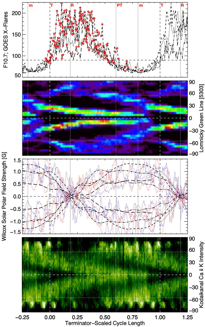
FIGURE 4. Modified Superposed Epoch Analysis version of Figure 3. The EIT panel is replaced by the Calcium ii K record of cycles 14–20 (∼1913–1977) from the Kodaikanal Observatory. The labels “T,” “R,” “PT,” and “m” are the same as from Figure 2.
One-fifth of a cycle later, we observe the polar field reversal. Two-fifths of a cycle later again, at the pre-terminator, the new (i.e., next) cycle bands starts moving equatorward at 55° (as seen in the EIT, Green Line and Calcium ii K intensity panels), and the current cycle bands are at about 15° latitude. Independent of the actual mechanism of “quenching,” the presence of four (two, of opposite polarity, in each hemisphere) bands on the disk leads to high-energy flaring activity to abruptly reduce to almost zero.
We surmise that the turn-off in activity at the pre-terminator is due to a (sudden) decrease in active region complexity. Jaeggli and Norton (2016) noted that “there are no published results showing the variation of the Mount Wilson magnetic classifications as a function of solar cycle” and, as an attempted rectification, considered the fraction of complex (γ and/or δ) sunspot groups from 1992 to 2015, albeit only on an annually-averaged basis. They did find a sharp decrease in the number of the most complex βγδ regions prior to minima in 1995 and 2007, and increase in the fraction of simple α regions, but the direct utility to our study is limited due to the annual averaging applied. Similarly, McAteer et al. (2005) considered the fractal dimension of a 50 Gauss threshold contour of all ARs seen by SOHO/MDI from 1996 to 2004, but focused more on testing a correlation of active region complexity to flare likelihood, but unfortunately, curtailed their study before the Cycle 23 pre-terminator.
In the absence, then, of a complete database of active region classifications, we can consider the distribution of spot areas from the Greenwich/USAF record as proxy, which is what is shown in Figure 5. The three panels are the mean, skewness and excess kurtosis of the spot areas on a (Carrington) rotation-by-rotation basis. There are clear Terminator and pre-terminator signals, especially in the higher order moments. (Recall excess kurtosis has three subtracted from the moment calculation, as three is the computed value of a Gaussian distribution. Thus excess kurtosis <0 means flatter than Gaussian; similarly, skewness >0 means the distribution is skewed to the right, with a longer tail to the right of the distribution maximum.) Overlaying the kurtosis panel of Figure 5 for the last half of the record is F10.7. The correspondence between kurtosis, and F10.7, simply scaled and shifted, especially from ∼1960 (post Cycle-19 maximum) on, is quite remarkable. F10.7 can be considered as just an integrated measure of global complexity of the solar magnetic field.
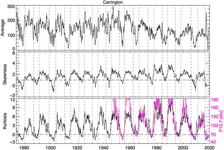
FIGURE 5. The complexity of sunspots changes at Terminators and Pre-Terminators. As a proxy of geometric complexity for individual spots, we compute the moments of the distribution of spot area from the Greenwich/USAF archive. From the top, the three panels are the average, skewness and excess (compared to a Gaussian) kurtosis. Dashed vertical lines indicate the Terminators in red, Pre-Terminators in blue. The kurtosis is a more than reasonable proxy for the F10.7 radio flux.
We complete our description of the Hale Cycle with one further analysis of the F10.7 radio flux. The top panel of Figure 6 again shows the complete 1947–present record of F10.7, with the Terminators and pre-terminators marked as vertical dashed red lines. Here we add markers of 0.2 cycle and 0.4 cycle as vertical dotted lines. In all cycles, and markedly so in Cycles 20 and 22, there is a distinct drop-off from its maximum (solar maximum) value at around 0.4 cycles. To investigate this further, we compute a unit cycle, following the methods of Leamon et al. (2021).
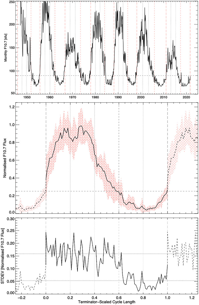
FIGURE 6. (Top) The complete F10.7 record, with 0.2, 0.4, and 0.6 of a cycle indicated by vertical lines. (middle) The terminator-terminator Unit Cycle, scaled to each cycle’s maximum radio flux, as computed from the above. The rapid surge in F10.7 at the Terminator, dip around polar field reversal at 0.2 cycles, and sharp drop at 0.4 cycles (when elements of the next cycle appear at high latitudes) are all clearly visible. The red envelope marks the standard deviation for each 0.01-cycle step. (bottom) The standard deviation from the middle panel plotted alone. Note the step change at the Terminator and pre-terminator (closer to 0.62 cycles by this measure). The horizontal dotted lines indicate the means before and after the pre-terminator.
To create the middle panel of Figure 6, we take the almost seven cycles of F10.7 data from the top panel, subtract off the minimum value of 65.0 sfu, and scale each cycle to the maximum of its (13-month smoothed) record. We then scale time as a fraction of Terminator-Terminator time, interpolated to 100 points, and plot the mean and standard deviation for each fractional time (thick black line and red hatched envelope; the thickness of the latter is reproduced as in the bottom panel). There is consistently:
1. at the Terminator, a rapid surge in F10.7 (through 90 sfu, almost by definition);
2. at 0.2 cycles, a dip around polar field reversal;
3. at 0.4 cycles, a sharp drop—when the polar coronal hole and polar crown filament reform and elements of the next cycle appear at high latitudes;
4. at 0.6 cycles, the onset of “quiet” conditions with greatly reduced numbers of X-flares as discussed before, and with approximately the same F10.7 output as at the Terminator;
5. at 0.8 cycles, approximately canonical minimum, the pattern completes.
The bottom panel of Figure 6 further shows that there is also a clear change in the standard deviation (thickness of red envelope), at the Terminator and ∼0.6 cycles. The local minimum at ∼0.4–0.5 cycles (lasting longer than the other, spikier, changes earlier in the cycle) may also be significant. Regardless of the strength of the cycle or whatever short term activity surges are superimposed on it, the nature of (the complexity of) sunspots changes at these landmarks of the 22-year Hale Magnetic Cycle.
Finally, for an approximately 11-year cycle, we note there are approximately 150 Carrington rotations per cycle, so each fifth, or phase, or “season” of the solar activity cycle takes approximately 30 rotations.
We have shown that the Sun’s rate of energetic flare production, geomagnetic storm activity, and active region complexity all surge simultaneously at the termination of Hale Cycles—when there is no more old cycle polarity flux left on the disk. Similarly, and independent of the strength or length of the solar cycle, these measures decrease in concert at approximately 3/5 of the duration of the cycle; again these observations are tied to the behavior of the flux systems belonging to the two overlapping Hale Cycles present on (or, well, in) the Sun.
It is not a new finding that the new 11-year activity cycle turns on rapidly at mid-latitudes. But it is precisely the unfettering of the new cycle’s bands following the termination of the old cycle bands at the equator, that permits a systematic increase in magnetic flux emergence across many longitudes to occur at mid-latitudes through the growth of sunspot groups, and at high latitudes with the onset of the “rush to the poles.”
Our efforts thus far have focused on discrete magnetic elements (sunspots, brightpoints, and filaments) and resolvable emission (maps of the Fe xiv Green line coronal off-limb and Calcium ii K on-disk. Put another way, we have focused on the small-scale tracers of the large-scale motions of the magnetized solar plasma that comprise the Hale Cycle. We now focus on large-scale tracers: sun-as-a-star measures of coronal emission.
McIntosh et al. (2019) and Leamon et al. (2021) demonstrated that there was a significant surge in EUV spectral irradiance across the cycle 23 terminator, on a timescale of less than a solar rotation, and possibly as little as a week. The Leamon et al. (2021) results from SDO/EVE, considering the irradiance of the various AIA EUV lines, is reproduced as panel (A) of Figure 7. From bottom to top, the lines increase in their formation temperature. Each successively hotter line is scaled to the time interval 180–60 days prior to the pre-terminator, and offset on the y-axis by unity, except for the hottest line—Fe xvi 335Å—which is offset by two to show the largest change: a ∼180% increase in Fe xvi 335Å emission across the terminator. Due to the failure of the SDO/EVE MEGS-A sensor in May 2014, a direct comparison to the 2016 pre-terminator is not possible. However, a partial comparison can be made using EVE’s single-band diodes for 304Å, 171Å, 335Å, and Lyman-α (1216Å), and is shown in the panel (B) of Figure 7. The rapid change is demonstrated by the dashed vertical line of the pre-terminator, as determined by the analyses in Section 2, and the dotted vertical line that corresponds to one Carrington Rotation later. The pre-post ratios are, respectively: Lyman = 0.93; 304Å = 0.94; 171Å = 0.88; 335Å = 0.51.
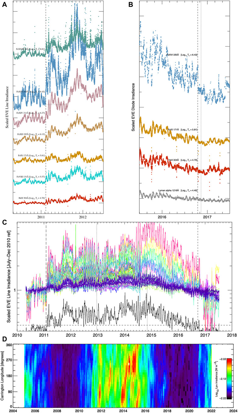
FIGURE 7. (A), (B), (C) Scaled SDO/EVE irradiances as functions of time. (D) Lyman-α as a function of time and Carrington Longitude. See text, Section 3.1, for more details.
The strongest response is seen in Fe XVI 335Å, which shows a factor of ∼2 change over the course of one solar rotation at both the Terminator and pre-terminator. Lyman-α shows ∼6% change at both times too; smaller change amplified by sheer number of photons—Lyman-α is the most intense line of the solar spectrum at 0.007 W m − 2 nm − 1 at minimum, rising to 0.009 W m − 2 nm − 1 at the peak of C24 or similar weak cycles, or 0.01 W m − 2 nm − 1 at the peak of relatively strong cycles (Lemaire et al., 2015; Kretzschmar et al., 2018). Thus a 6% change at the terminator (and pre-terminator) represents approximately one quarter of the entire min-to-max cycle variation, and thus has significant ionospheric and upper atmosphere impact (Chandra and McPeters, 1994; Lean, 2000; Leamon et al., 2021).
These step changes in radiative output occur independent of wavelength. To illustrate this, panel (C) of Figure 7 shows the simultaneous onset and cessation of all (hot) coronal lines from SDO/EVE, covering the whole interval from the start of panel (A) to the end of panel (B).1 For reference, the black trace is F10.7, similarly scaled to its July–December 2010 average, and displaced down by a factor of 3, and the dashed horizontal line corresponding to 90 sfu. The simultaneous onset of enhanced emission in all hot coronal lines at the terminator in February 2011, and its cessation in August 2016, are clear. We reiterate that this step change in radiative output occurs independent of wavelength, and is co-temporal with the drop-off in high energy flares.
Finally, panel (D) of Figure 7 synthesizes the longitudinal evolution of Lyman-α emission as a function of Carrington Longitude and time from 2005–present. (This panel is an extension of Figure 3A of Leamon et al. (2021), and panels (C) and (D) are not a stack plot—note the different time axis scales between them. Again, the onset of enhanced emission at the terminator and its cessation at the pre-terminator, are clear—and global. There are preferred longitudes (i.e., active regions; red colors) at the SSN peak in 2014, but the transition from blue–green in 2011 and then from green–blue in 2016 are independent of longitude. As panels (A) and (B) showed, the change from “hot corona” to “warm corona” (Schonfeld et al., 2017) happens over a single rotation.
EUV Photons emitted from hot coronal plasma and energetic flares both require significant energy to be supplied to the corona from below. Why does the energy available for coronal energetics rise so sharply and dramatically fall when F10.7 ≃ 90 sfu? At the pre-terminator, the new (i.e., next) cycle bands starts moving equatorward from 55° (as seen in the EIT, Green Line and Calcium ii K intensity panels), and the current cycle bands are at about 15° latitude. Two possibilities that explain the decrease in activity related to band location are:
• being 30° apart means greater interaction between the two current-cycle bands across the equator, reducing energy available for coronal energetics (e.g., Dikpati et al., 2021); or
• being at or below some critical latitude means that the north-south shear from differential rotation is too great to support or maintain large complex ARs, reducing energy available for coronal energetics (Spruit, 2011).
Independent of the actual mechanism of “quenching,” the presence of four (two, of opposite polarity, in each hemisphere) bands on the disk, each separated by ∼30°, at the pre-terminator leads to less complex magnetic field configurations, which in turn abruptly reduce high-energy flaring activity to almost zero. Simultaneously, spectral emission from the hot corona falls off just as abruptly, and the F10.7 solar radio flux—which again can be considered as just an integrated measure of global complexity of the solar magnetic field—returns to the 90 sfu level it had at the Terminator 0.6 cycles (∼6–7 years) previously.
Since the flux system that is now providing cycle 25 activity has been present on the Sun since just after the cycle 24 solar maximum (see, e.g., Figure 1 of Leamon et al., 2020), we can already predict when cycle 25 will end by linear extrapolation of the cycle 25 bands’ equatorward progress. Leamon et al. (2020) thus determined October 2031 ± 9 months, which puts the cessation of major solar activity associated with the next pre-terminator in the first half of 2027 (March ±6 months).
These predictions will be refined at the polar field reversal (one-fifth of the way through the terminator-to-terminator cycle)—which we may currently estimate to be the first half of 2024. We note that according to the recent results of Owens et al. (2021), the likelihood of extreme geomagnetic consequences among those events that do occur in ∼2024–2027 after the polar field reversal and before the pre-terminator is increased compared to the coming few years (the rise phase of the cycle from now until the polar field reversal). For reference, Solar Orbiter’s fifth Venus Gravity Assist maneuver will occur in December 2026, lifting the peak heliolatitude of its orbit to ∼25° in March 2027, which is extremely fortuitous timing to observe the anticipated pre-Terminator changes in flux systems at 55°. Two other out-of-ecliptic missions are under consideration by NASA—the Solar Cruiser Mission-of-Opportunity is in development (to launch with IMAP, scheduled for early 2025), and the Solaris concept is in a Phase-A study for the next MIDEX mission, and if selected will launch in late 2025 and will make its first high-latitude polar pass in mid 2029.
The significant advances these coming observations will make, together with the decade of step-by-step improvements to theory and modeling (constrained by said significant observational advances) they will drive, makes it probable that, as it rises through 2022, Cycle 25 will be the last solar activity cycle that is not fully understood.
We have previously shown the concept of Hale Cycle Terminators (end of the 22-year Hale Magnetic Cycle) producing rapid changes in solar activity in a year or two after the canonical solar minimum. Here we have demonstrated, through combined observations of the Sun’s radiative, particulate and ejecta output, that there does appear to be a Solar Clock defined by the Terminators of each Hale Magnetic Cycle that can explain changes in solar activity in the 11-or-so years between Terminators. Landmarks of this clock, such as the first and last X-class flare, F10.7 exceeding and falling below a certain threshold, the poleward motion of the highest latitude filaments, and the reversal of the polar field all appear to occur at fixed points in this (unit) cycle.
The repeating global-scale magnetic pattern that first appears at ∼55° latitude, with one branch rushing to the poles over 2–3 years and the second progressing equatorward over 19–20 years, is key to understanding the ESC, which is the Hale Magnetic cycle. Other than the rush-to-the-poles time, there are four oppositely signed magnetic bands between 55° and the equator, and their interactions drive solar activity.
On a clock that goes from Terminator to Terminator, there are five clear landmarks, equally distributed in phase: The terminator, originally defined in terms of the distribution of EUV brightpoints on the disk, is also well approximated by the F10.7 solar radio flux exceeding 90 sfu, the first X-class flare of the cycle, a step increase in EUV emission from the million-degree corona, and the rush to the poles of polar crown filaments, closing the polar coronal hole. The reversal of the polar fields occurs at 0.2 cycles. The polar crown filaments and polar coronal holes have reformed at 0.4 cycles, and there is a clear and sudden drop in active region complexity and F10.7 (just as there was the surge in activity at the Terminator with the rush to the poles). At 0.6 cycles, aka “pre-Terminator,” the F10.7 index again is 90 sfu, the same as at the terminator; simultaneously there is a significant and simultaneous reduction in EUV emission (factor ∼2 in 335Å) and X-flare production. Indeed, only 16/453 X-flares observed by GOES are deviant in occurring outside the “core” 60% of the solar cycle, and the pre-Terminator can be considered the “onset of solar minimum conditions.”
Comparisons of stellar radiative flux and magnetic flux have resulted in strong correlations and scaling laws with X-ray flux (Pevtsov et al., 2003) and XUV flux (Vidotto et al., 2014). Replicating the latter’s techniques with Sun-as-a-star measurements, Hazra et al. (2020) showed a strong correlation (r ∼ 0.99) between the integrated XUV spectrum and the solar magnetic flux. Figure 5 of Hazra et al. (2020) is particularly insightful as it pertains to our arguments here; the azimuthally-averaged radial magnetic flux shows a sharp rise in 2011 (at the Cycle 23 Terminator), and drop at the end of 2014 (at the 0.4 cycle mark of Cycle 24), corresponding to the period when there is not a coherent polar coronal hole or polar crown filament. It is the distribution of magnetic elements across the (4π) solar surface that matters, not just their scalar strength or vector orientation.
From extrapolating observations of the distribution of EUV brightpoints we can already estimate that the Cycle 25 Terminator will be late 2031—early 2032. Thus, we may estimate that the pre-Terminator, and last X-flare of Cycle 25 will occur in mid-2027 (approximately the time of the first Solar Orbiter high latitude pass). Since we know that polar field reversal occurs at 0.2 cycles, we can confirm, refine, or revise our estimate for the length of Cycle 25 as early as its polar field reversal, which we currently estimate to be early-mid 2024.
In closing, in light of the theme of this Frontiers Research Topic, “Short- and Long-Term Solar Activity and its Potential Influences on Earth’s Atmosphere,” we have shown that there are rapid changes in the number of energetic photons (both X-rays from flares, and EUV emission from the hot corona) impinging on the atmosphere at specific times in the cycle. These times are predictable. As such, the results presented here suggest that solar (cycle-modulated) inputs are not properly captured in current atmospheric models, and thus we offer great utility for improving the fidelity of atmospheric and climate modelling in future.
This study uses a wide range of solar remote observations, from both space-borne satellites and ground-based observatories. All datasets analyzed for this study can be found in their linked repositories, as explained below.
From space, the primary motivator of all activity bands studies is the determination and tracking of EUV BPs from The Solar and Heliospheric Observatory (SOHO) Extreme-ultraviolet Imaging Telescope (EIT) (Delaboudinière et al., 1995) and Solar Dynamics Observatory (SDO) Atmsopheric Imaging Assembly (AIA) (Lemen et al., 2012) telescopes (in 195Å and 193Å, respectively). Following McIntosh et al. (2014), we identify BPs in a manner that accounts for differences in the two instruments. SDO also provides spectral irradiance data via the EUV Variability Experiment (EVE) (Woods et al., 2012). The other space-based dataset used is the Geostationary Operational Environmental Satellites (GOES) X-ray flare catalog2 combining measurements from the series of 17 GOES satellites from 1976–present (Chamberlin et al., 2009).
From the ground, the Wilcox Solar Observatory3 (Scherrer et al., 1977) provides solar magnetic field measurements (also 1976–present). We also use longer-term synoptic ground-based solar observations, including the Penticton 10.7 cm radio flux4 (Tapping, 2013); and the NGDC composite Coronal Green Line (Fe xiv) data5 (Rybansky et al., 1994). sunspot number data is from the Solar Information Data Center (SIDC; SILSO World Data Center, 1960–2020; Vanlommel et al., 2005), and sunspot area from the combined Royal Greenwich Observatory/United States Air Force record, originally compiled and maintained by NASA’s Marshall Space Flight Center6 (Hathaway, 2015).
RL and SM conceived the experiment and analyzed the results. RL wrote the original draft; SM and RL led reviewing and editing. RL created all figures. AT contributed discussions to the sections on flare production. All authors reviewed the manuscript.
RL is supported by NASA’s Living With a Star Program. SM is supported by the National Center for Atmospheric Research, which is a major facility sponsored by the National Science Foundation under Cooperative Agreement No. 1852977. RL also appreciates the support of NCAR’s HAO Visitor Program, which enabled discussions with SM.
Author AT was employed by Lockheed Martin Corporation.
The remaining authors declare that the research was conducted in the absence of any commercial or financial relationships that could be construed as a potential conflict of interest.
All claims expressed in this article are solely those of the authors and do not necessarily represent those of their affiliated organizations, or those of the publisher, the editors and the reviewers. Any product that may be evaluated in this article, or claim that may be made by its manufacturer, is not guaranteed or endorsed by the publisher.
We thank Sandra Chapman and Nicholas Watkins for discussions improving earlier versions of this manuscript. We thank Phil Scherrer and J.∼Todd Hoeksema for their assistance with, and discussions on, the Wilcox Solar Observatory data, and Dipankar Bannerjee and Subhamoy Chatterjee for their assistance with the Kodaikanal Observatory data. Finally, we acknowledge the numerous contributions to Solar Physics of the late Eugene N. Parker (1927-2022); not just the bold prediction of the supersonic solar wind, but also, relevant to this work, the dynamo, the hot corona, and the Martial Art of Scientific Publication.
1The 12 lines with wavelengths below 330Å only have data up to the May 2014 MEGS-A anomaly; but all 39 lines show the same surges in intensity on both 27-day and 6–9 month timescales up to that unfortunate date, and all lines above 330Å show the simultaneous cessation in August 2016.
2www.ngdc.noaa.gov/stp/space-weather/solar-data/solar-features/solar-flares/x-rays/goes/xrs/.
3wso.stanford.edu/HCS.html.
4spaceweather.gc.ca/solarflux/sx-4-en.php.
5www.ngdc.noaa.gov/stp/solar/corona.html.
6solarscience.msfc.nasa.gov/greenwch.shtml.
Altrock, R. C. (1997). An ‘Extended Solar Cycle’ as Observed in Fe XIV. Sol. Phys. 170, 411–423. doi:10.1023/a:1004958900477
Arlt, R. (2008). Digitization of Sunspot Drawings by Staudacher in 1749 - 1796. Sol. Phys. 247, 399–410. doi:10.1007/s11207-007-9113-4
Babcock, H. W. (1961). The Topology of the Sun's Magnetic Field and the 22-YEAR Cycle. Astrophys. J. 133, 572. doi:10.1086/147060
Biesecker, D. A., and Upton, L. (2019). Solar Cycle 25 Consensus Prediction Update. AGU Fall Meet. Abstr. 2019, SH13B–03.
Chamberlin, P. C., Woods, T. N., Eparvier, F. G., and Jones, A. R. (2009). “Next Generation X-ray Sensor (XRS) for the NOAA GOES-R Satellite Series,” in Solar Physics and Space Weather Instrumentation III (San Diego, California: Proceedings of the SPIE), 743802. doi:10.1117/12.826807
Chandra, S., and McPeters, R. D. (1994). The Solar Cycle Variation of Ozone in the Stratosphere Inferred from Nimbus 7 and NOAA 11 Satellites. J. Geophys. Res. 99, 20665–20671. doi:10.1029/94JD02010
Chapman, S. C., McIntosh, S. W., Leamon, R. J., and Watkins, N. W. (2020). Quantifying the Solar Cycle Modulation of Extreme Space Weather. Geophys. Res. Lett. 47. doi:10.1029/2020GL087795
Chatterjee, S., Banerjee, D., McIntosh, S. W., Leamon, R. J., Dikpati, M., Srivastava, A. K., et al. (2019). Signature of Extended Solar Cycles as Detected from Ca II K Synoptic Maps of Kodaikanal and Mount Wilson Observatory. Astrophys. J. Lett. 874, L4. doi:10.3847/2041-8213/ab0e0e
Chree, C. (1913). III. Some Phenomena of Sunspots and of Terrestrial Magnetism at Kew Observatory. Phil. Trans. R. Soc. Lond. A. 212, 75–116. doi:10.1098/rsta.1913.0003
Delaboudinière, J.-P., Artzner, G. E., Brunaud, J., Gabriel, A. H., Hochedez, J. F., Millier, F., et al. (1995). EIT: Extreme-Ultraviolet Imaging Telescope for the SOHO Mission. Sol. Phys. 162, 291–312. doi:10.1007/978-94-009-0191-9_8
Dicke, R. H. (1978). Is There a Chronometer Hidden Deep in the Sun? Nature 276, 676–680. doi:10.1038/276676b0
Dikpati, M., McIntosh, S. W., Chatterjee, S., Norton, A. A., Ambroz, P., Gilman, P. A., et al. (2021). Deciphering the Deep Origin of Active Regions via Analysis of Magnetograms. Astrophys. J. 910, 91. doi:10.3847/1538-4357/abe043
Hale, G. E., Ellerman, F., Nicholson, S. B., and Joy, A. H. (1919). The Magnetic Polarity of Sun-Spots. Astrophys. J. 49, 153. doi:10.1086/142452
Harvey, K. L. (1992). “The Cyclic Behavior of Solar Activity,” in The Solar Cycle; Proceedings of the National Solar Observatory/Sacramento Peak 12th Summer Workshop, ASP Conference Series (San Francisco: ASP), 335.
Hazra, G., Vidotto, A. A., and D’Angelo, C. V. (2020). Influence of the Sun-like Magnetic Cycle on Exoplanetary Atmospheric Escape. Mon. Not. Roy. Astron. Soc. 496, 4017–4031. doi:10.1093/mnras/staa1815
Hoyng, P. (1996). Is the Solar Cycle Timed by a Clock? Sol. Phys. 169, 253–264. doi:10.1007/BF00190603
Jaeggli, S. A., and Norton, A. A. (2016). The Magnetic Classification of Solar Active Regions 1992-2015. Astrophys. J. 820, L11. doi:10.3847/2041-8205/820/1/L11
Joselyn, J. A., Anderson, J. B., Coffey, H., Harvey, K., Hathaway, D., Heckman, G., et al. (1997). Panel Achieves Consensus Prediction of Solar Cycle 23. Eos Trans. AGU 78, 205. doi:10.1029/97EO00136
Kretzschmar, M., Snow, M., and Curdt, W. (2018). An Empirical Model of the Variation of the Solar Lyman‐ α Spectral Irradiance. Geophys. Res. Lett. 45, 2138–2144. doi:10.1002/2017GL076318
Leamon, R. J., McIntosh, S. W., Chapman, S. C., and Watkins, N. W. (2020). Timing Terminators: Forecasting Sunspot Cycle 25 Onset. Sol. Phys. 295, 36. doi:10.1007/s11207-020-1595-3
Leamon, R. J., McIntosh, S. W., and Marsh, D. R. (2021). Termination of Solar Cycles and Correlated Tropospheric Variability. Earth Space Sci. 8, e01223. doi:10.1029/2020EA001223
Lean, J. (2000). Evolution of the Sun's Spectral Irradiance since the Maunder Minimum. Geophys. Res. Lett. 27, 2425–2428. doi:10.1029/2000GL000043
Leighton, R. B. (1969). A Magneto-Kinematic Model of the Solar Cycle. Astrophys. J. 156, 1. doi:10.1086/149943
Lemaire, P., Vial, J.-C., Curdt, W., Schühle, U., and Wilhelm, K. (2015). Hydrogen Ly-Αand Ly-Βfull Sun Line Profiles Observed with SUMER/SOHO (1996-2009). Astron. Astrophys. 581, A26. doi:10.1051/0004-6361/201526059
Lemen, J. R., Title, A. M., Akin, D. J., Boerner, P. F., Chou, C., Drake, J. F., et al. (2012). The Atmospheric Imaging Assembly (AIA) on the Solar Dynamics Observatory (SDO). Sol. Phys. 275, 17–40. doi:10.1007/s11207-011-9776-8
Leroy, J. L., and Noens, J. C. (1983). Does the Solar Activity Cycle Extend over More Than an 11-year Period? Astron. Astrophys. 120, L1.
McAteer, R. T. J., Gallagher, P. T., and Ireland, J. (2005). Statistics of Active Region Complexity: A Large‐Scale Fractal Dimension Survey. Astrophys. J. 631, 628–635. doi:10.1086/432412
McIntosh, S. W., Chapman, S., Leamon, R. J., Egeland, R., and Watkins, N. W. (2020). Overlapping Magnetic Activity Cycles and the Sunspot Number: Forecasting Sunspot Cycle 25 Amplitude. Sol. Phys. 295, 163. doi:10.1007/s11207-020-01723-y
McIntosh, S. W., Leamon, R. J., Egeland, R., Dikpati, M., Altrock, R. C., Banerjee, D., et al. (2021). Deciphering Solar Magnetic Activity: 140 Years of the 'Extended Solar Cycle' - Mapping the Hale Cycle. Sol. Phys. 296, 189. doi:10.1007/s11207-021-01938-7
McIntosh, S. W., Leamon, R. J., Egeland, R., Dikpati, M., Fan, Y., and Rempel, M. (2019). What the Sudden Death of Solar Cycles Can Tell Us about the Nature of the Solar interior. Sol. Phys. 294, 88. doi:10.1007/s11207-019-1474-y
McIntosh, S. W., Wang, X., Leamon, R. J., Davey, A. R., Howe, R., Krista, L. D., et al. (2014). Deciphering Solar Magnetic Activity. I. On the Relationship between the Sunspot Cycle and the Evolution of Small Magnetic Features. Astrophys. J. 792, 12. doi:10.1088/0004-637X/792/1/12
Owens, M. J., Lockwood, M., Barnard, L. A., Scott, C. J., Haines, C., and Macneil, A. (2021). Extreme Space-Weather Events and the Solar Cycle. Sol. Phys. 296, 82. doi:10.1007/s11207-021-01831-3
Pesnell, W. D. (2008). Predictions of Solar Cycle 24. Sol. Phys. 252, 209–220. doi:10.1007/s11207-008-9252-2
Pevtsov, A. A., Fisher, G. H., Acton, L. W., Longcope, D. W., Johns‐Krull, C. M., Kankelborg, C. C., et al. (2003). The Relationship between X‐Ray Radiance and Magnetic Flux. Astrophys. J. 598, 1387–1391. doi:10.1086/378944
Russell, C. T., Jian, L. K., and Luhmann, J. G. (2019). The Solar Clock. Rev. Geophys. 57, 1129–1145. doi:10.1029/2019RG000645
Rybanský, M., Rušin, V., Minarovjech, M., and Gašpar, P. (1994). Coronal index of Solar Activity: Years 1939-1963. Sol. Phys. 152, 153–159. doi:10.1007/BF01473198
Schatten, K. H., Wilcox, J. M., and Ness, N. F. (1969). A Model of Interplanetary and Coronal Magnetic fields. Sol. Phys. 6, 442–455. doi:10.1007/BF00146478
Scherrer, P. H., Wilcox, J. M., Svalgaard, L., Duvall, T. L. , Dittmer, P. H., and Gustafson, E. K. (1977). The Mean Magnetic Field of the Sun: Observations at Stanford. Sol. Phys. 54, 353–361. doi:10.1007/BF00159925
Schonfeld, S. J., White, S. M., Hock-Mysliwiec, R. A., and McAteer, R. T. J. (2017). The Slowly Varying Corona. I. Daily Differential Emission Measure Distributions Derived from EVE Spectra. Astrophys. J. 844, 163. doi:10.3847/1538-4357/aa7b35
Schwabe, H. (1844). Sonnenbeobachtungen im Jahre 1843. Von Herrn Hofrath Schwabe in Dessau. Astronomische Nachrichten 21, 233. doi:10.1002/asna.18440211505
SILSO World Data Center (1960–2020). “The International Sunspot Number,” in International Sunspot Number Monthly Bulletin and Online Catalogue (Springer).
Spruit, H. C. (2011). “Theories of the Solar Cycle: A Critical View,” in The Sun, the Solar Wind, and the Heliosphere. Editors M. P., Miralles and J. Sánchez Almeida (Springer), 39–49. doi:10.1007/978-90-481-9787-3_5
Svalgaard, L., Duvall, T. L., and Scherrer, P. H. (1978). The Strength of the Sun's Polar fields. Sol. Phys. 58, 225–239. doi:10.1007/BF00157268
Tapping, K. F. (2013). The 10.7 Cm Solar Radio Flux (F10.7). Space Weather 11, 394–406. doi:10.1002/swe.20064
Vanlommel, P., Cugnon, P., Linden, R. A. M. V. D., Berghmans, D., and Clette, F. (2004). The SIDC: World Data center for the sunspot index. Sol. Phys. 224, 113–120. doi:10.1007/s11207-005-6504-2
Vidotto, A. A., Gregory, S. G., Jardine, M., Donati, J. F., Petit, P., Morin, J., et al. (2014). Stellar Magnetism: Empirical Trends with Age and Rotation. Mon. Not. Roy. Astron. Soc. 441, 2361–2374. doi:10.1093/mnras/stu728
Wilson, P. R., Altrocki, R. C., Harvey, K. L., Martin, S. F., and Snodgrass, H. B. (1988). The Extended Solar Activity Cycle. Nature 333, 748–750. doi:10.1038/333748a0
Wolf, R. (1861). Abstract of His Latest Results. Monthly Notices R. Astronomical Soc. 21, 77–78. doi:10.1093/mnras/21.3.77
Woods, T. N., Eparvier, F. G., Hock, R., Jones, A. R., Woodraska, D., Judge, D., et al. (2012). Extreme Ultraviolet Variability Experiment (EVE) on the Solar Dynamics Observatory (SDO): Overview of Science Objectives, Instrument Design, Data Products, and Model Developments. Sol. Phys. 275, 115–143. doi:10.1007/s11207-009-9487-6
Keywords: Solar activity cycle, Flares, Corona, Magnetic fields, Radio emissions, Ultraviolet emissions
Citation: Leamon RJ, McIntosh SW and Title AM (2022) Deciphering Solar Magnetic Activity: The Solar Cycle Clock. Front. Astron. Space Sci. 9:886670. doi: 10.3389/fspas.2022.886670
Received: 28 February 2022; Accepted: 07 April 2022;
Published: 10 May 2022.
Edited by:
Fadil Inceoglu, National Centers for Environmental Information (NCEI) at National Atmospheric and Oceonographic Administration (NOAA), United StatesReviewed by:
Gopal Hazra, Leiden University, NetherlandsCopyright © 2022 Leamon, McIntosh and Title. This is an open-access article distributed under the terms of the Creative Commons Attribution License (CC BY). The use, distribution or reproduction in other forums is permitted, provided the original author(s) and the copyright owner(s) are credited and that the original publication in this journal is cited, in accordance with accepted academic practice. No use, distribution or reproduction is permitted which does not comply with these terms.
*Correspondence: Robert J. Leamon, cm9iZXJ0LmoubGVhbW9uQG5hc2EuZ292
Disclaimer: All claims expressed in this article are solely those of the authors and do not necessarily represent those of their affiliated organizations, or those of the publisher, the editors and the reviewers. Any product that may be evaluated in this article or claim that may be made by its manufacturer is not guaranteed or endorsed by the publisher.
Research integrity at Frontiers
Learn more about the work of our research integrity team to safeguard the quality of each article we publish.