 Steve B. Howell
 Elise Furlan
- 1NASA Ames Research Center, Moffett Field, CA, United States
- 2NASA Exoplanet Science Institute, Caltech/IPAC, Pasadena, CA, United States
Using 3 years of observations with the Zorro and ’Alopeke speckle interferometric instruments at Gemini South and North, respectively, we present an analysis of the sensitivity of the data taken in two narrow-band optical filters centered at 562 and 832 nm (widths of 54 and 40 nm, respectively). In this paper we focus on model calculations of the predicted signal-to-noise values achievable and the results of over 2500 actual observations. We find that S/N values of several 100 are easily achieved, but that the sky background during full moon is a very limiting factor in the observations, especially those performed in the short-wavelength (blue) optical spectral range and for targets fainter than R ∼14. A comparison of our Gemini speckle observations over six observing semesters reveals that red band-pass observations provide more robust results in general, likely due to better atmospheric performance at these wavelengths. Using the identical instruments on Gemini North and South, we find that similar results are obtained, yielding typical contrast limits of 5-9 magnitudes from the diffraction limit out to 1.2″ for a range of target brightness (optical magnitudes from ∼ 3 to
1 Speckle Interferometry at Gemini
Two identical instruments have been built and deployed at the twin Gemini 8-m telescopes in Hawaii and Chile. Named ’Alopeke and Zorro (at Gemini North and South, respectively), these instruments specialize in speckle interferometric imaging1, a technique that obtains high-resolution optical images using fast exposure times and Fourier analysis techniques. The exposure times are selected in order to approximate the coherence time of the atmosphere as well as the anticipated size of a typical seeing cell (Fried, 1966). Coherence times and seeing cell size depend on the wavelength of observation (they vary from 100 ms in the infrared to 10 ms at the atmospheric cutoff in the blue), the altitude of the observatory, and the telescope diameter. Horch et al. (2011, 2012) used empirical observations over the range of 30–80 ms to show that the “Fried” model atmospheric calculations yield typical average values for speckle integration times of 60 ms at Gemini. Speckle imaging yields angular resolutions that reach the diffraction limit across the optical band-pass. The Gemini 8-m telescopes and their mountain sites are designed to deliver very good native seeing, typically less than 0.8″ and often better than 0.5″. Having such good native seeing feeding the speckle instruments allows high S/N, diffraction-limited (20–30 mas) high-resolution imagery to be possible.
The ’Alopeke and Zorro instruments (Scott et al., 2021) obtain two simultaneous images in different optical bands split at 700 nm by a dichroic within the instrument. Since most of the observations made to date were obtained at 562 and 832 nm (filter band widths of 54 and 40 nm, respectively) as part of exoplanet host star imaging programs and other programs related to stellar binaries, we restrict our discussion in this paper to these two filters. Observations are typically taken of point sources with R magnitudes in the range of 6–15, lasting from a few minutes per target to 30–45 min for fainter sources (R > 16). The total number of short-exposure frames obtained for a target depends on the target brightness and seeing, and to second order on the sky conditions and desired S/N of the final products. As a minimum, three sets of 1,000 × 60 msec exposures are taken. Data are reduced and analysed as described in Howell et al. (2011), yielding contrast limits of 5–9 magnitudes across the 2.4″ field of view. If nearby (
Astronomical targets, from stars visible to the naked eye down to 19th magnitude quasars, have been observed by Zorro and ‘Alopeke (e.g., Howell et al., 2021b; Chontos et al., 2021). Additionally, the instruments have been used for a number of observational projects in high-resolution imaging, time-series observations, Solar System science, and fast imaging. The major programs with ’Alopeke and Zorro concern the astrophysics of binary stars and the disposition of stars which host exoplanets, since processed speckle data can resolve stellar companions at sub-arcsecond separations. Howell et al. (2021a) give a summary of the currently on-going community programs using these instruments at Gemini, and Scott et al. (2021) discuss the instrument layouts, components, software control, observational methods, and highlight various science verification results.
In this paper, we develop a model to calculate the S/N of the speckle observations under various sky (bright and grey) and seeing (0.5″ and 1.0”) conditions for a range of target brightness (R = 10–16). We then compare our model results to 3 years of actual observations using both ’Alopeke and Zorro at Gemini North and South, respectively. We find that the model is well-aligned with the results from observations and can thus be used by potential observers to predict a desired sensitivity level based on sky and seeing conditions, target brightness, and integration time.
2 Signal-to-Noise for Speckle Observations
2.1 Observational Protocols
Speckle imaging relies on short exposures obtained with digital detectors, each of which will contribute both stellar signal and noise from the instrument, star, and sky to the pending Fourier analysis and thus to the final contrast curves and reconstructed images. Our data reduction practices and reduced pipeline products are described in detail in Howell et al. (2011) and Scott et al. (2021).
In order to observe fainter stars and their companions and reach larger Δ magnitude contrast levels, target stars are observed using longer total integration times (as in normal CCD imaging), but with ’Alopeke and Zorro we gain this increased integration time by taking additional sets of fast exposures. Each set consists of 1,000, 0.06 s exposures stored together as one multi-extension FITS file. For bright stars, three sets are the minimum number we use, with one additional set used for the bright PSF standard. As the target becomes fainter, we balance total integration time per target with useful contrast limits using a developed guideline for the number of sets to take during our usual observing practices. Table 1 lists a range of target R magnitude values along with our usual number of sets taken for each magnitude bin. The values in Table 1 are based on observational experience and assume the following rules of thumb: seeing is ≤1.0″, airmass is better than 1.4, and R is brighter than ∼14th magnitude. Our typical observational parameters allow us to observe about 50–100 stars per night, given good conditions and a 10 h night. We have observed, under very good conditions (seeing ∼0.4″) and not near full moon, targets as faint as R = 19 (e.g., mid-to late M stars, Quasi-Stellar Objects) and obtained favorable results with good contrast levels by using about 1 h of total on-source integration time.
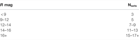
TABLE 1. Number of 1,000 frame sets as a function of target magnitude.
Previous papers (Horch et al., 2009, 2010; Howell et al., 2011) have discussed the relationships related to speckle decorrelation stating its linear dependence on the separation of two close point sources (stars) and its inverse dependence on the size of the isoplanatic patch. Taking ρ as the separation of two point sources (arssec), s as the seeing value (arcsec) and δs and the size of the isoplanatic patch (arcsec), we can define q′ (arcsec2) as follows: q′ = ρ/δs = ρs where s is inversely related to δs. Horch et al. (2010) and Scott et al. (2021) show that speckle decorrelation sets in when the seeing increases above ∼1.2” and/or q′ approaches ∼0.6 arcsec2, being certainly of concern when q′ is
2.2 Signal-to-Noise Calculations
As a proxy for the resulting S/N in a specific speckle final reconstructed image, we use the standard CCD equation modified to represent the particular image parameters and data collection procedures specific to speckle observations. In addition, the companion detection depends on the ability to robustly determine the background level and detect interferometric fringes in the processed short-exposure images. We will use known theoretical relationships (Dainty and Greenaway, 1979) for interferometric S/N determinations to provide modifications to the usual S/N equation, allowing us to calculate S/N estimates for speckle observations at Gemini. We will examine a few typical cases, that of bright (near full moon) and grey (full to quarter moon) sky and seeing values of 1.0 and 0.5″. The ranges considered herein provide a useful guide to allow an observer to estimate the desired result, such as the contrast limit, for a given observation.
We start by using Gemini’s listed values for their optical CCD imager, GMOS, as described in the GMOS integration time calculator3(ITC). We use the Gemini Observatory definitions for sky brightness and seeing4—that is image quality (IQ) yielding 0.5″ seeing is called 20%–Best and 1.0″ seeing is called 85–Poor. For the sky background brightness, we adopt 80%–Grey for times of quarter to near full moon or times of night before/after moon rise/set and Any/Bright for times of near full moon. We use the GMOS ITC values of the point spread function (PSF) spatial size at the focal plane for each seeing value considered and the sky background photons received per unit area for our modeled sky conditions. We assume an airmass of
The CCD S/N equation for a point source is given in §4.4 of Howell (2006) as
where N* is the total number of photons gathered from the source, npix is the number of pixels used for this S/N calculation, NS is the number of photons per pixel from the background or sky, ND is the number of dark current electrons per pixel, and NR is the number of electrons per pixel resulting from read noise. Zorro and ‘Alopeke use EMCCD imagers as described in Scott et al. (2021). For speckle imaging with an EMCCD, we can set the read noise
Thus, our S/N equation can be reduced to
which illustrates why the sky background level is a critical element here given the large number of pixels which the observed stellar PSF illuminates. For example, a PSF of 0.5″ FWHM covers 4,352 pixels in our images (which have plate scale of 0.01”/pixel), and at 1.0″ FWHM, 19,200 pixels are in the PSF. Thus, npix × NS can become substantial.
As a start, we take our CCD S/N calculation as above and check it against the GMOS ITC. Using GMOS values (e.g., pixel scale, filter) our calculations obtain answers that match those of the Gemini GMOS ITC to within 2%. Thus, we conclude that our implementation of Gemini telescope and GMOS observational parameters is accurate.
A stellar PSF at our speckle imaging plate scale covers a large area, and with a 0.06 s integration, the “PSF” is not a uniform Gaussian 2-D shape, but a set of many hundred randomly placed speckles, each containing few photons (e.g., Labeyrie, 1970; Scott et al., 2018, show illustrative speckle images). As the angular resolution achievable by an optical system becomes better, more photons are concentrated into each speckle, providing an increase in the S/N per frame. For our observations reported herein, this increase occurs with the better seeing and the larger collecting area of the Gemini 8-m telescope.
This complex speckle pattern S/N situation has been examined for some limiting cases by Welsh (1995), Petrov et al. (1986), and Dainty & Greenaway (1979). Following the discussions presented in these works, especially the latter, we modify the standard S/N equation such that N* is now the average number of detected photons per speckle (ns), where the number of speckles per frame is approximately given by
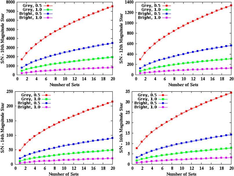
FIGURE 1. S/N for targets with R-band magnitudes of 10, 12, 14, and 16 as a function of the number of 1,000 frames sets. The curves are color-coded by sky condition (Grey, Bright) and seeing value (0.5″, 1.0″) as shown in the legend.
We can see that for bright stars (10th to 12th magnitude), the S/N is acceptable to very good for all cases under consideration. At 14th magnitude, poor seeing (∼ 1″) severely limits the resulting S/N in all cases considered herein. The bright sky during full moon can be compensated for by observing 10 or more 1000 frame sets especially under conditions of good seeing. At 16th magnitude, we see that only for very good seeing and grey skies is it possible to achieve decent S/N results, and then only by using 15–20 or more sets. Fainter targets have been successfully observed under good seeing conditions (0.4–0.6″) and dark to grey skies (Howell et al., 2016; 2021b). The S/N values calculated here will become less accurate as the target magnitude becomes fainter than 14th, since we used the “bright star” approximation in our S/N calculations as mentioned above and described in Dainty & Greenaway (1979).
As mentioned above, each short exposure represents an instantaneous view of the atmospheric distortions of the star’s wavefront frozen in time. From these images, the Fourier summation of the images into a power spectrum yields a diffraction limited view of the scene near the star, revealing other light sources (companions) within that field of view. Given the large areal coverage of the instantaneous PSF, we can use the S/N result above, noting that the S/N is proportional to 1/seeing2, to predict that a change in seeing of ±0.55″ will yield a change in the final achieved contrast level of about ±1.2 magnitudes at an angular separation of 0.5″ and ±2.5 magnitudes at 1.0″ (see Figure 1 and §3). Since any fringes produced by a multiple source will be of higher contrast as the flux ratio of the two (or more) sources approaches unity, nearly equal brightness binaries have an advantage over a pair of stars that have a delta magnitude value of, say, 6. Additionally, the S/N for a target, all else being equal, increases as the square root of the total integration time (i.e., number of sets) (e.g., Howell, 2006).
While we have used SDSS r filter parameters (which is centered at 630 nm), scaled to our 40 nm wide speckle filters, we would predict (and will see below) that better results will always be obtained at 832 nm, as the wavelength dependence of the Fried parameter r0 makes it about 1.8 times larger in the 832 nm sky. This larger “seeing cell” (isoplanatic patch) in turn directly correlates to the number of speckles in each image at each wavelength, being again about 1.8 times less at 832 nm than 562 nm, thus giving a higher S/N per speckle in the redder images. As is well known observationally (e.g., Kellerer and Tokovinin, 2007), better sky behavior in the red translates into the fact that the S/N is about 1.5–2 times better at 832 nm than at 562 nm, all else being equal. While we did not solve the equations for each specific wavelength, we will see below that the observational results at 832 nm are better in all aspects than those at 562 nm, and that our calculated change of ∼2 magnitudes of contrast for each 0.5″ seeing change matches the observations.
3 Results From Three Years of Speckle Observations
To compare the theoretical S/N calculations above with actual observations, we compiled the speckle data from all ‘Alopeke and Zorro runs from the 2019A, 2019B, 2020A, 2020B, 2021A, and 2021B semesters. For a uniform analysis, we only used data sets taken with the 562 and 832 nm filters, which constitute 90–95% of all observations. This amounted to a total of 935 and 1179 ′Alopeke data sets at 562 and 832 nm, respectively, and a total of 1138 and 1454 Zorro data sets at 562 and 832 nm, respectively (data sets where the target object was not detected were excluded; this mostly occurred for relatively faint targets at 562 nm which were observed for too short of a total time to robustly detect the faint star against the bright sky background). We used the resulting 5-σ contrast sensitivity curves from each observation, of which Figure 2 shows a representative example, to create plots that correlate the achieved sensitivity limits (contrast) at spatial distances of 0.2, 0.5 and 1.0″ with the seeing at the time of observations, the target’s airmass, and its V-band magnitude (Figures 3–6, 8, 9). We note here that we have switched to using V-band magnitudes in the following plots as these values are required from each PI for our observing lists and could be easily obtained. The majority of our observations presented in the following figures were obtained during bright sky conditions, often near full moon ±4 days.
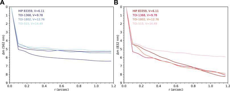
FIGURE 2. Representative speckle image contrast curves for a selection of stars observed with the Gemini North telescope using ‘Alopeke during semester 2020A. The curves show the 5σ contrast levels we reached in each case at 562 nm (A) and 832 nm (B) as a function of projected distance from the star. Note that the V = 9.8 target was observed in good seeing conditions (0.7″) at an airmass of 1.1 while the V = 6.1 target was observed at an airmass of 1.7 in poor seeing conditions (1.2″). Contrast curves such as these are produced for every observation, and the values used in Figures 3–9 give the measured contrast level at angular distances of 0.2, 0.5, and 1.0″ for each star.
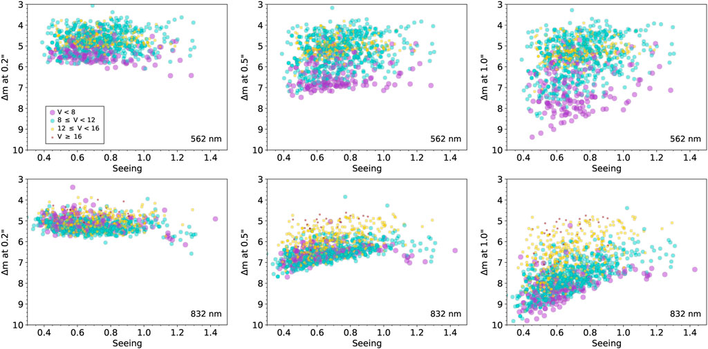
FIGURE 3. Results from ‘Alopeke observations in terms of how seeing (given in arcseconds) effects the contrast level achieved for a given target magnitude. The left panels show the limiting contrast values at 0.2″ from the target star, the middle panel the contrast at 0.5″, and the right panel the contrast at 1.0″. The top and bottom rows show the results for 562 nm data and 832 nm observations, respectively. The bins of target magnitude are color-coded and vary with symbol size as shown in the legend.
In Figures 3, 4, which show the contrast as a function of seeing for ’Alopeke and Zorro data, respectively, we can see that at 0.2″ the seeing has little effect on the limiting contrast, while at increasingly larger distances away from the target star, fainter targets do not allow the same contrast levels to be reached, especially at 562 nm. We note that in the 0.2″ plots in particular, it appears that we obtain greater contrasts for some bright stars when the seeing is poor (
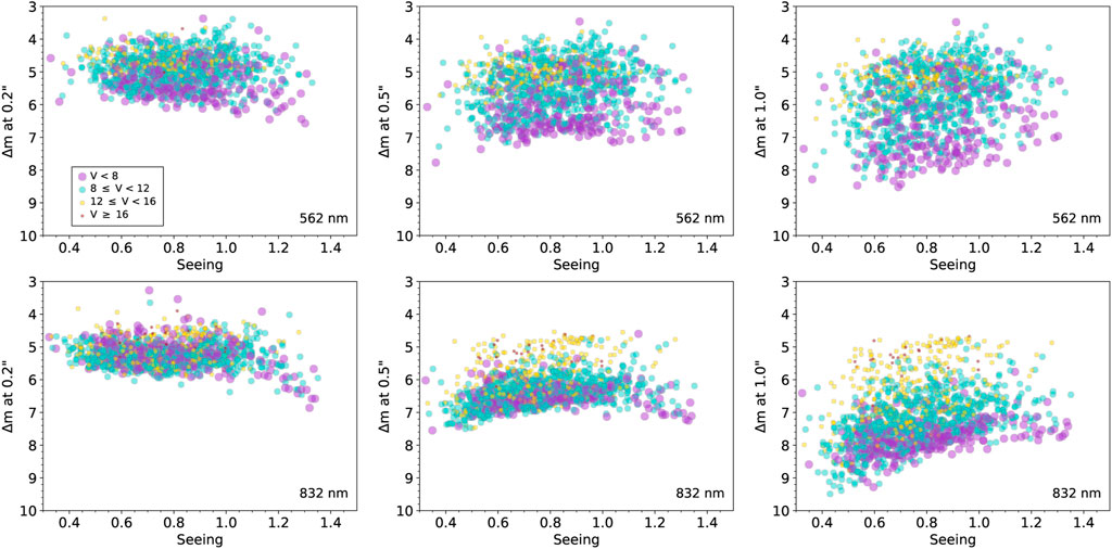
FIGURE 4. Similar to Figure 3, but showing the results from Zorro observations.
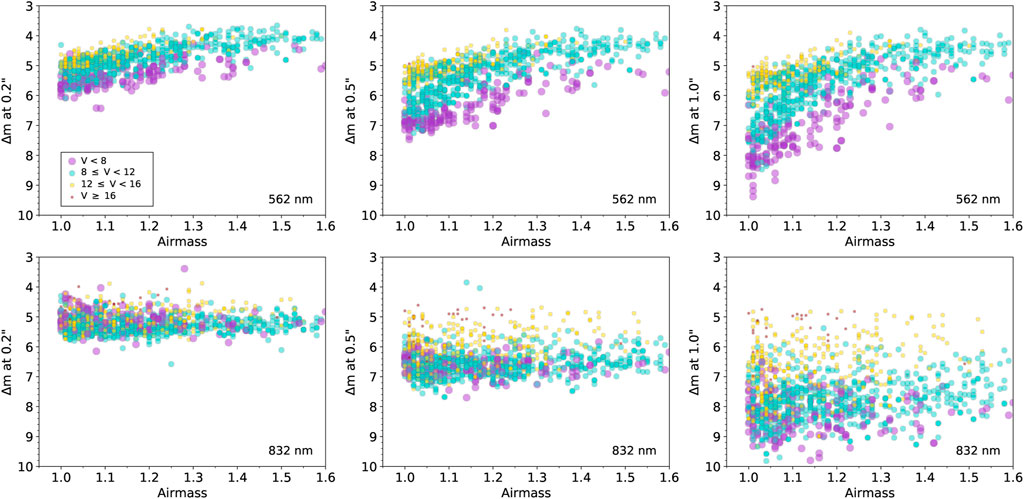
FIGURE 5. Similar to Figure 3, but showing the results in terms of how airmass effects the limiting contrast achieved for a given target magnitude.
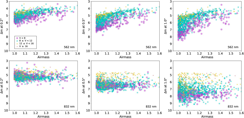
FIGURE 6. Similar to Figure 5, but showing the results from Zorro observations.
Overall, we see that 832 nm observations provide higher contrast levels for a given observation and are less effected by seeing and airmass. This is to be expected due to the far better atmospheric conditions at longer wavelength as well as the large decrease in background sky light under bright moon conditions compared to shorter wavelengths. We do note that in Figures 3–6, in general, Zorro observations at farther spatial distances (1.0″) show scatter across magnitude bins with bright and faint sources somewhat mixed together especially for 562 nm data. This is likely due to the lower elevation of the observatory and the typically fewer hours of very good seeing at Gemini South compared to Gemini North. As the seeing degrades, larger spatial distances from the target star can begin to exhibit speckle decorrelation (Howell et al., 2019), resulting in lower S/N.
We noted above (Figure 1) that our calculations allow us to relate the various seeing and sky conditions and the target brightness to the obtained S/N of the observation. In Figure 7 we show how the S/N values can be used to estimate the final contrast levels that are obtainable. Here we present an example for bright (R ∼10) and faint (R ∼14) targets showing the achieved contrast level under the range of seeing (0.5–1.0″) and sky conditions (grey and bright). For a faint source, the S/N values can be seen to degrade from 83 to 7.85 under the usual observational protocol of obtaining three sets of data and from grey skies with 0.5″ seeing to bright skies with 1.0″ seeing (see Figure 1, bottom left panel). The ratio 83/7.85 is a factor of about 10.6 or a difference of about 2.6 magnitudes. For a bright source, the S/N values range from 2924 to 314 (for three sets; see Figure 1, top left panel), giving a ratio of about 9.3 or 2.4 magnitudes. In each case, an increase in seeing of 0.5″ and an increase in sky brightness results in a drop in the contrast limit by about 2-3 magnitudes (see Figure 7). This observational result is in accordance with the predictions of S/N made in §2. Using the methodology shown in Figure 7, a robust estimation of the S/N and the contrast limits (Δm) for an observation can be made based on the total integration time used, the target brightness, and the seeing and sky conditions.
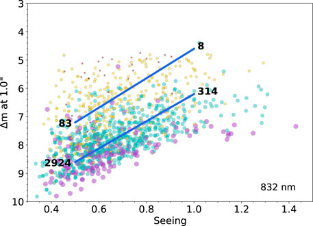
FIGURE 7. An example use of the S/N values shown in Figure 1, in which we reproduce the lower right panel of Figure 3 and overplot trend lines for a faint target (R ∼14, upper line) and a bright target (R ∼ 10, lower line). The numbers listed on the plot, taken from Figure 1, show the S/N values for a bright (R = 10) and a faint (R = 14) target at seeing values of 0.5 and 1.0″. Note the tendency to lose ∼2.5 magnitudes of limiting contrast when the seeing doubles. The symbols and color coding are the same as in Figure 3. See text for details.
Figures 8, 9 show the contrast as a function of target brightness for ’Alopeke and Zorro data, respectively. At 832 nm, the contrast limit at 0.2″ from the target star is relatively independent of target brightness (but requires more sets of observations for fainter targets), while it decreases at 0.5 and 1.0″ for fainter targets (V ≳ 15), despite the larger number of sets of observations. As noted in §2, to achieve equal contrasts for such faint targets, 50 or more sets (50 + minutes of total integration time) would be required (especially if observing conditions are not ideal), but to balance the amount of time spent on observations of each target, typically just ∼ 18–20 sets are taken of faint targets. Remarkably, for bright targets (V ≲ 8), just a few sets yield contrasts of ∼ 7 mag at a separation of 0.5″ and 7–10 mag at 1.0″. The results from Gemini North and South are similar overall, an interesting result given the very different altitudes of the two observatories.
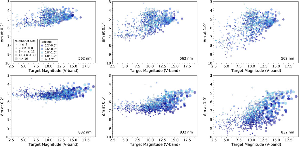
FIGURE 8. Combined results from the contrast curves of all ‘Alopeke observations from the 2019A to the 2021B semester showing Δ m values at spatial distances of 0.2, 0.5, and 1.0″ vs. the V-band magnitude of the target stars. The symbol size scales with the number of sets (where 1 set consists of 1,000 × 60 msec exposures), and the color scales with seeing (darker blue indicates better seeing conditions).
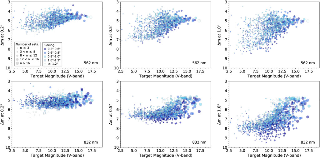
FIGURE 9. Similar to Figure 8, but for the Zorro observations from the 2019A to the 2021B semester.
4 Conclusion
The two speckle cameras ’Alopeke and Zorro on the Gemini North and South telescopes, respectively, offer high-resolution imaging in the optical wavelength range. We have shown that, depending on sky conditions (seeing, airmass) and target brightness, S/N ratios up to several 1000 can be achieved, which corresponds to contrast ratios of 4-5 magnitudes (close to the star, near the diffraction limit) up to 7–10 magnitudes at angular separations near 1.0″. The total time on target (observed as sets of 1000 × 60 ms frames) has to be increased, sometimes considerably, to achieve the desired S/N or limiting magnitude contrast level. We note that there are limitations due to the sky conditions, especially if the seeing deteriorates or the sky is highly illuminated by the moon. Satisfactory limiting contrast ratios and high-resolution, close companion detection have been achieved for targets as faint as R ∼19–20 by using 45–60 min of total integration time, i.e., many tens of 1000 frame sets. The two speckle instruments mounted on the twin 8-m Gemini telescopes are producing exciting science, from resolving very close (≤0.1″) binary companions, validating and confirming TESS exoplanets, imaging small bodies in the Solar System, to observational time domain astrophysics (see Scott et al., 2021). They are available for public use via the Gemini Observatory proposal process.
Data Availability Statement
The datasets presented in this study can be found in online repositories. The names of the repository/repositories and accession number(s) can be found in the article/Supplementary Material.
Author Contributions
All authors listed have made a substantial, direct and intellectual contribution to the work, and approved it for publication.
Funding
All funding was provided by NASA research grants.
Conflict of Interest
The authors declare that the discussion and research was conducted in the absence of any commercial or financial relationships that could be construed as a potential conflict of interest.
Publisher’s Note
All claims expressed in this article are solely those of the authors and do not necessarily represent those of their affiliated organizations, or those of the publisher, the editors and the reviewers. Any product that may be evaluated in this article, or claim that may be made by its manufacturer, is not guaranteed or endorsed by the publisher.
Acknowledgments
The authors wish to recognize and acknowledge the very significant cultural role and reverence that the summit of Maunakea has always had within the indigenous Hawaiian community. We are most fortunate to have the opportunity to conduct observations from this mountain. We wish to thank the many staff members at the Gemini Observatory who have helped us with this observational program over the years. In particular, Andrew Stephens, Ricardo Salinas, Alison Peck, John White, and Andy Adamson. We also wish to thank the dedicated members of our speckle team that made the entire program happen: Elliott Horch, Mark Everett, Nic Scott, David Ciardi, Rachel Matson, Crystal Gnilka, and Katie Lester. This paper made use of observational data obtained with the High-Resolution Imaging instruments ‘Alopeke and Zorro, mounted on the Gemini North and Gemini South telescopes respectively. The authors thank Andy Adamson for his comments on a draft manuscript. All of the data is public and available at the NASA Exoplanet Archive. ‘Alopeke and Zorro were funded by the NASA Exoplanet Exploration Program and built at the NASA Ames Research Center by SH, Nic Scott, Elliott P. Horch, and Emmett Quigley. The International Gemini Observatory, a program of NSF’s OIR Lab, is managed by the Association of Universities for Research in Astronomy (AURA) under a cooperative agreement with the National Science Foundation. on behalf of the Gemini partnership: the National Science Foundation (United States), National Research Council (Canada), Agencia Nacional de Investigación y Desarrollo (Chile), Ministerio de Ciencia, Tecnología e Innovación (Argentina), Ministério da Ciência, Tecnologia, Inovações e Comunicações (Brazil), and Korea Astronomy and Space Science Institute (Republic of Korea). Facilities: Gemini–‘Alopeke, Zorro.
Footnotes
1https://en.wikipedia.org/wiki/Speckle_imaging.
2https://exofop.ipac.caltech.edu/tess/.
3https://www.gemini.edu/instrumentation/gmos/exposure-time-estimation.
4https://www.gemini.edu/observing/resources/itc/itc-help.
References
Chontos, A., Huber, D., Berger, T. A., Kjeldsen, H., Serenelli, A. M., Silva Aguirre, V., et al. (2021). TESS Asteroseismology of α Mensae: Benchmark Ages for a G7 Dwarf and its M Dwarf Companion. Astronomical J. 922, 229. doi:10.3847/1538-4357/ac1269
Dainty, J. C., and Greenaway, A. H. (1979). in IAU Colloq. 50: High Angular Resolution Stellar Interferometry. Editors J. Davis, and W. J. Tango, 23–1–23–17.
Fried, D. L. (1966). Optical Resolution through a Randomly Inhomogeneous Medium for Very Long and Very Short Exposures. J. Opt. Soc. Am. 56, 1372. doi:10.1364/josa.56.001372
Horch, E. P., Falta, D., Anderson, L. M., DeSousa, M. D., Miniter, C. M., Ahmed, T., et al. (2010). Ccd Speckle Observations of Binary Stars with the Wiyn Telescope. Vi. Measures during 2007-2008. Astronomical J. 139, 205–215. doi:10.1088/0004-6256/139/1/205
Horch, E. P., Gomez, S. C., Sherry, W. H., Howell, S. B., Ciardi, D. R., Anderson, L. M., et al. (2011). Observations of Binary Stars with the Differential Speckle Survey Instrument. II. Hipparcos Stars Observed in 2010 January and June. Astronomical J. 141, 45. doi:10.1088/0004-6256/141/2/45
Horch, E. P., Howell, S. B., Everett, M. E., and Ciardi, D. R. (2012). Observations of Binary Stars with the Differential Speckle Survey Instrument. IV. Observations of Kepler, CoRoT, and Hipparcos Stars from the Gemini North Telescope. Astronomical J. 144, 165. doi:10.1088/0004-6256/144/6/165
Horch, E. P., Veillette, D. R., Baena Gallé, R., Shah, S. C., O'Rielly, G. V., and van Altena, W. F. (2009). Observations of Binary Stars with the Differential Speckle Survey Instrument. I. Instrument Description and First Results. Astronomical J. 137, 5057–5067. doi:10.1088/0004-6256/137/6/5057
Howell, S. B., Everett, M. E., Horch, E. P., Winters, J. G., Hirsch, L., Nusdeo, D., et al. (2016). Speckle Imaging Excludes Low-Mass Companions Orbiting the Exoplanet Host Star Trappist-1. Astronomical J. 829, L2. doi:10.3847/2041-8205/829/1/L2
Howell, S. B., Everett, M. E., Sherry, W., Horch, E., and Ciardi, D. R. (2011). Speckle Camera Observations for the NASA Kepler Mission Follow-Up Program. Astronomical J. 142, 19. doi:10.1088/0004-6256/142/1/19
Howell, S. B., Scott, N. J., Matson, R. A., Everett, M. E., Furlan, E., Gnilka, C. L., et al. (2021a). The NASA High-Resolution Speckle Interferometric Imaging Program: Validation and Characterization of Exoplanets and Their Stellar Hosts. Front. Astron. Space Sci. 8, 10. doi:10.3389/fspas.2021.635864
Howell, S. B., Scott, N. J., Matson, R. A., Horch, E. P., and Stephens, A. (2019). High-resolution Imaging Transit Photometry of Kepler-13AB. Astronomical J. 158, 113. doi:10.3847/1538-3881/ab2f7b
Howell, S. B., Shen, Y., Furlan, E., Gnilka, C. L., and Stephens, A. W. (2021b). Gemini Speckle Imaging of Dual Quasar Candidates. Res. Notes AAS 5, 210. doi:10.3847/2515-5172/ac26c8
Kellerer, A., and Tokovinin, A. (2007). Atmospheric Coherence Times in Interferometry: Definition and Measurement. Astronomy Astrophysics 461, 775–781. doi:10.1051/0004-6361:20065788
Petrov, R., Roddier, F., and Aime, C. (1986). Signal-to-noise Ratio in Differential Speckle Interferometry. J. Opt. Soc. Am. A 3, 634. doi:10.1364/JOSAA.3.000634
Scott, N. J., Howell, S. B., Gnilka, C. L., Stephens, A. W., Salinas, R., Matson, R. A., et al. (2021). Twin High-Resolution, High-Speed Imagers for the Gemini Telescopes: Instrument Description and Science Verification Results. Front. Astron. Space Sci. 8, 138. doi:10.3389/fspas.2021.716560
Scott, N. J., Howell, S. B., Horch, E. P., and Everett, M. E. (2018). The NN-Explore Exoplanet Stellar Speckle Imager: Instrument Description and Preliminary Results. PASP 130, 054502. doi:10.1088/1538-3873/aab484
Keywords: instrumentation–telescopes, speckle imaging, Gemini telescope, techniques, high resolution imaging
Citation: Howell SB and Furlan E (2022) Speckle Interferometric Observations With the Gemini 8-m Telescopes: Signal-to-Noise Calculations and Observational Results. Front. Astron. Space Sci. 9:871163. doi: 10.3389/fspas.2022.871163
Received: 07 February 2022; Accepted: 25 April 2022;
Published: 01 June 2022.
Edited by:
Maud Langlois, UMR5574 Centre de recherche astrophysique de Lyon (CRAL), FranceReviewed by:
David Leisawitz, National Aeronautics and Space Administration, United StatesVincent Deo, National Astronomical Observatory of Japan (NINS), Japan
Copyright © 2022 Howell and Furlan. This is an open-access article distributed under the terms of the Creative Commons Attribution License (CC BY). The use, distribution or reproduction in other forums is permitted, provided the original author(s) and the copyright owner(s) are credited and that the original publication in this journal is cited, in accordance with accepted academic practice. No use, distribution or reproduction is permitted which does not comply with these terms.
*Correspondence: Steve B. Howell, c3RldmUuYi5ob3dlbGxAbmFzYS5nb3Y=
†ORCID: Steve B. Howell, orcid.org/0000-0002-2532-2853; Elise Furlan, orcid.org/0000-0001-9800-6248