
95% of researchers rate our articles as excellent or good
Learn more about the work of our research integrity team to safeguard the quality of each article we publish.
Find out more
REVIEW article
Front. Astron. Space Sci. , 06 January 2023
Sec. Stellar and Solar Physics
Volume 9 - 2022 | https://doi.org/10.3389/fspas.2022.1060862
This article is part of the Research Topic Flare Observations in the IRIS Era: What Have We Learned, and What’s Next? View all 10 articles
 Graham S. Kerr1,2*
During solar flares a tremendous amount of magnetic energy is released and transported through the Sun’s atmosphere and out into the heliosphere. Despite over a century of study, many unresolved questions surrounding solar flares are still present. Among those are how does the solar plasma respond to flare energy deposition, and what are the important physical processes that transport that energy from the release site in the corona through the transition region and chromosphere? Attacking these questions requires the concert of advanced numerical simulations and high spatial-, temporal-, and spectral-resolution observations. While flares are 3D phenomenon, simulating the NLTE flaring chromosphere in 3D and performing parameter studies of 3D models is largely outwith our current computational capabilities. We instead rely on state-of-the-art 1D field-aligned simulations to study the physical processes that govern flares. Over the last decade, data from the Interface Region Imaging Spectrograph (IRIS) have provided the crucial observations with which we can critically interrogate the predictions of those flare loop models. Here in Paper 2 of a two-part review of IRIS and flare loop models, I discuss how forward modelling flares can help us understand the observations from IRIS, and how IRIS can reveal where our models do well and where we are likely missing important processes, focussing in particular on the plasma properties, energy transport mechanisms, and future directions of flare modelling.
Solar flares are transient, broadband brightenings to the Sun’s radiative output following the liberation of a tremendous amount of energy (up to 1032 erg, or larger: Emslie et al., 2012; Aschwanden et al., 2015) during magnetic reconnection (e.g., Priest and Forbes, 2002; Shibata and Magara, 2011; Janvier et al., 2013; Emslie et al., 2012). It is thought that this energy is subsequently transported predominately in the form of non-thermal particles. We primarily consider non-thermal electrons1, accelerated during the reconnection process. Once they reach the denser lower solar atmosphere they thermalise via Coulomb collisions (e.g., Brown, 1971), heating and ionising the plasma and generating mass flows: chromospheric evaporation (upflowing material) and chromospheric condensations (downflowing material). Alternative mechanisms of energy transport in flares include non-thermal protons or heavier ions, thermal conduction following direct heating of the corona, and Alfvénic waves, discussed in more detail in Section 3.
There is unambiguous evidence for the presence of non-thermal particles in flares, due to the hard X-rays they produce via bremsstrahlung. Their ubiquitousness and the close spatial and temporal association with other flare emission (e.g., optical and UV) has bolstered the ‘electron-beam’ model of solar flares. Observations of hard X-rays, e.g., from the Reuven Ramaty High Energy Solar Spectroscopic Imager (RHESSI; Lin et al., 2002), can be used to infer the underlying non-thermal electron energy distribution, that itself can drive models of solar flares. There is a substantial body of literature describing the various characteristics of flares, and the means in which we observe them. I direct the reader towards the following reviews of flare observations, and flare particle acceleration and thermalisation: Benz (2008); Fletcher et al., 2011; Holman et al., 2011; Kontar et al., 2011; Zharkova et al., 2011; Milligan (2015). The bulk of the flare radiative output originates from the chromosphere and transition region, making those regions important areas of study for their diagnostic potential regarding the plasma response to energy injection, and the energy transport and release process themselves. However, speaking candidly, this potential has been somewhat squandered by the lack of routine high spatial-, temporal-, and spectral-observations of the chromosphere and transition region at UV wavelengths during flares (crucially, we lacked routine imaging spectroscopy of the flare chromosphere). That observational gap has fortunately been plugged following the launch of the Interface Region Imaging Spectrograph (IRIS; De Pontieu et al., 2014); in 2013, that now gives us an unprecedented view of the flaring chromosphere and transition region, yielding crucial new insights. Given the complex environment of these particular layers, parallel efforts to forward model the flaring lower atmosphere, and its impacts on the flaring corona, are required to make substantial progress in understanding the physics at play in flares.
This is the second paper in a two part review of how solar flare loop models in concert with IRIS observations have improved our understanding of solar flares. Between both parts I hope to emphasise that it is only by attacking the problem of flare physics via the combination of high quality observations and state-of-the-art models, that include the pertinent physical processes, that we can make rapid progress. Overall I aim to show: 1) how modelling has helped interpret the IRIS observations; 2) how IRIS observations have been used to interrogate and validate model predictions; and 3) how, when models fail to stand up to the stubborn reality of those observations, IRIS has led to model improvements. In Paper 1 of this review (Kerr, 2022) I provided a detailed overview of each numerical code, and discussed what we have learned from the study of Doppler motions from IRIS in the context of the non-thermal electron beam driven flare model. Also in Paper one is a more extensive introduction to solar flares. Here in Paper 2 I demonstrate how we have used the combination of IRIS and flare loop modelling to learn about plasma properties and flare energy transport mechanisms, and provide some thoughts on future directions.
IRIS is a NASA Small Explorer mission that has observed many hundreds of flares, including dozens of M and X class events. Both images (via the slit-jaw imager, SJI) and spectra (via the slit-scanning spectrograph, SG) are provided in the far- and near-UV (FUV and NUV), with a spatial resolution 0.33–0.4 arcseconds. High cadences are achievable, as low as 1 s but more generally a few seconds to tens of seconds. The strongest lines observed are Mg ii h 2,803 Å and k 2,796 Å lines (chromosphere), C ii 1,334 Å and 1,335 Å and Si iv 1,394 Å and 1,403 Å (transition region), and Fe xxi 1,354.1 Å (
The models employed to study flares are generally field-aligned (1D) numerical codes (though there are some exceptions, e.g., the 3D radiative magnetohydrodynamic, MHD, model of Cheung et al., 2019). These codes are nimble enough to be run on timescales that make performing parameter studies of flare energy transport processes a tractable activity, and they allow us to include the relevant physical processes at the required spatial resolution (down to sub-metres) that is not yet feasible in 3D RMHD simulations. I focus on the RADYN, HYDRAD, FLARIX, and PREFT models here. A brief overview is presented below but see Paper 1 for a full description of each code.
The hydrodynamic field-aligned codes HYDRAD (Bradshaw and Mason, 2003a; Bradshaw and Mason, 2003b; Reep et al., 2013; Reep et al., 2019), RADYN (Carlsson and Stein, 1992; Carlsson and Stein, 1997; Carlsson and Stein, 2002; Abbett and Hawley, 1999; Allred et al., 2005; Allred et al., 2015), and FLARIX (Kas̆parová et al., 2009; Varady et al., 2010; Heinzel et al., 2016) are now well established and widely used by the solar flare community. These codes solve the equations describing the conservation of mass, momentum, charge, and energy in a single field-aligned magnetic strand rooted in the photosphere and stretching out to include the chromosphere, transition region, and corona. HYDRAD and RADYN use an adaptive grid where the size of the grid cells can vary to allow shocks and steep gradients in the atmosphere to be resolved as required (with HYDRAD varying the number of grid cells also), while FLARIX uses a fixed, but optimized, grid with
All three simulate the response of the atmosphere to injection of energy, typically via a beam of non-thermal electrons (but flare-accelerated ions can be included too). RADYN uses a Fokker-Plank treatment to model the evolution of the non-thermal electron distribution as a function of time (including return current effects), that was recently updated to use the standalone state-of-the-art non-thermal particle transport code FP2 (Allred et al., 2020). HYDRAD uses the analytic treatment of Emslie (1978) and Hawley and Fisher (1994), and FLARIX uses a test-particle module that provides the time-dependent beam propagation including scattering terms. Dissipation of Alfvénic waves has also been implemented in both HYDRAD and RADYN (Reep and Russell, 2016; Reep et al., 2018b; Kerr et al., 2016), and all codes can include ad hoc time dependent heating.
Each code has been conceived and developed to focus on particular details of the flaring plasma physics problem. RADYN and FLARIX are radiation hydrodynamic codes which couple the hydrodynamic equations to the non-LTE (NLTE) 1D radiative transfer and time-dependent non-equilibrium atomic level population equations, for elements important for chromospheric energy balance. RADYN considers H, He and Ca, with Mg also sometimes included, whereas FLARIX considers H, Ca, and Mg (with plans to update the code to include He). Continua from other species are treated in LTE as background metal opacities. Optically thin losses are included by summing all transitions from the CHIANTI atomic database (Dere et al., 1997; Del Zanna et al., 2015; Del Zanna et al., 2021)3 apart from those transitions solved in detail. Additional backwarming and photoionisations by soft X-ray, extreme ultraviolet, and ultraviolet radiation is included. Both currently use the assumption of complete frequency redistribution (CRD)4 when solving the radiation transport problem, so that post-processing via other radiation transport codes such as RH (Uitenbroek, 2001), RH15D (Pereira and Uitenbroek, 2015), or MALI (Heinzel, 1995) is required. In RADYN and FLARIX the loop is modelled as one leg of a symmetric flux tube. RADYN also allows to calculate aposteriori (i.e. with no feedback on the plasma equations of mass, momentum, and energy) the time-dependent non-equilibrium populations and radiation transport of a desired ion via the minority species version of that code, MS_RADYN (Judge et al., 2003; Kerr et al., 2019b; Kerr et al., 2019c).
HYDRAD does not solve the detailed optically thick radiation transport and atomic level population equations, instead employing approximations of chromospheric radiation losses. Losses from H, Ca and Mg are included via the approach of Carlsson and Leenaarts (2012). The code has also recently adopted a more accurate method for computing NLTE H populations following the prescription of Sollum (1999) which approximates the radiation field in the chromosphere (Reep et al., 2019). Ion population equations, however, are solved self-consistently in full non-equilibrium ionization (NEI) for any desired element, returning a more accurate calculation of the optically thin radiative losses and spectral synthesis of optically thin lines using those ion fractions. While the treatment of optically thick radiation is less robust than in RADYN or FLARIX, HYDRAD has the advantage of being significantly less computationally demanding. Other important differences are that HYDRAD features a multi-fluid plasma that treats the electron and hydrogen temperatures separately, it solves a full length flux tube (foot-point to foot-point) of arbitrary geometry (e.g., based on a magnetic field extrapolation) and includes effects due to cross-sectional area expansion (varying inversely with the magnetic field strength), which has been shown to play an important role in dynamics (Reep et al., 2022).
PREFT (Guidoni and Longcope, 2010; Longcope and Guidoni, 2011; Longcope and Klimchuk, 2015; Longcope et al., 2016) is a rather different code than the other three, and is a powerful tool to study the impact of magnetic loop dynamics during flares. It is a 1D MHD code that solves the thin flux tube (TFT) equations. The tube is initialized at the instant after a localized reconnection process within the current sheet has linked sections of equilibrium tubes from opposite sides of the current sheet. No further reconnection occurs, and any heating from the initializing event is neglected. In its subsequent evolution, the tube retracts under magnetic tension releasing magnetic energy and converting it to bulk kinetic energy in flows which include a component parallel to the tube. The collision between the parallel components generates a pair of propagating slow magnetosonic shocks, which resemble gas dynamic shocks as they must in the parallel limit. Radiative losses are optically thin, and normally an isothermal, but gravitationally stratified, chromosphere is included mostly as a mass reservoir. Solutions of the TFT equations show that thermal conduction carries heat away from the shocks, drastically altering the temperature and density of the post-flare plasma (Longcope and Guidoni, 2011; Longcope and Klimchuk, 2015; Longcope et al., 2016; Unverferth and Longcope, 2020).
Since much of emission from the flaring chromosphere is optically thick, extracting meaningful information about the plasma properties is difficult and often requires forward modelling from flare simulations in order to interpret observations. Even in the corona where emission is optically thin, modelling is required. In this section I present some examples of where flare models have shed light on conditions in the flare atmosphere.
The flare chromosphere has been studied extensively using optically thick lines, which while presenting challenges with respect to extracting useful information due to their complex formation properties, offer important diagnostics of how the plasma responds to flares. Most notably, the Hα line has been both observed and modelled in flare studies too numerous to exhaustively list or describe in detail here. Some examples include: Canfield and Ricchiazzi (1980), Canfield et al., 1984, Canfield and Gayley (1987), Canfield et al. (1991), Heinzel (1991), Gayley and Canfield (1991), Gan et al., 1992, Gan et al., 1993, Li et al., 2006, Kuridze et al., 2015, Rubio da Costa et al. (2015). Some important numerical results inform us about how conditions in the upper chromosphere result in varying characteristics of the line, such as the depth of central reversal, are related to plasma conditions. The coronal pressure, for example, was found to be an important factor in determining the depth of the central reversal, with a high coronal pressure (
In this section I introduce the Mg ii NUV spectra as observed by IRIS, which being one of the strongest lines in the IRIS passbands has become a workhorse for studying the chromosphere, including during flares. Like the spectral lines of hydrogen and calcium, their characteristics are very sensitive to atmospheric properties, with various flare effects changing both the formation location as well as local plasma conditions. Magnesium is 18 times more abundant than Calcium, consequently forming higher in altitude and sampling the upper chromosphere, a useful region for understanding energy deposition during flares. The Mg ii h and k Doppler width is much smaller than that of Hα, offering advantages in sensitivity to both Doppler motions and turbulence.
The Mg ii NUV spectra, comprising the h and k resonance lines (λ2,803.52 Å and λ2,796.34 Å, respectively), the subordinate triplet (λ2,791.60 Å, λ2,798.75 Å and λ2,798.82 Å, the latter two of which are blended), and who’s lower energy levels are the upper levels of the resonance lines, and the quasi-continuum that lies between them, offer a wealth of information about the chromosphere. As some of the strongest and most commonly observed lines in the IRIS dataset, they have been well studied both observationally and in models. They are, however, somewhat of a menace to interpret, requiring complicated radiation transfer modelling including partial frequency redistribution (PRD; meaning there is a coherency between incident and scattered photons, which effects conversion of photons from core to wing) to help extract the information they carry. Obtaining a strong almost one-to-one match even in the quiet Sun still proves very challenging, likely due to both the complexity of the radiation transfer involved, and the assumed model atmospheres (the main chronic problem is the line width, which is much too narrow in simulations). While we make progress in obtaining more consistent model-data comparisons we learn more about the formation properties of the lines and the flaring conditions that we can infer about the plasma.
The Mg ii lines were comprehensively studied in the quiescent chromosphere most recently by Leenaarts et al. (2013a), Leenaarts et al. (2013b) and Pereira et al. (2013). While in active regions and flares their formation properties likely deviate from the description that follows, the quiescent studies form a basis for understanding these strong lines. These lines form throughout the chromosphere, with cores forming in the upper chromosphere, and wings forming from the upper photosphere through mid chromosphere. The resonance lines appear centrally reversed in most quiet Sun conditions (sunspots being the notable exception, though there the subordinate lines remain in absorption), with the core flanked by two emission peaks. The core is referred to as the k3 (or h3) component, and the emission peaks are collectively the k2 (or h2) components, with the blue peak referred to as k2v (or h2v) and the red peak as k2r (or h2r). Figure 1 shows both a quiet Sun and flare Mg ii k profile to illustrate these features. This central reversal forms because the line source function is decoupled from the Planck function (that is, the local temperature), and falls with increasing altitude, so intensity at the height at which optical depth is unity (τλ = 1; the surface from which we see the emergent intensity at some λ) is smaller than the intensity of the emission peaks, which have a slightly smaller opacity and form somewhat deeper. Their width, the asymmetry of the strength of the flanking peaks, their intensity, the depth of the reversal, and the k/h intensity ratio all show variations depending on the source conditions (e.g., Lemaire and Skumanich, 1973; Kohl and Parkinson, 1976; Lemaire et al., 1981). The k/h intensity ratio5, Rk:h, has a typical value around Rk:h = 1.2, indicative of optically thick line formation (Rk:h = 2, the ratio of their oscillator strengths, in optically thin formation conditions). The subordinate lines are generally in absorption, unless there is additional heating at large column depth where they typically form (e.g., Pereira et al., 2015). Note that modelling suggests that in the flaring case, the subordinate lines form much higher in altitude, and so subordinate line emission in flares is likely not a signature of deep heating, instead representing a heated mid-upper chromosphere (see, e.g., Kerr et al., 2019c; Zhu et al., 2019).
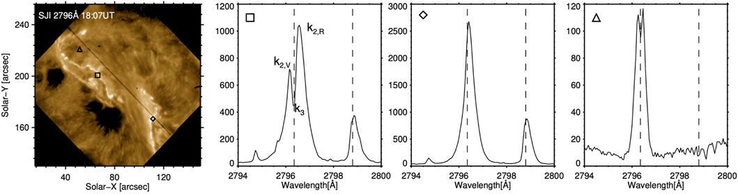
FIGURE 1. An illustration of the Mg ii profiles as observed by IRIS. The map on the left shows a flare image from the SJI. The spectra in the other three panels come from the locations identified by symbols on the map. The square (second panel) is a profile from the leading edge of a flare ribbon, where the different line components are labelled. The diamond (third panel) is a source in the middle of a flare ribbon. The triangle (fourth panel) is a profile from the quiet Sun. Figure adapted from Polito et al., 2022. Reproduced with permission.
In flares the Mg ii h and k profiles are seen to significantly increase their intensity (by several factors to greater than an order of magnitude), broaden (with FWHM > 1 Å, compared to FWHM < ∼ 0.5 Å pre-flare), exhibit redshifted cores (several tens of km s−1) and/or extreme red wing asymmetries, and to fill in their central reversal, appearing single peaked or with only a very shallow reversal (e.g., Kerr et al., 2015; Liu et al., 2015; Panos et al., 2018). These lines can appear rather Lorentzian in shape in many flare spectra. The subordinate lines come into emission and display many of the same characteristics as the resonance lines. In some cases, blue wing asymmetries are observed (e.g., Kerr et al., 2015; Tei et al., 2018; Huang et al., 2019). The k/h line intensity ratios during flares still indicate optically thick emission, and have been reported to decrease slightly. Kerr et al., 2015 found Rk:h = 1.07–1.19 in an M-class flare, and Panos et al., 2018 found an average of Rk:h = 1.16 from their larger survey. The range of observed Rk:h values seems smaller in the flaring region (Kerr et al., 2015). Finally, Xu et al. (2016) and Panos et al., 2018 found that profiles located at the leading edge of some flare ribbons appeared very different to the profiles located in the bright ribbon segments. They contained deep central reversals, were much broader, had slightly blueshifted cores, and asymmetric emission peaks. The Mg ii profiles from flares can vary on short timescales and small spatial scales (sometimes frame-to-frame, and pixel-by-pixel), suggesting they are extremely sensitive to plasma conditions, and therefore flare energy input.
Efforts to model the Mg ii spectra with electron beam driven flare simulations generally leads to profiles that behave qualitatively as we might expect, but contain important quantitative issues (e.g., Liu et al., 2015; Kerr, 2017; Kerr et al., 2016; Rubio da Costa et al., 2016; Kerr et al., 2019a; Kerr et al., 2019b). For example results from RADYN + RH or using semi-empirical flare atmospheres shows that the Mg ii spectra have an intensity increase (but are usually too intense, by up to approximately an order of magnitude or more), have redshifts and red-wing asymmetries (but the occasionally observed blue-wing asymmetries are harder to explain in the models), are broadened (but are significantly more narrow in the mid-far wings than observations, with observations in the range FWMH ∼ [0.5–2] Å but in typical modelling FWHM < 0.5 Å), have subordinate lines in emission (but which are also too narrow and too weak relative to the resonance lines, by up to several factors), and have shallower central reversals (but it is difficult to synthesise the single peaked spectra that are observed). Understanding the source of these differences can lead us to better understanding of plasma conditions and how to improve our modelling efforts to obtain those conditions.
In a data-driven study of the 2014-March-29th X-class flare Rubio da Costa et al. (2016) analysed Mg ii k line observations, comparing them to forward modelling using RADYN + RH. RHESSI hard X-ray observations were used to obtain the non-thermal electron distribution over time, using 2,796 Å IRIS SJI flare source areas to estimate the energy fluxes (which ranged F ∼ [4 × 10¹⁰–1011] erg s−1 cm−2), and were split into 16 ‘threads’, the timings of which were defined by the derivative of the GOES X-ray Sensor-B channel (XRS-B; 1-8Å soft X-rays). Each individual peak in the soft X-ray derivative was proposed to represent the injection of particles into the chromosphere, and the duration of the heating phase of each thread was taken from the duration of each soft X-ray peak. These threads were individually processed through RH to synthesise Mg ii spectra, and were subsequently averaged in time to mimic the contribution from multiple threads over the flaring area (the heating and relaxation times of some threads overlapped). IRIS spectra were averaged over the source region of hard X-rays, and compared to the thread-averaged synthetic spectra. As hinted above, this comparison was less than ideal, with synthetic Mg ii spectra having central reversals in the cores, that were much too narrow, and which at times exhibited blueshifts. There were some qualitative matches, however, with strong intensity enhancements and downflows producing redshifted line cores of up to a few tens of km s−1. Contrary to what is suggested by Rubio da Costa et al. (2016), I think that the presence of a strong k2v peak in the synthetic spectra is indicative of a strong downflow in the upper chromosphere in the model, rather than upflows. In their Figure 13, it can be seen that the line core (the centrally reversed part of the line) is redshifted, indicating a downflow. This would shift the absorption profile to the red, meaning that k2r photons from the red peak are more strongly absorbed than k2v blue peak photons that can more easily escape. The result is a brighter blue peak relative to red peak, producing an asymmetry. The effect of mass flows on the absorption of emission in optically thick lines has been discussion in detail in the context of Ca ii, Hα, and Mg ii in both acoustic shocks and flares: Carlsson and Stein (1992); Kuridze et al., 2015; Kerr et al., 2016.
To address the sources of these model-data discrepancies Rubio da Costa et al. (2016) studied the line formation properties and manually varied a snapshot of the RADYN atmosphere input to RH, introducing microturbulence. They found that introducing a large microturbulent velocity (vturb = 27 km s−1, compared to the vturb = 10 km s−1 assumed in the original model) could broaden the line core, but could not model the extended wings. A similar conclusion was reached by Huang et al., 2019, who performed a model-data study comparing a flare jointly observed by IRIS and Big Bear Solar Observatory/Goode Solar Telescope (BBSO/GST; Goode and Cao, 2012) to an F-CHROMA RADYN model database6 with inputs most closely aligned with non-thermal electron distribution parameters discerned from RHESSI hard X-rays. They processed snapshots of that simulation through RH15D, with different values of vturb = [10, 20, 30] km s−1, and while it seems that a single value of turbulent velocity was not able to appropriately model the line, a weighted combination was more successful at capturing the width at the time a blue-wing asymmetry appeared, which was the main focus of that work. A means to estimate the actual turbulent velocity in flares that contributes to line broadening is to measure the non-thermal line width of an optically thin line (or ideally multiple lines), which does not suffer from opacity broadening effects that muddy the waters. There are not many strong optically thin lines originating and often observed in the chromosphere so obtaining this value at multiple formation temperatures is difficult, but even a rough guide would be very useful. The O i 1,355.6 Å line observed by IRIS is optically thin in the quiet Sun (Lin and Carlsson, 2015), and preliminary modelling results suggests that it remains so during flares (e.g. Kerr et al., 2019c, plus Prof. M. Carlsson private communication 2022). This line has been relatively little studied observationally, but some estimates of vnthm ∼ 9–10 km s−1 were obtained in an M class flare (Kerr, 2017), and similar values have been seen in C-class flares (Dr. Sargam Mulay, private communication 2022), a slight increase from the
Returning to Rubio da Costa et al. (2016), they also experimented with manually raising the electron density by a factor of 10 (to ne > 1014 cm−3) in a narrow region at the base of the transition region (though not in a self-consistent manner so that the temperature and other properties were fixed), which had the effect of filling in the central reversal. This was because the larger density allowed a greater degree of collisional coupling to local conditions7, and the Mg ii k line core source function increased with height, tracking the rise of the Planck function more closely, past the point at which the τλ = 1. This suggests that in actual flares, extremely large densities are present in the upper chromosphere/lower transition region, to drive the line to appearing single peaked.
Given the discrepancies identified by Rubio da Costa et al. (2016) and other authors Rubio da Costa and Kleint (2017), decided to perform a much larger parametric study to determine what aspects of the flaring atmosphere had to change in order to produce Mg ii NUV spectra more consistent with observations. They took a snapshot from one of the RADYN simulations from Rubio da Costa et al. (2016), and manually varied the temperature, electron density, and velocity structure of the flaring chromosphere in a systematic way, that were processed through RH. They varied one parameter at a time, and did not re-solve the atmosphere to hydrostatic equilibrium given the updated parameter, in order to discern the direct impact of, for example, temperature variations by itself. This means that charge was not conserved in their models, and the atmospheres investigated were not self-consistent. Still Rubio da Costa and Kleint (2017), provided great insights into plasma conditions that could be producing the observed profiles.
Introducing a steeper temperature rise in the upper chromosphere through the transition region 8, the formation region of the Mg ii h and k line cores, led to weaker (by a factor
Enhancing the electron density by a factor of ten through the formation region of the resonance line cores9 produced single peaked profiles, and actually drove the k:subordinate line ratio closer to observations (Rk:sub ∼ 8, so within a factor two of the observations), though also increased the line intensity by around a factor of two. This is illustrated in the lefthand side of Figure 2, which shows the Mg ii NUV spectra for different electron density stratifications with fixed temperature stratification. Here the enhanced electron density resulted in stronger collisional coupling to the local temperature, that is the Planck function, which can be seen the righthand panel of Figure 2. Raising the electron density below the core formation heights also drove the k:subordinate ratio lower, but did not produce single peaked resonance lines. In that scenario, the electron density increases the coupling of the subordinate lines to local conditions so that the source functions, and ultimately the emergent intensities, were larger. Seemingly, increasing the electron density deeper into the atmosphere affects the subordinate lines whereas the resonance lines largely require an increased upper chromospheric density.
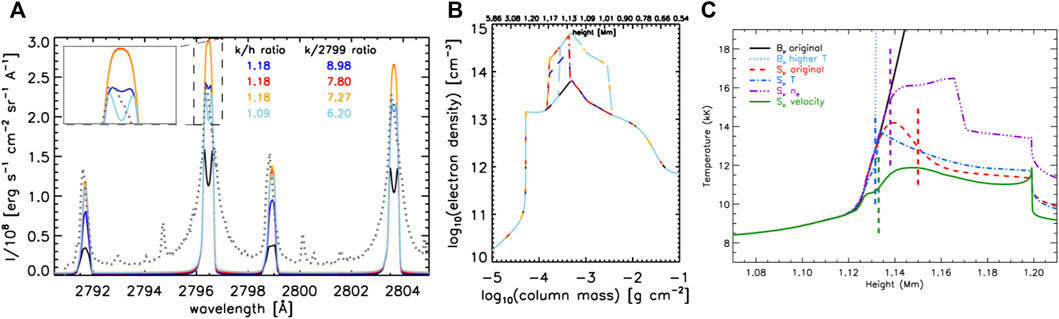
FIGURE 2. Illustrating the effect of increased electron density in the upper chromosphere on the Mg ii NUV spectrum. Panel (A) shows the Mg ii spectra synthesised from a RADYN simulation, using RH, where each colour represents a different modification to the electron density, the stratification of which is shown in panel (B). The black line is the original, and the dotted line is a sample observed flare spectrum from IRIS. The resonance to subordinate line ratios are indicated. An order of magnitude increase in the electron density to
Varying the temperature and electron density independently could not recover the very broad line wings. Instead, experiments with introducing extremely large downflows of v ∼ 200 km s−1 were attempted, in concert with weaker upflows v ∼ 75–100 km s−1. Combining unresolved flows did produce very broad resonance lines, but also too-weak subordinate lines. The blending of the far wings of the resonance lines with the quasi-continuum between them, and with the subordinate lines, was not well captured in those static models. While there is prima facie evidence from the modelling work of Rubio da Costa and Kleint (2017) that unresolved bi-directional flows can broaden the lines, my own opinion is that extreme macrovelocity ‘smearing’ of the lines is not the source of the missing widths far into the line wings. Such extreme flows are a difficult proposition. Downflows are typically modelled (and inferred from observations) as being much more modest, on the order of v ∼ a few× 10 km s−1, and concentrated in narrow, dense condensations. While complex flows often form in loop models, even sometimes with transient downflows of v ∼ 150 km s−1 in extended transition regions (e.g. Zhu et al., 2019), by the time the condensations reach the chromosphere they have cooled, accrued mass and decelerated to be v < 100 km s−1 (more often slower, to a few × 10 km s−1). That is not to say that extreme bi-directional flows are not what is happening in the actual chromosphere, but we therefore must determine a means to produce such large downflows in simulations that can capture the complex interplay between flows, the subsequent accrual and evacuation of mass, and the associated changes to opacity. One observational sanity check here could be to determine the k:h line ratio as a function of wavelength over the line, which may help determine the relative opacity of the secondary blueshifted component, which formed higher in the atmosphere.
To summarise, the experiments of Rubio da Costa and Kleint (2017) suggest that increasing the upper chromosphere temperature pushes the formation height of the Mg ii lines deeper, but that perhaps we are missing a temperature increase through the chromosphere to enhance the subordinate lines. The likely culprit behind filling in the central reversal is an enhanced electron density in the upper chromosphere, perhaps (in my view: certainly!) related to the dense condensations produced in RHD models and studied extensively by Prof. Kowalski and collaborators (see Paper 1). While extreme bi-directional velocity flows that are unresolved within an IRIS pixel appear to produce some of the missing line widths in their modelling, I am a bit more sceptical that these conditions can appear in the actual chromosphere. Rubio da Costa and Kleint (2017) clearly indicate that unresolved flows do play some role, but the flow magnitude required has not, to my knowledge, been inferred from typical observations of chromospheric spectral lines. A key focus for future flare modelling should be to 1) self-consistently combine several aspects of these important findings, e.g. a temperature rise through the lower-mid chromosphere would also raise the electron density and likely generate flows, and 2) to produce a flare model driven by some energy input that naturally produces the plasma conditions required by Rubio da Costa and Kleint (2017). We must also assess if the conditions that produce a closer match to Mg ii observations do not produce conditions that results in a discordant match to other spectral lines (e.g Hα, Ca ii 8,542 or Ca ii H and K).
One alternative potential resolution to the question of the missing line widths in the models is that we have been underestimating quadratic Stark broadening (electron pressure broadening). Though not terribly important for the Mg II NUV spectral lines in the quiet Sun, the many orders of magnitude enhancement of the electron density in flares could result in pressure broadening playing an outsized role10, due to the fact that quadratic Stark broadening is a function of the electron density. In RH the quadratic Stark effect is typically computed following classical Impact Theory with various approximations (see discussion in Zhu et al., 2019), including the adiabatic approximation. As Zhu et al., 2019 demonstrate, the adiabatic approximation is likely not valid for Mg ii. Instead, impact-semiclassical-theory provides a better estimate, which is included in the STARK-B database11. Zhu et al., 2019 modified RH to model Mg II Stark widths based on the STARK-B database, where the Stark width is a polynomial function of temperature and density. At the temperatures relevant for Mg ii the STARK-B results have an order of magnitude greater value than is typically modelled by RH. A RADYN simulation was produced with a very high peak electron beam flux of Fpeak = 5 × 10¹¹ erg s−1 cm−2, that was ramped up and down with FWHM of 20 s. Snapshots were processed through RH with and without the improved Stark broadening. The inclusion of increased Stark broadening resulted in broader profiles compared to the typical flare loop models (though only the h and k lines were strongly affected). Still, however, they remained too narrow compared to observations, and through experimentation it was found that a factor × 30 additional stark broadening was required over and above the STARK-B estimates to sufficiently broaden the lines. In that case, lines and quasi-continuum between the lines, were well reproduced, albeit with a factor
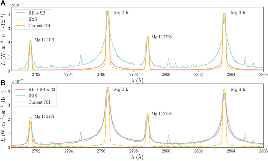
FIGURE 3. Improved treatment of Stark broadening for Mg ii lines results in broader line wings. (A) compares a RADYN simulation processed through RH, where yellow dot-dashed is the synthetic Mg ii line with standard Stark broadening, and the salmon coloured line is the line with improved Stark broadening of Zhu et al., 2019. The blue line is the observation, scaled in intensity. (B) illustrates that even with this improvement a further factor of ×30 Stark broadening would be required to produce a width consistent with the observation, indicating that we are still missing something in our models. Figure adapted from Zhu et al., 2019. © AAS. Reproduced with permission.
Additionally, single-peaked profiles were produced naturally by their model at several times. A detailed examination of the formation properties revealed that this happened when the electron density in the line formation region was exceptionally high (a result of the merging of several compressive flows), on the order of ne ≃ 8 × 1014 cm−3. The formation region was very narrow (Δz = 32 m, compared to Δz ∼ 100 s m at other times), with a constantly increasing temperature. These results confirmed the findings of Rubio da Costa and Kleint (2017) that the electron density in the formation region is a key factor in understanding the typically observed Mg ii lines. Zhu et al., 2019 also note that unresolved flows in their simulations did broaden lines, but not to the extent required as the flows had slowed to
There have been a few reports of blue wing asymmetries that are concentrated early in the development of flare sources (e.g., Kerr et al., 2015; Tei et al., 2018; Huang et al., 2019). A suggestion was put forward by Tei et al., 2018 that blue wing asymmetries at ribbon fronts were produced by gentle evaporation of cool, dense chromospheric material into the corona, ahead of a hot bubble of material. This cool material is heated and dissipates. They created a cloud model that could produce Mg ii h line blue wing asymmetries, along with the peak asymmetries observed. To my knowledge this has not been modelled in detail using flare loop models. A similar, but seemingly more extreme phenomenon, is the appearance of Mg ii profiles that have unique shapes that only appear in the leading edge of flare ribbons (so-called ribbon fronts), found by Xu et al., 2016 and Panos et al., 2018. As mentioned above, these exhibit quite different properties to brighter flare sources (namely blueshifted line cores, deep central reversals, and very broad profiles). When present, these profiles are located along the leading edge of propagating flare ribbons, and thus represent the very initial stages of energy deposition. Other ribbon front spectral behaviour includes the dimming of He i 10,830 Å before it brightens during the main part of the ribbons (e.g., Xu et al., 2016). Kerr et al. (2021) demonstrated using RADYN flare modelling that this dimming is caused by the presence of non-thermal particles in the chromosphere, and that a weaker flux with a harder distribution (that is, greater proportion of high energy electrons than low energy electrons) resulted in stronger dimming that was sustained for slightly longer. However, observed ribbon front behaviour can persist for up to 120–180 s (though they can also be shorter in duration), whereas the models of Kerr et al., 2021 predicted only a few seconds. Once the chromosphere was hot enough in those simulations, the He i 10,830 Å line was driven into emission. The causes of flare ribbon fronts (which do not appear uniformly along the ribbon), and how they transition to the more typical bright ribbons we have historically studied, is not known. Work is in-progress to address the ribbon front problem using RADYN modelling of electron beam driven flares: Polito et al., 2022 investigates the relation between the magnitude of energy flux deposited and response of the Mg ii ribbon front-like profiles, finding that weak energy fluxes are more consistent with ribbon-front like profiles and that stronger energy fluxes produce more ‘standard’ ribbon profiles. That study used the same simulations from Kerr et al., 2021, and those simulations that were most consistent with He i 10,830 Å ribbon front observations also resulted in Mg ii spectra that were comparable to ribbon-front observations. The implication here is that there are potentially different stages of energy deposition to explain the evolution from ribbon-front to ribbon spectral profiles, and follow on work from Polito et al., 2022, led by myself, is investigating how to obtain longer lived ribbon fronts in both He i and Mg ii. From these two on-going studies it is clear that the Mg ii ribbon front profiles can strongly constrain the characteristics of initial energy deposition into the chromosphere, and that high spatial-, temporal-, and spectral resolution observations in other wavelengths should focus on ribbon leading edges.
Prior EUV observations of hot flare lines have shown anomalously broad lines, of unknown origin (e.g., Milligan, 2011; Milligan, 2015). While several suggestions have been made, a definitive solution remains elusive (as you have no doubt realised by now, line widths are a sore spot for flare modellers). As discussed in Paper 1 in relation to probing the duration and magnitudes of chromospheric evaporation, the Fe xxi 1,354.1 Å line observed by IRIS offers a window at high spatial, temporal, and spectral resolution on hot flare plasma at
The Fe xxi 1,354.1 Å line has been observed in numerous flares by IRIS (e.g., Graham and Cauzzi, 2015; Polito et al., 2015; Polito et al., 2016; Young et al., 2015; Tian et al., 2015). It is observed to be largely symmetric, with significantly enhanced line widths. It is initially weak and broad, and becomes more narrow and intense over time. The line widths during flares have ranged from the instrumental + thermal width W ∼ 0.43 Å (assuming ionisation equilibrium) at loop tops to W ∼ [0.5–1] Å or larger in ribbons. Kerr et al., 2020 performed a superposed epoch analysis similar to Graham and Cauzzi (2015)’s Doppler shift analysis, to understand the typical evolution of Fe xxi line widths over time in the 2014-September-10th X-class flare. That event showed a large amount of scatter during the impulsive phase of the flare, but with W ∼ [0.6–1.2] Å, peaking after t ∼ 200 s, before gradually returning to pre-flare values over the subsequent 500 s or so.
A popular suggestion for the origin of the broad line profiles of hot lines is the superposition of flows along the line of sight from numerous Doppler shifted line components. Using the RADYN code, Polito et al., 2019 explored this idea. They produced several field-aligned flare simulations, with a t = 60 s heating duration. Synthetic Fe xxi emission was produced, with Doppler shifts applied as appropriate as a function of height along the loop. From those simulations they constructed both single and multi-stranded loop models, which for the latter had 100 identical threads each with a randomly selected start time within 15 s of the first thread start time. Other loop lengths and energy fluxes was also tested, but no change to the overall conclusions was found. The threads were then orientated in several ways that investigated the effects of loops being co-spatial or along a ribbon-like structure within 20 IRIS pixels, either aligned in the same angle or at different orientations. Emission from each set-up was summed to mimic different scenarios of IRIS looking through different lines of sight. Polito et al., 2019 found that there was a non-negligible asymmetry, with an anti-correlation between broadening and asymmetry (broader lines were more asymmetric), in contrast to observations which showed largely symmetric lines no matter the width, in each of their scenarios. Narrow profiles were quite symmetric, and were largely due to superposition of several upflows that had similar magnitudes, but the superposition of loops was unable to characterise the broad, symmetric Fe xxi profiles in this case. Figure 4 shows a sample of these experiments, for a single loop model with different orientations. The synthetic spectra and resulting broadening are shown, where it is clear that asymmetries are present.
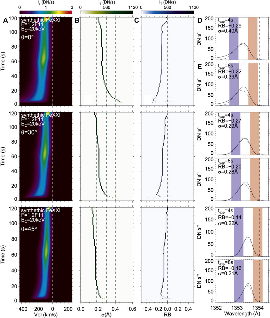
FIGURE 4. Synthetic Fe xxi 1,354.1 Å line profiles from a RADYN simulation that modelled the superposition of loops to attempt to explain line broadening. (A) shows the spectra as a function of time. (B) is the line width as a function of time, where the vertical lines are the minimum width (leftmost) and typical ranges from observations (two rightmost). (C) is the red-blue wing asymmetry as a function of time, where the horizontal line shows the typically observed values. (D–E) are synthetic spectra showing the difference in assumed exposure times. The coloured bands represent the areas used to calculate the red-blue wing asymmetry and the dashed curve is a single Gaussian fit to the spectra. The vertical line is the rest wavelength. The remaining panels show the same, but for different inclination angles of the loop to the solar surface. Figure adapted from Polito et al., 2019. © AAS. Reproduced with permission.
Kerr et al., 2020 also studied synthetic Fe xxi line widths using RADYN simulations. The model framework they developed, RADYN_Arcade, is described in Paper 1. From the field-aligned loops grafted onto the observed magnetic field skeleton, the superposition along the line of sight, and loop geometry was automatically taken into account. Qualitatively they produced synthetic Fe xxi emission that largely followed the observations. There was line broadening that was strongest at flare footpoints, and which narrowed along the loops towards looptops. However, while some profiles exceeded W ∼ 0.8 Å the majority of the Fe xxi lines only reached W ∼ [0.5–0.6] Å, much narrower than observed. There was not a very strong correlation between asymmetry and line width (broad profiles could be both symmetric or asymmetric), but the largest asymmetries were associated with the broadest profiles. The majority of the profiles were fit well with a single Gaussian, with only a subset requiring multiple components. There was also not a strong correlation between line width and Doppler shift, in contrast to some observations of hot flare lines studied by Milligan (2011). Finally, a synthetic superposed epoch analysis showed again a qualitative similarity to observations, but with profiles that were too narrow (with synthetic FWHM ∼ [0.4–0.8] Å, clustered around FWHM
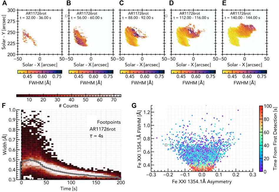
FIGURE 5. Evolution of Fe xxi widths in a RADYN_Arcade model. The top row (A–E) show maps of the line widths at various snapshots, illustrating that the footpoints and lower legs exhibit broader profiles. Taking all these pixels and producing a superposed epoch analysis (F) indicates that in comparison to an observations the line widths are too narrow. Panel (G) further illustrates that the profiles are too narrow, and that larger-than-observed asymmetries appear for some of the broadest profiles (colour represents elapsed time from the first moment that Fe xxi was detected in that pixel). Figure adapted from Kerr et al., 2020. © AAS. Reproduced with permission.
As set out nicely by Polito et al., 2019, there are several possible physical conditions that the RADYN modelling did not account for, which might explain how to obtain a closer match to the IRIS observations. Turbulence (including MHD wave turbulence) could broaden lines symmetrically. In fact, Allred et al., 2022 recently demonstrated that by suppressing thermal conduction in a RADYN simulation, via non-local effects or turbulence (e.g. Emslie and Bian, 2018), could lengthen the gradual phase of a flare, and produce a flow pattern more consistent with observations (e.g. Milligan and Dennis, 2009). Taking the turbulent mean free path of the best fit model, Allred et al., 2022 were able to estimate the broadening associated with turbulence for numerous lines (including hot lines from high charge states of Fe), finding that they were broadened substantially and symmetrically. There are plans to perform follow on studies to the modelling of Kerr et al., 2020, using these RADYN updates, and with the observed line widths from IRIS and the Hinode/EUV Imaging Spectrograph (EIS) observations as constraints on the degree of suppression to include. Using PREFT, Dr. William Ashfield and Dr. Dana Longcope are exploring the creation of MHD turbulence following loop retraction with added drag (private communication 2022). I eagerly await the application of their modelling to the formation of Fe xxi. Another source of broadening could be non-equilibrium effects, such that the ion temperature is very much larger than the equilibrium value of 11.2 MK. This would require an ion temperature on the order 40–60 MK, which also likely requires decoupling of the ion and electron temperatures (see also de Jager, 1985; Polito et al., 2018a). Given the high densities in flare footpoints, it is not clear if such extreme non-equilibrium processes apply, but the HYDRAD code is the ideal resource to study this in flares. Finally, Alfvénic waves propagating downwards from the magnetic reconnection site could broaden spectral lines via ion motions (see Section 3).
The extreme gradients through the transition region make it an important interface for mass and energy transport during flares. Strong lines produced in the transition region that are observed by IRIS are the Si iv and C ii resonance lines. Aside from study of their Doppler shifts, C ii has been relatively little studied in flare loop models. Si iv 1,394 Å and 1,402 Å, however, have been modelled in a few studies. I discuss their Doppler shifts in Paper 1, but here focus on their intensity ratio, and what that might tell us about temperatures and densities in the flaring transition region.
These lines have been used to infer flows in flares from their Doppler shifts, under the assumption that they are optically thin. They increase in intensity, broaden to a line width of similar magnitude to Mg ii, and exhibit red wing asymmetries indicative of mass flows on the order of a few ×10–100 km s−1 (e.g., Tian et al., 2015; Li et al., 2017; Yu et al., 2020). Non-Gaussian line shapes have been observed in flare ribbons, but most observations suggest optically thin formation from the ratio of the 1,394 Å/1,402 Å intensities (R1394∕1402 = 2; though it is often the case that only one of the lines is included in the IRIS lineslists), with exceptions discussed later in this section. Given the optically thin assumption, most flare modelling of this line was performed by computing the emissivity from CHIANTI atomic data alongside the stratification of physical variables from flare loop model atmospheres, and summing through height in some fashion to obtain the total intensity. However, some quiescent Sun studies suggested that effects of non-equilibrium radiation transfer, photoexcitation, or charge exchange may be important in setting the Si ion fraction stratification (e.g., Dudík et al., 2017; Dzifc̆áková et al., 2017; Dzifc̆áková and Dudík, 2018; Kerr et al., 2019c). Observations of line ratios in stellar flares have also suggested that the resonance lines of Si iv, and also of C iv, exhibit opacity effects (e.g., Bloomfield et al., 2002; Mathioudakis et al., 1999) and form under optically thick conditions, or, at least with some non-negligible optical depth τ > 0.1.
To determine the importance of radiation transfer effects on the formation of Si iv resonance lines during flares, Kerr et al., 2019c simulated a large number of electron beam driven flares using RADYN, and then generated the synthetic Si iv emission in two ways. The first was the standard optically thin synthesis using CHIANTI contribution functions and ionisation fractions, assuming equilibrium. The second was to use the minority species version of RADYN, MS_RADYN, to synthesise the two Si iv lines including the effects of photoionisation and photoexcitation, non-equilibrium ionisation, opacity, and charge exchange. MS_RADYN takes as input certain hydrodynamic variables at the cadence of RADYN′s internal timestep (i.e. the relevant timescales to capture dynamics, not simply the output cadence), and then solves just the NLTE non-equilibrium radiation transfer for a given minority species. That is, there is no feedback of the radiation from the minority species on the atmosphere itself. The line profiles from each method were quite different, even from the pre-flare where charge exchange broadened the Si iv ion fraction stratification, which peaked slightly cooler in temperature than it does in ionisation equilibrium (T ∼ 66 kK versus T ∼ 80 kK). Charge exchange is generally not considered in transition region line modelling, but both the results of Kerr et al., 2019c, and recent quiet Sun modelling of Dufresne et al. (2021a), Dufresne et al. (2021b) highlight its importance. Weaker simulated flares generally produced similar results from both synthesis methods. However, in stronger flares they differed. The peak intensities of MS_RADYN Si iv profiles were smaller, but the lines broader overall due to opacity effects so that the integrated line intensities were higher. Those profiles also showed stronger asymmetries, and self-absorption features. Crucially, the intensity ratio deviated from the optically thin ratio of R1394∕1402 = 2. Opacity effects were present in all simulations with an energy injection F > 5 × 10¹⁰ erg s−1 cm−2, and for some weaker flares with softer electron distributions since they more easily heated the upper chromosphere and lower transition region. Some of these flares only exhibited opacity effects for a transient period, since the transition region and upper chromosphere compressed quickly, meaning there was not a sufficient column mass of Si iv to build up opacity. When there was an extended flaring lower-transition region (that is temperatures climbing through 30 kK
There have since been a number of observations of R1394∕1402 deviating from the optically thin limit R1394∕1402 = 2 (e.g., Mulay and Fletcher, 2021; Zhou et al., 2022). Mulay and Fletcher (2021) found R1394∕1402 ≠ 2 at several locations along flare ribbons in an M7.3 flare. Zhou et al., 2022 report similar results, noting also that the ratio varies across the line profile, with stronger opacity in the core so that photons scattered from an optically thick core can easily escape through optically thin line wings. In those observations, we might infer that the flaring atmosphere produced the extended region of 40 < T < 100 kK at sufficiently high density. It is important to note that if we do not see much observational evidence for these potentially short lived opacity effects, then our models may be predicting too much density at these intermediate temperatures. Further RT modelling, particularly of other transition region lines in conjunction with Si iv is sorely required, as are high cadence observations to catch potentially transient opacity effects. Another impact of potential opacity effects in transition region lines, and motivation for their further study, is that these are important contributors to the (assumed) optically thin radiative loss functions, which are a major component energy loss in the simulations, governing the plasma response in our models.
Panos et al., 2021 and Panos and Kleint (2021) explored, using machine learning techniques based around mutual information theory (MI; Li, 1990)13, the correlation between the various spectral lines of IRIS through the transition region and chromosphere. I encourage the reader to read their detailed analysis carefully, in particular the subtleties surrounding selecting flaring areas and how this might impact correlations, but note the headline results here. They find weak correlations between spectral line pairs during quiescent periods, but substantially enhanced correlations of those pairs during solar flares. Mg ii and C ii have the strongest correlation, followed by their correlations with Si iv. Other lines (e.g. O iv) are more weakly correlated, and others such as Fe ii only show strong correlations directly over flare ribbons. This coupling meant that Panos and Kleint (2021) were able to predict the most probable spectrum of a certain IRIS observable given an input Mg ii spectra, for example. The strong correlation of Si iv to the chromospheric lines, despite the weak correlation of other transition region lines such as O iv, could be due to the deeper formation height suggested during the Kerr et al., 2019c simulations. Further, the coherency that flares introduce could be a result of the strong compression of the chromosphere and transition that occurs in many flare simulations. For example, Figure 11 in Kerr et al., 2019c shows that over time the range of formation height of the IRIS line cores can shrink to a very small Δz. The “big data” studies of Dr. Panos and collaborators provide an excellent test bed against which models can be critiqued—our models should be able to produce similar coherency between the various lines observed by IRIS, and this should be a target of our efforts in the near future.
Finally, I note briefly that it is typical in flare simulations from HYDRAD, RADYN, and FLARIX to produce large enhancements in electron density through the chromosphere and into the corona. These can be in excess of ne > 1013–14 cm−3 in the chromosphere, and ne > 1010–12 cm−3 through the transition region and lower corona. Indeed, as discussed in the preceding sections, a very large electron density at the Mg ii formation temperatures is required to explain the single peaked profiles. IRIS and Hinode/EIS density sensitive lines from the corona and transition region can demonstrate if these densities are consistent with observations. Polito et al., 2016 measured the ratio of the O iv 1,399.77 Å and O iv 1,401.16 Å line pair, which form at T ∼ 158 kK, during the impulsive phase of the X2-class flare that occurred on 2014-October-27th. The ratio reached the high-density limit, indicating that the density of the flare transition region reached ne > 1012 cm−3. A caveat here is the assumption of ionisation equilibrium, so that the observed ratio may be in part due to non-equilibrium effects. Other assumptions are that the lines are free of unknown blends, and that the plasma is a Maxwellian, which may not be the case in solar flares, or even active regions, which have been seen to exhibit κ distributions (e,g, Jeffrey et al., 2016; Dzifc̆áková et al., 2018; Del Zanna et al., 2022). Similar analysis using EUV spectral lines from EIS indicated a coronal density at 2 MK of ne > 1010–11 cm−3. Polito et al., 2016 then modelled this flare using HYDRAD, finding that the electron density in the synthetic flaring atmosphere (both flare footpoints and the transition region/lower corona) were consistent with the observationally derived values.
Pivoting slightly to white light observations, the IRIS NUV Balmer continuum modelling and observations seem to suggest that there is likely some contribution to the optical continuum excess in flares from recombination radiation in the upper chromosphere (see Section 3.3). Given the dependence of bound-free (and also free-free) emission on electron density, NUV and optical continuum observations of the chromosphere can give us some means to investigate the density there, and off-limb observations allow us to isolate the chromospheric portion. Off-limb observations of white light flares have revealed both the typical footpoint sources at the base of flare loops as well as bright loop structures (also referred to as prominence loop systems in some literature). The former was discussed by Heinzel et al., 2017, who analysed SDO/HMI continuum data of off-limb flares that revealed co-spatial HMI 6173 Å and RHESSI hard X-ray emission, with a characteristic height of
In this section I discuss how IRIS observations are aiding our efforts to not only refine and challenge the details of the electron beam model, but also in our efforts to explore additional energy transport mechanisms. Alternative mechanisms, that may act in concert with, or instead of, non-thermal electrons (likely varying in dominance in different spatial locations) that are under active study are: non-thermal protons or ions, downward propagating Alfvénic waves, and conductive heat flux resulting from direct in situ heating of the corona. There are possibly others too! I do not touch on non-thermal protons or heavier ions here, other than to say it that these accelerated ions are undoubtedly produced during solar flares and that they may carry energy equivalent to that of electrons (Ramaty and Mandzhavidze, 2000; Shih et al., 2009; Emslie et al., 2012; Aschwanden et al., 2017). That means we could be missing up to half of the energy delivered to the lower atmosphere in flares! Allred et al., 2020 recently updated the FP code, which has been merged with RADYN, to model the propagation of these suprathermal ions, and initial results have demonstrated that protons can penetrate much deeper into the lower atmosphere than electrons, aided by warm target effects (e.g., Allred and Kerr, 2021). I look forward to studies that use RADYN+FP proton-beam driven flares to forward model IRIS observables.
First proposed as a means of heating the temperature minimum region where non-thermal electrons likely could not reach, but which observational evidence suggested experienced a modest temperature rise in flares, Emslie and Sturrock (1982) constructed a simple but informative model of energy transport via downward propagating, coronally-generated, Alfvénic waves. In this model, waves would be produced from the reconnection site, propagating through the corona into the lower atmosphere to the temperature minimum region where they were damped by resistivity. These simulations assumed Mono-chromatic (single frequency) waves, employed the WKB approximation (that is, waves were not reflected by density gradients), and assumed an instantaneous travel time. These assumptions allowed a straightforward formulation of a damping length to model the dissipation.
This notion was revisited by Fletcher and Hudson (2008) who investigated the possibility that Alfvénic waves could not only deliver the energy liberated by magnetic reconnection to the chromosphere, and accelerate electrons in the corona via field-aligned electric fields but could also potentially locally accelerate electrons in the chromosphere via mode-conversion to high wave-numbers resulting in turbulent acceleration. More work is required to understand the role of these waves in particle acceleration. The thought experiments of Fletcher and Hudson (2008) explored Alfvénic waves as an alternative to the electron beam model as a means to deliver flare energy and explain observations of both hard X-rays and broadband enhancements of the UV/optical/infrared. This was motivated by perceived issues with the coronal acceleration problem, namely the vast numbers of electrons required (
Even if they are not required as a complete replacement to electron beams (which is still a source of vigorous debate), it is important that we continue to properly consider the role of Alfvénic waves in flares. Flares are, fundamentally, a violent restructuring of the magnetic field, meaning that MHD waves are undoubtedly produced. The question is, do they carry sufficient energy to play a non-negligible role in transporting energy compared to coronally accelerated electrons, and can they efficiently heat the chromosphere (either alongside or instead of those electrons). Additionally, we do not see hard X-rays all along the flare ribbons. Perhaps different parts of ribbons are heated by different mechanisms. Some MHD simulations by Russell and Fletcher (2013) and Russell and Stackhouse (2013) revealed that Alfvénic waves could penetrate the transition region density boundary if they had a high enough frequency, f > 1 Hz, meaning the WKB approximation could be used within loop models to further investigate high-frequency Alfvénic waves. They also noted that ion-neutral interactions were important, alongside electron resistivity, in damping the Alfvén waves.
Inspired by these results Reep and Russell (2016) modified HYDRAD to model Alfvén waves using the WKB approach of Emslie and Sturrock (1982), but with an updated treatment of damping which included ambipolar effects. Thus, the waves were damped by ion-neutral, neutral-electron, and electron-ion collisions. Modelling a range of Alfvén wave parameters, including the injected Poynting flux, mono-chromatic frequency, and wave number they found that they could strongly heat the chromosphere, and that they could drive explosive chromospheric evaporation. This model was further improved in HYDRAD by Reep et al., 2018b, to include the wave travel time, via ray-tracing so that the waves propagate at the local Alfvén speed. They show that in addition to certain wave parameters being damped more effectively in the lower atmosphere than in the upper chromosphere, that leading waves can effectively bore a hole through the chromosphere allowing following rays to penetrate deeper into the lower atmosphere. This occurred due to ionisation by the leading waves, reducing the local damping.
Following the approach of Reep and Russell (2016), Kerr et al., 2016 included Alfvén waves as a mode of energy transport into RADYN. This initial work employed the instant-travel approximation where the wave propagation was ignored. I have since updated RADYN to include the travel time of the wave in the same manner as Reep et al., 2018b. For the remainder of this section I mostly discuss the results using the Kerr et al., 2016 model, since those are the published results relevant to IRIS, but work modelling the IRIS observables including travel time is underway via both HYDRAD and RADYN.
Kerr et al., 2016 compared the atmospheric dynamics and radiative output of two RADYN simulations, 1) an electron beam, and 2) a mono-chromatic Alfvén wave. The energy flux of each was set to be 1 × 10¹¹ erg s−1 cm−2, and the Alfvén wave parameters set to most effectively heat the upper chromosphere. A magnetic field stratification was imposed for the purpose of defining the Alfvén speed and damping lengths; it did not evolve during the simulations. Two spectral lines were compared, the Ca ii 8,542 Å and Mg ii k line, the latter synthesised using RADYN atmospheres with RH. While the atmospheres showed some striking similarities in each model’s ability to heat the chromosphere and drive strong upflows, as was first seen in Reep and Russell (2016), there were intriguing differences in the chromospheric stratification. These differences revealed themselves in the spectral lines also.
The Alfvén waves produced a flatter, more spatially extended energy deposition profile compared to the electron-beam heating profile, resulting in temperature rises at deeper heights than the electron beam simulation. Despite this, it did take time for the electron density in the lower atmosphere to catch up to the electron beam simulation because of the absence of non-thermal collisional ionisation due to the beam itself. Runaway helium ionisation due to the more concentrated electron beam heating removed the 304 Å line as a radiator, resulting in a high temperature bubble forming, flanked by narrow cool high density regions. These flanking regions expanded as a high velocity upflow, and slower downflow (in addition to the initial explosive evaporation). While this did not form in the Alfvén wave simulation, a secondary upflow appeared in the Alfvén wave simulation also, but was more gentle with a shallower spatial gradient. In the electron beam simulation the Mg ii k line had a central reversal that was redshifted during most of the heating phase. The line wings had small optically thin contributions due to the flow patterns. In the Alfvén wave simulation, however, the line formed in a gentle upflowing region of the chromosphere, shifting the absorption profile strongly to the blue. Since the densities in the upflow were relatively weak this did not fully shift the line but instead pushed the core and blue k2v peak closer in formation height until they merged. The upflow produced optically thin contributions through the blue wing. Fewer absorptions due to shifting the absorption profile boosted the red k2r peak in comparison to the heavily suppressed k2v peak, meaning that the whole profile took on a very asymmetric form. The k line could be mistaken as being single peaked with a large blue wing asymmetry. Differences in the shape of the Mg ii k line cores were a direct result of the different flows, that themselves were due to the different stratifications of damping in either the electron beam or Alfvén wave energy transport mechanisms. Kerr et al., 2016 demonstrated that Mg ii can help discriminate between energy transport models, but much more work needs to be done here, particularly studying multiple IRIS spectral lines forming in a wider array of Alfvén wave driven simulations that include the wave travel time. The predictions from each model should also be compared to the k-means classifications of Panos et al., 2018, and we must work to improve the models to include a spectrum of wave frequencies, and to constrain the properties of the waves.
While Alfvén waves are certainly produced during magnetic reconnection they have been detected in situ in the magnetosphere, (e.g., Chaston et al., 2005; Wygant et al., 2002; Gershman et al., 2017), a vital question is how much energy do they carry to the lower atmosphere? Is it enough to compete with electron beams as an important contributor to the flare energy budget, or is it negligible and thus safely ignorable? Thus far, the simulations of Reep and Russell (2016), Reep et al. (2018b) and Kerr et al. (2016) injected a Poynting flux of the level that we know from electron beam driven flare simulations, and bolometric flare observations, is required to significantly heat the chromosphere. An observational constraint on the Poynting flux is required. An upper limit could be placed on this by investigating the width of lines formed at different temperatures (i.e., altitudes). The non-thermal component of the width could result from ion motion in response to an Alfvén wave. To demonstrate what the upcoming EUV observations from the Multi-Slit Solar Explorer (MUSE, scheduled for launch in 2026; De Pontieu et al., 2020) would reveal about solar eruptive events, many flare models synthesised MUSE observables and demonstrated how MUSE might discriminate between model predictions (Cheung et al., 2022). As part of that effort we modelled the broadening that would be induced due to an Alfvén wave propagating down the loops in our RADYN_Arcade model, noting that the line was indeed substantially broadened. This is demonstrated in Figure 6 which shows the RADYN_Arcade model before and after Alfvén wave broadening is included. Coordinated high spatiotemporal resolution observations between MUSE and the High Throughput EUV Solar Telescope (EUVST, also scheduled for a ∼2026 launch) could track the development of non-thermal widths during a flare, placing constraints on the Poynting flux. Knowledge of the coronal magnetic field would also be very advantageous here, to help set the Alfvén speed and damping lengths, and to determine the amplitude of magnetic field perturbations. Finally, it is worth noting that Alfvénic waves have been proposed as the mechanism responsible for the observed elemental fractionation between the photosphere and corona. Low-first ionisation potential (FIP;
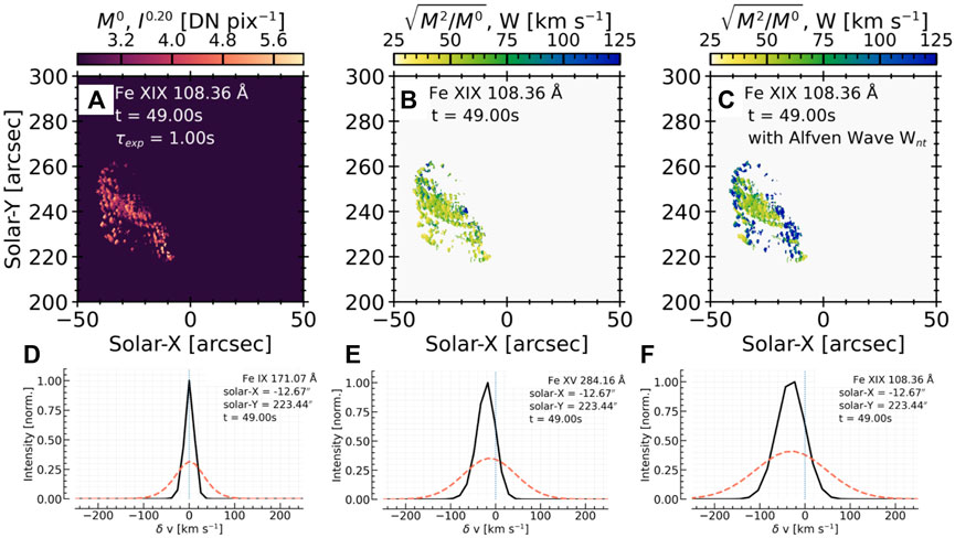
FIGURE 6. Demonstrating how Alfvén waves may explain some of the anomalous broadening of hot flare lines. In this RADYN_Arcade flare simulation predictions were made of the MUSE 108 Å line, forming at 10 MK. (A) shows the a map of the line intensity (zeroth spectral moment), scaled to the 1/5th power to show both weak and strong sources, at t = 49 s into the simulation, where hot footpoints and loop legs are apparent. (B) shows a map of the line widths (second spectral moment) where broadening is solely due to thermal and instrumental effects and the superposition of sources along the line of sight. (C) also shows a map of line width, but also includes broadening due to an Alfvén wave propagating along each loop, with a Poynting flux of 1×10¹⁰ erg s−1 cm−2 (a magnetic field was assumed for the purposes of calculating the Alfvén speed). Clearly the line was much broader. (D–F) show individual spectra, where black is the original, and the red-dashed is the Alfvén wave broadened version. Figure adapted from Cheung et al., 2022. © AAS. Reproduced with permission.
The energy flux injected to dynamic flare simulations has typically ranged on the order F = 109–11 erg s−1 cm−2, driven in part, admittedly, because of the computational expense and difficulty of injecting very much stronger values of F into time-dependent models until fairly recently (F > 1012 erg s−1 cm−2 fluxes, while computationally demanding, are now possible). This range has been inferred from numerous studies of flares in both the RHESSI era and before, but we are now realising that in some of the strongest flare sources we may be underestimating F, perhaps by an order of magnitude in some cases! The physical rationale and implications behind this, with regard to non-thermal particle production and transport, are beyond the scope of this review, but an important factor in tying down the existence of very high beam fluxes are the modern observations at high spatiotemporal resolution of UV and optical flare sources. IRIS, Hinode/Solar Optical Telescope (SOT), and ground based observatories have revealed flare sources are smaller that typically assumed from older data (particularly so if looking at white light flare data)14. A detailed study comparing source sizes from flare ribbons observed by Hinode/SOT to hard X-ray imaging spectroscopy suggested that the beam flux may very well be F > 1012 erg s−1 cm−2 in that flare (Krucker et al., 2011). Further, some groups have started looking at newly activated sources to define the areas into which energy is being injected within some observational window. Newly activated sources might be as small as to be on the order 1016 cm−2 or below (Krucker et al., 2011; Sharykin and Kosovichev, 2014; Milligan et al., 2014; Kleint et al., 2016; Kowalski et al., 2017; Graham et al., 2020). IRIS observations can both guide the magnitude to inject based on high resolution observations of source areas, and act as a validation.
Kowalski et al., 2017 injected fluxes of F = [1 × 10¹¹, 5 × 10¹¹] erg s−1 cm−2 to simulate the two brightest sources in the 2014-March-29th X-class flare, focussing on modelling the NUV continuum response. These fluxes were guided by the hard X-ray analyses of Kleint et al., 2016 and Battaglia et al., 2015, with the range based on arguments of the continuum emitting areas identified by Kowalski et al., 2017. Portions of the NUV continuum in the region λ ∼ [2,814–2,832] Å, observed by IRIS, were first identified by Heinzel and Kleint (2014), who extracted patches of continua free from lines. They determined these line-free regions as likely being part of the Balmer continuum that remained optically thin during the flare and which formed in the mid-upper chromosphere. This means the continuum response would be very sensitive to the electron density throughout the flare chromosphere. Kowalski et al., 2017’s numerical experiments showed that the NUV continuum was too weak in the lower energy flux simulation, and much too weak in a set of experiments in which similar energy flux was instead deposited directly in the corona and allowed to conduct down to the chromosphere (potentially due to the lack of non-thermal collisional ionisations in the conduction-only simulations, though this was not commented on by the authors). In the high energy flux simulation the continuum did reach a sufficient level to match observations by t ∼ 2 s, peaked a few seconds later, before declining thereafter (but still remaining 100–200% above the pre-flare). Thus, a high energy flux was in fact required to produce conditions to raise the continuum intensity to the observed level. An in-depth analysis found that the NUV continuum was formed by hydrogen recombination emission from two distinct layers, both optically thin: a stationary chromospheric layer and a dense condensation that rapidly forms and accrues mass. As time progressed the condensation became responsible for the bulk of the emission, due to the fact that as the density increased an increasing proportion of the non-thermal electrons thermalised in the condensation itself, and consequently the stationary layer cooled somewhat. The conditions inside this condensation were found to be comparable to those of earlier slab model explanations of Balmer continuum enhancements (e.g. Donati-Falchi et al., 1985), suggesting that condensations (and high beam fluxes) are required to explain the brightest continua enhancements.
Various effects should be accounted for when considering very large non-thermal electron flux densities, such as the beam-neutralising return current including the effects of runaways (Zharkova and Gordovskyy, 2005; Holman, 2012; Allred et al., 2020; Alaoui and Holman, 2017; Alaoui et al., 2021), and instabilities that affect the beam propagation (e.g. Hannah et al., 2009; Lee et al., 2008; Li et al., 2014). A discussion of those is included in Kowalski et al., 2017, but are beyond the scope of this review, though I note that the careful model-data analysis of the type performed by Kowalski et al., 2017 is crucial as we explore the impact of these effect in flare loop models.
In the standard flare model there is typically not enough power carried by the highest energy electrons to meaningfully heat the deepest chromospheric/photospheric layers. However, there are some strands of evidence that suggest we do indeed require heating deeper than models currently predict. Listing some examples: excess line widths of chromospheric transitions (e.g., Mg ii h and k) cannot be accounted for; there is evidence of heating at the temperature minimum region (e.g., from inversions of Mg i λλ4571Å and λλ5173Å, Metcalf et al., 1990a; Metcalf et al., 1990b); there is speculation that white light flares (WLFs) may originate from the photosphere via enhanced H− emission following a local temperature increase, or contain significant contributions from the lower atmosphere (see discussions in Neidig, 1989; Machado et al., 1989; Neidig et al., 1993; Martínez Oliveros et al., 2014; Kerr and Fletcher, 2014; Kleint et al., 2016; Jurc̆ák et al., 2018). An alternative explanation to the WLF problem is optically thin bound-free (recombination) radiation resulting from overionisation of the mid-upper chromosphere (e.g., Hudson, 1972). This would produce a Balmer jump at 3,646 Å. Of course, likely both of those mechanisms play a role. If we do need heating to great depth, then we must identify the agent capable of doing so, and constrain how much energy is required.
Given the scarcity of white light continuum observations, the NUV continuum as observed by IRIS is one such means to constrain the need for deep heating (the NUV is thought to be closely related to the optical continuum, albeit we do not yet know if they always originate from the same volume during flares). Heinzel and Kleint (2014) first determined that the Balmer continuum could be observed by IRIS, using observing windows in the NUV near λ = [2,813–2,816, 2,825–2,828, 2,831–2,834] Å. They carefully extracted narrow, line free, portions of the spectrum, finding
Following on from this initial detection, Kleint et al., 2016 studied the IRIS Balmer continuum emission alongside other continuum enhancements from both space and ground observatories, spanning the UV through infrared. They performed blackbody fits to data (including modifying the blackbody intensity due to opacity effects) to determine the viability of an upper photospheric origin to the continuum emission, finding that the NUV lay well above the blackbody curve predicted by the optical and IR emission (as expected if the NUV emission was indeed recombination radiation, producing a Balmer jump). Building upon the modelling work started by Heinzel and Kleint (2014), Kleint et al., 2016 selected a few models from Ricchiazzi and Canfield (1983) and calculated the non-LTE hydrogen recombination continuum using the MALI code. Several were consistent with the observed NUV continuum enhancements (with a non-thermal electron flux close to that derived from RHESSI observations for that flare), but those models under-predicted the optical and IR enhancements from SDO/HMI and the Facility Infrared Spectropolarimeter at the Dunn Solar Telescope (DST/FIRS). Instead, a semi-empirical model atmosphere with photospheric temperature rise was required to achieve consistency with the optical/IR observations. Finally, they manually modified atmospheres that were input to RH in an attempt to find a stratification consistent with all three regimes (UV, optical and IR). A model with a modest photospheric temperature increase alongside a strongly heated chromosphere was required, as shown in Figure 7. Thus, IRIS in combination with ground based observations demonstrated that in some events we may indeed need both chromospheric and photospheric heating. To my knowledge no time-dependent flare model has self-consistently produced such an atmosphere (electrons beams typically do not carry enough power to such depths), and this should be a focus of our continuing efforts. However, it should also be noted that since an optically thin source at T ∼ 10 kK produces optical emission with a radiation temperature of 4–6 kK (see e.g. Kowalski and Allred, 2018), some ambiguity remains. At the same time as attempting to model self-consistently the heating throughout the chromosphere and photosphere to determine how to obtain atmospheres similar to the empirical models of Kleint et al., 2016, we should endeavour to obtain IRIS observations in the NUV alongside a broad spectral coverage of the optical (e.g. from DKIST) to determine the spectral shape more accurately, which would help resolve the ambiguity over emission mechanisms.
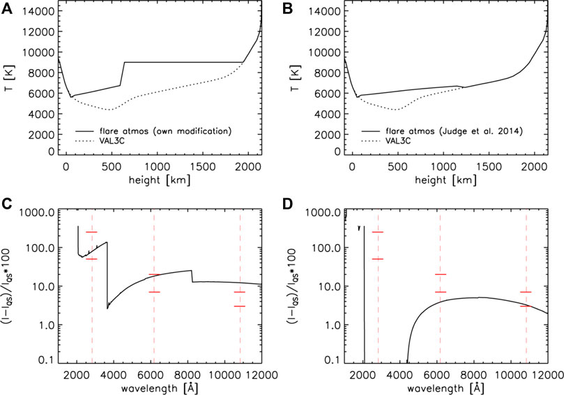
FIGURE 7. Synthetic continuum spectra from flare atmospheres processed using RH. Here Kleint et al., 2016 manually modified the temperature in the lower atmosphere to demonstrate that both a chromospheric temperature enhancement, and a temperature enhancement at greater depth (A) was required to synthesise the NUV and optical continuum (black line in (C)) that was consistent with the IRIS and SDO/HMI observations (red symbols on (C)). A lower atmosphere increase on its own (B) was not able to explain the Balmer continuum observations from IRIS (D). Figure adapted from Kleint et al., 2016. © AAS. Reproduced with permission.
Since it will likely remain challenging to obtain observations covering the Balmer jump (and thus a guide as to the formation of the optical continuum), Kowalski et al., 2019 have begun to search for alternative metrics that can gauge the extent to which the lower atmosphere is strongly heated. Using the fact that Fe ii lines observed by IRIS form under similar physical conditions as the NUV Balmer continuum (T ∼ 8–18 kK but mostly towards the cooler end, discerned from their earlier modelling work regarding high beam fluxes; Kowalski et al., 2017), they explored the ratio of wavelength-integrated flare excess Fe ii 2,814.45 Å intensity to the average continuum intensity in the region λ = [2,824.5–2,825.9] Å. This ratio was observed to be RFe:NUV ∼ 7–8 at the peak of very bright flare sources located in a sunspot umbra during the 2014-Oct-25th X class flare, significantly higher than the prediction from slab models with low-to-moderate densities of ρ < 10–9 g cm−3 which had values RFe:NUV ∼ 1. They speculate that this means there is significant heating (to T ∼ 10 kK) at high column depth (log m ∼ − 2 [g cm−2]) where Fe ii can be optically thick. They are currently modelling this ratio in a range of RADYN flares (private communication 2022), but noted that their earlier study of the 2014-March-29th X class flare (Kowalski et al., 2017) only produced an observed ratio of RFe:NUV ∼ 1, with a modelled ratio of RFe:NUV ∼ 1–1.8. Clearly there is something quite different at work during the 2014-Oct-25th flare. This could be due to the pre-flare atmospheres, since the 2014-October-25th flare sources propagated into the sunspot umbra, allowing a colossal 1,000% NUV contrast, and an excess intensity 20× that of the 2014-March-29th flare. Hopefully further observations from a variety of flares, and modelling of a variety of energy inputs (including varying the pre-flare atmosphere) will lead to a firm diagnostic of deep heating during IRIS flares.
The NUV continuum was forward modelled by Heinzel et al., 2016, using one of the short-pulse experiments of Kašparová et al., 2009. In those FLARIX simulations, a non-thermal energy flux was injected in a trapezoidal form over time, with peak flux F = 4.5 × 10¹⁰ erg s−1 cm−2. The whole pulse was very short, only lasting 3 s. The resulting Balmer continuum intensity was quite small compared to the observations of Kleint et al., 2016. This was attributed to the magnitude of energy flux deposited in the chromosphere. It was an order of magnitude smaller than that of the flare studied by Kleint et al., 2016. Further, the short duration of this relatively moderate injection meant that evaporation was weak and the pressure in the upper chromosphere did not increase to the level inferred from the best-match Ricchiazzi and Canfield (1983) analysed by Kleint et al., 2016. This could point to the need for either longer electron beam dwell times in large flares, or for a train of short pulses. In those models the hydrogen subordinate continua, in particular the Balmer continuum, were the dominant source of radiative losses throughout the chromosphere, overtaking losses from singly ionised metals such as Ca ii and Mg ii, underscoring the importance of IRIS Balmer continuum observations. Since the Balmer continuum is seemingly optically thin, the radiative losses integrated through the continuum formation heights are directly related to the emergent intensity. Thus, the observed excess intensities impose strict constraints on flare energetics.
The Balmer continuum is also a useful constraint for smaller events where heating is, largely, confined to the upper chromosphere. A ‘mini-flare’ event accompanying a jet was studied by Joshi et al., 2020 who determined that a reconnection event occurred at the base of the jet. A small Balmer continuum excess was present in very localised sources, from both IRIS SG spectra, and the SJI 2832 Å images (Joshi et al., 2021). Comparing to the analysis of Kleint et al., 2016, who had processed the Ricchiazzi and Canfield (1983) atmospheric models using MALI to obtain predictions for the hydrogen recombination continuum, Joshi et al., 2021 found that a few simulations were consistent with their observations. This balanced the continuum intensity, as well as the brightness of the Mg ii line cores. The most well matched models had non-thermal electron energy fluxes F = 1 × 10⁹–10 erg s−1 cm−2, with δ = 5 and Ec = 20 keV (note that the Ricchiazzi and Canfield 1983 did not sample other values of Ec and only a few values of δ for more energetic flares). From the Fermi/GBM (Meegan et al., 2009) hard X-ray observations, the injected non-thermal electron distribution was calculated as having an energy flux F = 6.5 × 10⁹ erg s−1 cm−2 for E > 20 keV, assuming the area into which the electrons were injected was the same as the continuum enhancement source. While there is some uncertainty in the low-energy cutoff, the parameters derived from the hard X-ray observations are consistent with those models that also provide a well-matched Balmer continuum excess intensity. Joshi et al., 2021 estimate that 82% of the intensity in the IRIS SJI 2832 Å images is continuum emission, contrasting the result from similar analysis of an X-class flare that found significant line emission (Kleint et al., 2017), which makes sense if we consider the weak energy flux involved that was unable to sufficiently excite the many lines within that part of the spectrum. In summary, small-scale reconnection at the base of a jet seemingly was able to accelerate enough electrons to bombard the upper chromosphere, enhancing the Balmer continuum, but was unable to really effect the lower chromosphere.
While there is unambiguous observational evidence for the presence of non-thermal electrons in a great many solar flares, they are not ubiquitously present. This is true both in the global sense, meaning there are some “thermal” flares that do not exhibit strong evidence of hard X-rays or microwaves of non-thermal origin, and the local sense meaning that hard X-rays sources do not appear uniformly along optical/UV flare ribbons (though this latter case may be related to the dynamic range of most hard X-ray observatories that precludes detection of weak sources alongside strong footpoints). In such flares in situ heating of the corona results in a conductive heat flux that transports energy to the lower atmosphere, generating the strong heating and mass flows (e.g. Zarro and Lemen, 1988; Battaglia et al., 2009; Fletcher et al., 2011; Brosius, 2012; Brosius and Holman, 2012; López et al., 2022). This is often referred to as ‘direct heating’, a somewhat nebulous term that refers generally to any heating of the corona (either looptops or along the legs of the loop) following the release of energy during magnetic reconnection15, including the retraction of magnetic loops that produce shocks such as those modelled by PREFT. It is indeed likely that some form of direct coronal heating acts alongside non-thermal electrons even in flares with clear evidence of particle acceleration, but the dominance of each mechanism varies from flare to flare and with spatial location. For example, recent results using GOES soft X-ray observations suggest that in a number of flares the corona is rapidly heated to T ∼ 10–15 MK before the onset of evaporation (so-called “hot onsets” Hudson et al., 2021). Several studies have either modelled flares as being purely driven by thermal conduction (e.g., Cheng et al., 1983; MacNeice, 1986; Gan et al., 1991, to name but a few) or have contrasted predictions between electron beam and conduction driven flares (e.g., Polito et al., 2018b; Kerr et al., 2021; Cheung et al., 2022). This latter exercise should be performed more often, as it is likely that both mechanisms act but the direct heating in the corona is often ignored. As shown in Cheung et al., 2022, the inclusion of direct heating can have impacts on the predicted intensities and Doppler motions of coronal and transition region lines. Some of those effects can only be seen at very high spatial and temporal resolution, such as will be afforded by the MUSE mission (see Section 4).
I summarise in detail here two recent examples of modelling flares driven purely by a conductive heat flux, and what we can learn about the nature of condensations from those simulations and IRIS observations.
The seminal studies of mass flows in flare models by Fisher et al. (1985a), Fisher et al. (1985b), and Fisher (1989) revealed the relationship between flare energy input and the development of both upflows and downflows in the chromosphere. Of those, Fisher (1989) concentrated on chromospheric condensations, developing an analytical model that described the timescales and magnitudes of flare-induced downflows. Fisher (1989) built that equation of motion from generalising various properties that occurred in flare loop models. Notably, Fisher, (1989) discovered that the lifetime of the condensations depend only on the chromospheric conditions, not the energy input, and is τlife ≈ 2(H/g)1/2, where H is the chromospheric density scale height and g is gravitational acceleration. For reasonable values of H, τlife ∼ 60 s. The half-life of the condensation was τ1/2 ≃ 2(H/g)1/2/Mpeak, where Mpeak is the ratio of the peak downflow velocity to the sound speed in the pre-flare chromosphere. Though τlife does not depend on properties of the energy injection, the peak downflow velocity (and thus τ1/2) does, varying as u0 ∝ F1/3, with some dependence on whether energy was transported via non-thermal electrons or was conducted down from a hot corona.
Ashfield and Longcope (2021) used the PREFT gas-dynamic code to study conduction-only driven chromospheric condensations, building upon and complementing the work of Fisher (1989). They found similar relationships, with some differences as described below, but using an alternative approach. They set up a simplified set of physical parameters to explore the dynamics of shocks in the chromosphere using jump conditions, and compared those predictions to numerical experiments. The analytical model informed a subsequent analysis and interpretation of numerical results from PREFT. Unlike Fisher (1989), Ashfield and Longcope (2021) allowed H to be a free parameter in their model, from which they found a similar scaling for the half-life, but with a different factor (2.8 versus 2). Casting in terms of u0 this was: τ1/2 ≈ 2.8H/u0. PREFT was set up as a rigid flux tube so that the only energy transport was via energy injected to the loop to mimic direct flare heating, and conduction-driven flares were simulated. Using those simulations with various values of pre-flare H and injected energy flux F, the velocity as a function of time u(t) was fit with a similar functional form as that from their analytical model. The best-fit values suggested that the relationship was instead τ1/2 ≈ 1.67H/u0, with the discrepancy attributed to at least one of the simplifying assumptions in their analytical model not being satisfied. The results of Fisher (1989) and Ashfield and Longcope (2021) demonstrate that both analytically and numerically the pre-flare chromospheric density scale height H ∝ u0τ1/2, with the numerical results of Ashfield and Longcope (2021) pointing to H ≃ 0.6u0τ1/2. The slight difference between the results of Ashfield and Longcope (2021) and the earlier work of Fisher (1989) could be due in part to the heating profile assumed. Fisher (1989) assumed short pulses of non-thermal electrons in the models which the analytical expressions used a base, whereas Ashfield and Longcope (2021) assumed direct heating in the corona. Nevertheless, this is a rather powerful diagnostic that suggests variations in the lifetime of condensations could be related to variations in the pre-flare chromospheric densities into which shocks propagate, and that variations along a flare ribbon could reveal corrugation of the pre-flare atmosphere. Note that the condensations referred to here are the relatively strong, transient, downflows that may appear on top of a longer-lived envelope as discussed Paper 1. The peak velocity, u0, itself scaled with the input energy flux, without much reliance on H, going as u0 ∝ F1/2 for weaker energy fluxes (F < 2 × 10¹⁰ erg s−1 cm−2), and u0 ∝ F1/3 for stronger fluxes. The latter was predicted by Fisher (1989), and the former by Longcope (2014) for low-energy fluxes.
Applying their findings to an actual flare, Ashfield et al., 2022 analysed the 2014-October-25th X-class event. During the flare there were persistent redshifts of Si iv, with vDopp ∼ 10 km s−1, but on top of which were many transient (
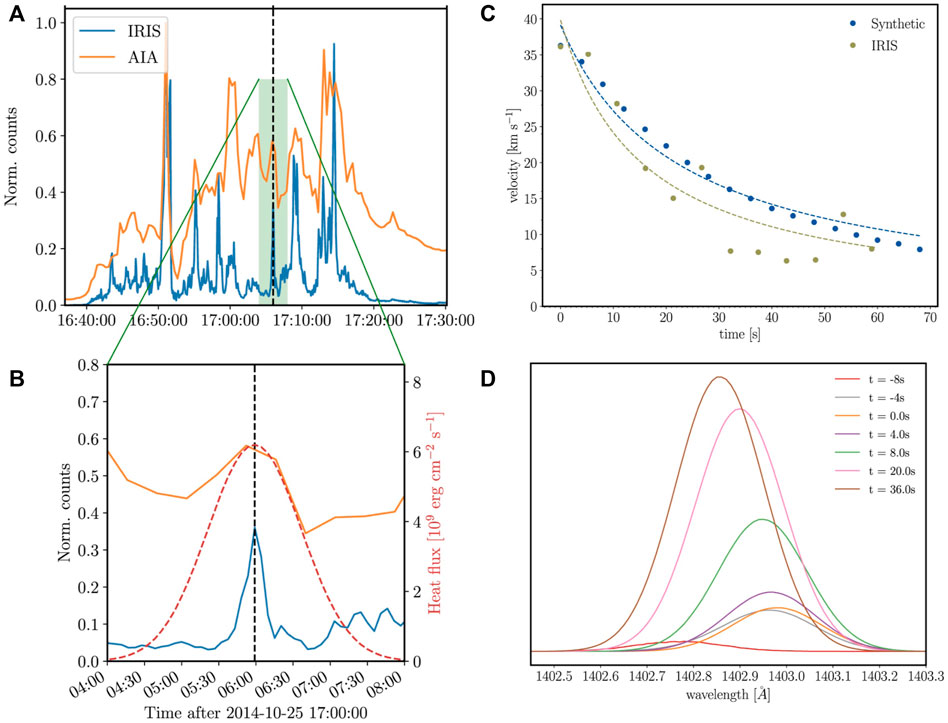
FIGURE 8. A thermal conduction driven flare simulation using PREFT. (A) shows observations of a single pixel in the 2014-Oct-25th X class flare. The Si iv 1402 line lightcurve is shown in blue, and the SDO/AIA 1600 Å lightcurve is shown in orange. The dashed line shows the peak of the individual condensation event studied. (B) shows a zoomed in view, where the injected heat flux is shown also, which was derived via the UFC method (red, dashed line). The resulting Si iv redshifts due to the condensation are shown in (C) where blue symbols are the PREFT results and green are the IRIS observations of that pixel. The dashed lines are fits to the decay of the condensation according to the model described in Ashfield and Longcope (2021). (D) shows the synthetic line profiles on an arbitrary intensity axis. Figure adapted from Ashfield et al., 2022. © AAS. Reproduced with permission.
Injecting this derived energy flux profile into the PREFT loop resulted in the formation of a condensation, peaking prior to the peak of the energy input, and reaching a maximum of velocity 45 km s−1, before decreasing to 10 km s−1, again prior to the peak energy input. Only a small fraction of the input energy flux was required to drive the condensation, leading to the conclusion that the timescales of condensations do not necessarily impart knowledge of the duration of energy input, in agreement with the analytical work of Fisher (1989). From the dynamic PREFT simulation, the Si iv spectral lines were synthesised assuming optically thin emission, and summed through the extent of each leg of the loop. Non-equilibrium effects were considered by tracking the change in ionisation state for each Lagrangian grid cell. While qualitatively consistent with the observed Si iv emission from the footpoint, with similar redshifts produced (see the righthand column of Figure 8), the synthetic intensities did not track the condensation evolution and were over an order of magnitude too high. The synthetic profiles were also fully redshifted rather than showing two component behaviour, possibly pointing to the need for many strands along the lines of Reep et al., 2018a’s multi-threaded modelling. Since the synthetic profiles continued to increase in intensity after their peak redshift, it is possible that the Gaussian form assumed for energy input was not correct. Keeping the total energy from the UFC method, but having a more impulsive initial energy release could decrease the energy deposited later in the event, reducing the line’s intensity. Prior experiments with PREFT that included the loop retraction exhibited much more rapid energy release (Longcope and Klimchuk, 2015). Of particular importance here, aside from testing the work of Ashfield and Longcope (2021), and demonstrating that the observed conductions could be produced in a thermal conduction-driven flare, was that this was the first simulation of a flare in which the energy input to the chromosphere was inferred from coronal observations.
In this extensive review (including Paper 1) I have illustrated how the powerful combination of high spatial-, temporal-, and spectral-resolution observations of the chromosphere, transition region and corona, coupled with state-of-the-art numerical loop models can greatly further our understanding of the physics of solar flares. IRIS observations have been used to challenge the predictions of models, requiring us to update the physics we include in our models, as well as the ways in which we perform model-data comparisons. The models, on the other hand, have been used to assist in the interpretation of IRIS observations, particularly of the complex formation properties of the optically thick chromospheric and transition region spectral lines. Through study of Doppler shifts and line asymmetries, both their magnitude and lifetimes, we have come to understand the likely requirement of muti-threaded modelling to understand upflows. Chromospheric condensations, on the contrary, seemingly do not require multi-threaded modelling, presenting a discrepancy. Detailed comparisons of synthetic optically thick lines, and the NUV and optical continua, have demonstrated that while flare models can capture the upper chromospheric response to flare energy injection, we are perhaps missing heating deeper in the atmosphere. If higher energy fluxes are required, as suggested by some model-data comparisons, do those originate solely from non-thermal electrons or do we need other agents by which flare energy can be transported to the chromosphere? We must seriously consider Alfvénic waves, and non-thermal ions, and work to characterise the magnitude of energy directly deposited into the corona that is subsequently conducted down. Recent model improvements have included incorporating area expansion and suppression of thermal conduction, but more work on those features is required in particular to tie down the appropriate parameter spaces to use in general flare models (e.g. when producing grids of models). Modelling IRIS observables has also revealed that opacity effects could occur for transition region lines, which are important contributors to the “optically thin” radiative loss functions in the models. A re-evaluation of the loss tables would be a worthwhile enterprise considering their importance, with HYDRAD NEI results helping to assess which species are also likely to suffer from non-equilibrium effects.
There still remain open questions, likely pointing to missing ingredients in our models. While they are many, I take the liberty to note the questions that capture my own focus at the present moment: 1) What causes the very broad chromospheric spectral lines? Could this point to the need for deeper heating through the lower atmosphere, and if so what transports that energy? 2) What is the nature of white light flares? Are they largely of chromospheric origin like the Balmer continuum that IRIS has observations have suggested, or do we need additional heating through the lower atmosphere? 3) What is the source of post-impulsive phase energy transport that maintains the flare gradual phase? 4) What is the nature and magnitude of turbulence throughout the flaring atmosphere? Turbulence could explain broadening of coronal lines and the suppression of thermal conduction, as well causing heating in its own right and particle acceleration. Continued coupling of flare loop modelling and high quality observations, can help address, and close, these questions. A powerful method to both guide and evaluate the models is the atmospheric stratification obtained from spectral inversions, for example using the IRIS2 database of Mg ii inversions (Sainz Dalda et al., 2019) and subsequent updates to further constrain the atmospheres using other IRIS lines. These should be compared to the output of flare models, with the results of both critically compared and interrogated to determine when they agree, when they disagree and in that event, crucially, why they disagree.
IRIS continues to deliver excellent observations. Both from observational analysis, and from numerical modelling it has become clear that flare processes can occur at rapid cadence, on the order of seconds to sub-second. In the present solar cycle there will be concerted efforts to obtain flare observations of the main IRIS lines (Mg ii k, Si iv 1,402 Å, C ii resonance lines, and sometimes O i 1,356 Å) with very high cadences of t < 1.5 s or even at sub-second cadence. This observing campaign has already caught many flares16. Additionally, we can look ahead to future missions that build upon the heritage of IRIS, both technologically and from the methodological approach of strongly coupling modelling and observations. Those missions include the Solar-C EUV High-Throughput Spectroscopic Telescope (EUVST; Shimizu et al., 2019), and the Multi-slit Solar Explorer (MUSE; De Pontieu et al., 2020). EUVST is a single-slit spectrometer with a huge temperature coverage spanning the chromosphere through hot flare plasma (T = 0.02–15 MK), observing with spatial resolution of 0.4 arcsec and temporal resolution down to
At the same time as obtaining ever higher quality observations we must strive to improve our modelling ability and frameworks. To make rapid and serious progress not only in solar flare physics, but in modern space physics more generally, we must have significant investment of time and resources in models. This involves continued improvements of our existing field-aligned models (some examples are discussed in Section 5.2 of Kowalski et al., 2022), but also to attempt to bridge the gap to multi-dimensional models. A fully 3D radiative-MHD model capable of simulating an NLTE chromosphere to sub-metre scales following flare energy injection is a daunting task that may not be fully realised for many years, but certainly we must attempt to include multi-dimensional effects. Efforts are already underway to study 2D/3D RT effects. For example, Osborne and Fletcher (2022) are exploring the effects of 2D radiation transfer, using 1D field-aligned RADYN models embedded within regions of quiet-Sun, finding significant differences may be present (including on the intensity of transition region lines, private communication). Additionally, non-thermal electrons have now been included in 3D radiative-MHD simulations, with very low fluxes to explore nano-flare heating (Bakke et al., 2018), and hopefully larger fluxes typical of flares may be explored in the future. However, we must also think about how to handle horizontal expansion of plasma in flare footpoints in the field-aligned models that can handle the vertical scales required in the chromosphere.
Recently, Dr. Joel Allred and co-authors proposed an end-to-end modelling framework of solar eruptive events in a white paper titled “Next-Generation Comprehensive Data-Driven Models of Solar Eruptive Events” 17 submitted to the National Academy of Science Solar and Space Physics Decadal Survey. In this framework, models that target different aspects of solar eruptive events should be linked such that the output of one is either the input to the next link in the chain, or strongly guides/constrains the next link, ideally in a data-driven or data-constrained manner. Field-aligned models would be an essential component. An example of such a chain could be: 1) an MHD model of the build up and release of magnetic energy, that then drives 2) a model of particle acceleration, the energy spectrum of which drives, 3) a model that propagates and dissipates non-thermal particles, producing 4) the radiative hydrodynamic response of the atmosphere, that 5), ultimately predicts observables, including geometry of the original magnetic field/loops (e.g., via a RADYN_Arcade type framework). The latter three steps are of course already being done with the models discussed in this review (e.g., RADYN + FP). Joined up modelling such as that described by Allred et al., interrogated by high-resolution observations, is perhaps the best way to make rapid progress whilst covering the vast range of scales, from MHD to kinetic, present in solar flares.
GK performed the literature review and wrote the manuscript.
GK acknowledges funding via a NASA ROSES Early Career Investigator Award (Grant# 80NSSC21K0460), and the Heliophysics Supporting Research program (Grant# 80NSSC21K0010).
IRIS is a NASA small explorer mission developed and operated by LMSAL with mission operations executed at NASA Ames Research center and major contributions to downlink communications funded by the Norwegian Space Center (NSC, Norway) through an ESA PRODEX contract. This manuscript benefited from discussions held at a meeting of International Space Science Institute team: “Interrogating Field-Aligned Solar Flare Models: Comparing, Contrasting and Improving,” led by GK and V. Polito. I also thank the following colleagues for their help, and patience, with answering questions related to RADYN, PREFT, FLARIX, and HYDRAD: Joel Allred, Mats Carlsson, Adam Kowalski, Vanessa Polito, Dana Longcope, William Ashfield, John Unverferth, Stephen Bradshaw, Jeffrey Reep, Jana Kašparová, Petr Heinzel, and Michal Varady. Finally, I thank the referees for their diligent reading and useful comments which improved both content and clarity of this review.
The author declares that the research was conducted in the absence of any commercial or financial relationships that could be construed as a potential conflict of interest.
All claims expressed in this article are solely those of the authors and do not necessarily represent those of their affiliated organizations, or those of the publisher, the editors and the reviewers. Any product that may be evaluated in this article, or claim that may be made by its manufacturer, is not guaranteed or endorsed by the publisher.
1Though ions likely carry significant amounts of energy (e.g., Emslie et al., 2012), the flare community primarily considers electrons since their signatures are easier to infer from hard X-rays. Flare accelerated protons and heavier ions are harder to constrain with current observational capabilities.
2https://github.com/solarFP/FP.
3RADYN and FLARIX currently uses CHIANTI V8, and HYDRAD V10, but the version should be noted in the relevant studies.
4As stated in Paper 1: CRD assumes that the wavelength of a scattered/emitted photon is uncorrelated to the wavelength at which it was absorbed, due to collisions (e.g., photons absorbed in the line wings may be redistributed and emitted at a wavelength in the line core). However, in relatively low-density environments such as the chromosphere there may be an insufficient number of elastic collisions such that the scattered photon has a wavelength that is correlated to that of the absorbed photon. Photons absorbed in the line wings are re-emitted in the wings, where it easier to escape. This is the partial frequency redistribution (PRD) scenario. CRD has a frequency independent source function, whereas PRD has a frequency dependent source function and the absorption profile does not equal the emission profile. See discussions in Hubený (1982), and Uitenbroek (2001), Uitenbroek (2002).
5This is typically the integrated intensity, but recently Zhou et al., 2022 showed in their study of the Si iv resonance lines it can be instructive to consider the ratio as a function of wavelength.
6https://star.pst.qub.ac.uk/wiki/public/solarmodels/start.html.
7The line source function is, roughly, a measure of the ratio of the upper and lower level populations, which depends on local conditions via collisions, and non-local conditions via the radiation field. The dominance of radiative processes over collisions, and the escape of radiation near τλ = 1, means that the source function deviates from the Planck function. In fact, this is what creates the central reversal in optically thick lines. While the Planck function increases with height due to larger temperatures, the source function decreases as it deviates from the Planck function. The line core source function is smaller at the height where the line core k3 photons can escape (z(τλ,core = 1)) than the source function at a deeper altitudes where the photons that create the flanking k2 peaks escape (z(τλ,k3 = 1) > z(τλ,k2 = 1)). Increasing collisions (e.g., via a larger density and temperature) helps to maintain or increase the population of the upper level via collisional transitions, and the source function more closely tracks the local Planck function, reducing the difference between the k2 and k3 source functions, such that the central reversal can reduce in depth or disappear.
8Temperatures originally climbed from log10T ∼ 4.1 [K] to log10T ∼ 4.6 [K] between column mass of log10 ∼ [−3.6, −4.3] [g cm−3], before then rapidly attaining transition region/coronal temperatures a column mass of log10 > − 4.4 [g cm−3]. They were modified to instead increase from log10T ∼ 4.1 [K] to log10T ∼ 4.9 [K] at a column mass of log10 ∼ [−3.4, −3.6] [g cm−3], before more gradually increasing to log10T > 5.5 [K] between column mass of log10 = [−3.6, −4.3] [g cm−3].
9Roughly, increasing the electron density by an order of magnitude though column masses of log10 ∼ [−3.6, −3.8] [g cm−3], peaking at log10ne ∼ 14.8 [cm−3].
10Note that this is in contrast to the lower density flaring corona and transition region. Milligan (2011) found that pressure broadening played a negligible role in the broadening of optically thin lines in the corona and transition region.
11A database of Stark widths for various atoms/ions: http://stark-b.obspm.fr/.
12This intensity discrepancy is likely a combination of the atmospheric stratification, and other factors such as 3D radiation transfer and the assumed filling factors of the observations. While this is a large intensity offset, such exploratory studies of chromospheric observables still teach us about important physical processes, even if we do not yet simultaneously solve both the problem of intensity and broadening here.
13MI captures statistical dependencies, in this case between various features of different spectral lines. If the information in one spectral lines is independent from the other spectral line, the joint probability of obtaining a certain property of line X alongside a property of line Y is the product of the individual probabilities. If however the probabilities are related due to some correlation between the properties of lines X and Y then the joint probability is a more complicated evaluation. The specific elements of “information” are many and varied (for example the probability that a Mg ii line has a single peak or central reversal at the same time that Si iv is doppler shifted). As applied by Panos et al., 2021 and Panos and Kleint (2021) MI aggregates the many properties and outputs a single score that describes how correlated the lines appear to be overall, which can be studied spatially and temporally.
14An assumption here is that the white light flare area represents the same area into which electrons are deposited. While the hard X-ray sources sizes are large due to the relatively poor spatial resolution of those instruments, we do not know with certainty that the small white light areas represent the true areas from which hard X-rays originate. There is some ambiguity as to the relative heights at which hard X-rays and white light emission is produced, though as we will see models do suggest they are close. Observations of limb flares also suggest that some white light emission and the hard X-rays come from the same volume (e.g., Krucker et al., 2015). Additionally, there could be area expansion through the loop affecting source areas. All this is to say that while we now believe that white light and UV source areas are truer representations of the area into which non-thermal electrons are deposited, it is perhaps best to say that they are a lower limit, with the upper limit coming from the hard X-rays.
15This does not include potential heating of the corona by very low-energy non-thermal electrons that are thermalised in the lower corona, which are already captured by the models. In such cases, a conductive heat flux is present due to this coronal heating, but in this section we refer to coronal heating in flares in the absence of non-thermal particles.
16https://iris.lmsal.com/data.html.
17White papers will appear in the Bulletin of the American Astronomical Society, but are for now hosted by the NAS on their website: https://www.nationalacademies.org/our-work/decadal-survey-for-solar-and-space-physics-heliophysics-2024-2033. A link to Dr. Allred’s white paper is: http://surveygizmoresponseuploads.s3.amazonaws.com/fileuploads/623127/6920789/140-a8d175a52b5836b620abf6d961febf97_AllredJoelC.pdf.
Abbett, W. P., and Hawley, S. L. (1999). Dynamic models of optical emission in impulsive solar flares. Astrophysical J. 521, 906–919. doi:10.1086/307576
Alaoui, M., Holman, G. D., Allred, J. C., and Eufrasio, R. T. (2021). Role of suprathermal runaway electrons returning to the acceleration region in solar flares. Astrophysical J. 917, 74. doi:10.3847/1538-4357/ac0820
Alaoui, M., and Holman, G. D. (2017). Understanding breaks in flare X-ray spectra: Evaluation of a cospatial collisional return-current model. Astrophysical J. 851, 78. doi:10.3847/1538-4357/aa98de
Allred, J. C., Alaoui, M., Kowalski, A. F., and Kerr, G. S. (2020). Modeling the transport of nonthermal particles in flares using fokker-planck kinetic theory. Astrophysical J. 902, 16. doi:10.3847/1538-4357/abb239
Allred, J. C., Hawley, S. L., Abbett, W. P., and Carlsson, M. (2005). Radiative hydrodynamic models of the optical and ultraviolet emission from solar flares. Astrophysical J. 630, 573–586. doi:10.1086/431751
Allred, J. C., Kerr, G. S., and Gordon Emslie, A. (2022). Solar flare heating with turbulent suppression of thermal conduction. Astrophysical J. 931, 60. doi:10.3847/1538-4357/ac69e8
Allred, J. C., Kowalski, A. F., and Carlsson, M. (2015). A unified computational model for solar and stellar flares. Astrophysical J. 809, 104. doi:10.1088/0004-637x/809/1/104
Allred, J., and Kerr, G. (2021). “Modeling the transport and heating resulting from nonthermal ions in solar flares,” in AGU Fall Meeting Abstracts, SH24B–04.2021
Aschwanden, M. J., Boerner, P., Ryan, D., Caspi, A., McTiernan, J. M., and Warren, H. P. (2015). Global energetics of solar flares: II. Thermal energies. Astrophysical J. 802, 53. doi:10.1088/0004-637X/802/1/53802
Aschwanden, M. J., Caspi, A., Cohen, C. M. S., Holman, G., Jing, J., Kretzschmar, M., et al. (2017). Global energetics of solar flares. V. Energy closure in flares and coronal mass ejections. ApJ 836, 17. doi:10.3847/1538-4357/836/1/17
Ashfield, I., William, H., Longcope, D. W., Zhu, C., and Qiu, J. (2022). Connecting chromospheric condensation signatures to reconnection-driven heating rates in an observed flare. Astrophysical J. 926, 164. doi:10.3847/1538-4357/ac402d
Ashfield, W. H., and Longcope, D. W. (2021). Relating the properties of chromospheric condensation to flare energy transported by thermal conduction. Astrophysical J. 912, 25. doi:10.3847/1538-4357/abedb4
Bakke, H., Frogner, L., and Gudiksen, B. V. (2018). Non-thermal electrons from solar nanoflares. In a 3D radiative MHD simulation. Astronomy Astrophysics 620, L5. doi:10.1051/0004-6361/201834129
Battaglia, M., Fletcher, L., and Benz, A. O. (2009). Observations of conduction driven evaporation in the early rise phase of solar flares. Astronomy Astrophysics 498, 891–900. doi:10.1051/0004-6361/200811196
Battaglia, M., Kleint, L., Krucker, S., and Graham, D. (2015). How important are electron beams in driving chromospheric evaporation in the 2014 march 29 flare? Astrophysical J. 813, 113. doi:10.1088/0004-637x/813/2/113
Bloomfield, D. S., Mathioudakis, M., Christian, D. J., Keenan, F. P., and Linsky, J. L. (2002). Opacity in the upper atmosphere of AU Mic. Astronomy Astrophysics 390, 219–224. doi:10.1051/0004-6361:20020690
Bradshaw, S. J., and Mason, H. E. (2003a). A self-consistent treatment of radiation in coronal loop modelling. Astronomy Astrophysics 401, 699–709. doi:10.1051/0004-6361:20030089
Bradshaw, S. J., and Mason, H. E. (2003b). The radiative response of solar loop plasma subject to transient heating. Astronomy Astrophysics 407, 1127–1138. doi:10.1051/0004-6361:20030986
Brosius, J. W. (2012). Extreme-ultraviolet spectroscopic observation of direct coronal heating during a C-class solar flare. Astrophysical J. 754, 54. doi:10.1088/0004-637x/754/1/54
Brosius, J. W., and Holman, G. D. (2012). Using SDO’s AIA to investigate energy transport from a flare’s energy release site to the chromosphere. Astronomy Astrophysics 540, A24. doi:10.1051/0004-6361/201118144
Brown, J. C. (1971). The deduction of energy spectra of non-thermal electrons in flares from the observed dynamic spectra of hard X-ray bursts. Sol. Physcs 18, 489–502. doi:10.1007/bf00149070
Canfield, R. C., and Chang, C. R. (1985). Ly-alpha and H-alpha emission by superthermal proton beams. Astrophysical J. 295, 275–284. doi:10.1086/163371
Canfield, R. C., and Gayley, K. G. (1987). Impulsive H alpha diagnostics of electron-beam–heated solar flare model chromospheres. Astrophysical J. 322, 999. doi:10.1086/165795
Canfield, R. C., Gunkler, T. A., and Ricchiazzi, P. J. (1984). The H-alpha spectral signatures of solar flare nonthermal electrons, conductive flux, and coronal pressure. Astrophysical J. 282, 296–307. doi:10.1086/162203
Canfield, R. C., and Ricchiazzi, P. J. (1980). A probabilistic approach to radiative energy loss calculations for optically thick atmospheres - hydrogen lines and continua. Astrophysical J. 239, 1036–1044. doi:10.1086/158193
Canfield, R. C., Wulser, J.-P., Zarro, D. M., and Dennis, B. R. (1991). A study of solar flare energy transport based on coordinated H alpha and X-ray observations. Astrophysical J. 367, 671. doi:10.1086/169663
Carlsson, M., and Leenaarts, J. (2012). Approximations for radiative cooling and heating in the solar chromosphere. Astronomy Astrophysics 539, A39. doi:10.1051/0004-6361/201118366
Carlsson, M., Leenaarts, J., and De Pontieu, B. (2015). What do IRIS observations of Mg II k tell us about the solar plage chromosphere? Astrophysical J. Lett. 809, L30. doi:10.1088/2041-8205/809/2/L30
Carlsson, M., and Stein, R. F. (2002). Dynamic hydrogen ionization. Astrophysical J. 572, 626–635. doi:10.1086/340293
Carlsson, M., and Stein, R. F. (1997). formation of solar calcium H and K bright grains. Astrophysical J. Lett. 481, 500–514. doi:10.1086/304043
Carlsson, M., and Stein, R. F. (1992). Non-LTE radiating acoustic shocks and CA II K2V bright points. Astrophysical J. Lett. 397, L59–L62. doi:10.1086/186544
Chaston, C. C., Phan, T. D., Bonnell, J. W., Mozer, F. S., Acuńa, M., Goldstein, M. L., et al. (2005). Drift-kinetic Alfvén waves observed near a reconnection X line in the earth’s magnetopause. Phys. Rev. Lett. 95, 065002. doi:10.1103/PhysRevLett.95.065002
Cheng, C. C., Oran, E. S., Doschek, G. A., Boris, J. P., and Mariska, J. T. (1983). Numerical simulations of loops heated to solar flare temperatures. I - gasdynamics. II - X-ray and UV spectroscopy. Astrophysical J. 265, 1090–1119. doi:10.1086/160751
Cheung, M. C. M., Martínez-Sykora, J., Testa, P., De Pontieu, B., Chintzoglou, G., Rempel, M., et al. (2022). Probing the physics of the solar atmosphere with the multi-slit solar explorer (MUSE). II. Flares and eruptions. Astrophysical J. 926, 53. doi:10.3847/1538-4357/ac4223
Cheung, M. C. M., Rempel, M., Chintzoglou, G., Chen, F., Testa, P., Martínez-Sykora, J., et al. (2019). A comprehensive three-dimensional radiative magnetohydrodynamic simulation of a solar flare. Nat. Astron. 3, 160–166. doi:10.1038/s41550-018-0629-3
de Jager, C. (1985). Kernel heating and ablation in the impulsive phase of two solar flares. Sol. Physcs 98, 267–280. doi:10.1007/bf00152460
De Pontieu, B., Martínez-Sykora, J., Testa, P., Winebarger, A. R., Daw, A., Hansteen, V., et al. (2020). The multi-slit approach to coronal spectroscopy with the multi-slit solar explorer (MUSE). Astrophysical J. 888, 3. doi:10.3847/1538-4357/ab5b03
De Pontieu, B., Polito, V., Hansteen, V., Testa, P., Reeves, K. K., Antolin, P., et al. (2021). A new view of the solar interface region from the interface region imaging spectrograph (IRIS). Sol. Physcs 296, 84. doi:10.1007/s11207-021-01826-0
De Pontieu, B., Title, A. M., Lemen, J. R., Kushner, G. D., Akin, D. J., Allard, B., et al. (2014). The interface region imaging spectrograph (IRIS). Sol. Physcs 289, 2733–2779. doi:10.1007/s11207-014-0485-y
Del Zanna, G., Dere, K. P., Young, P. R., and Landi, E. (2021). CHIANTI—an atomic database for emission lines. XVI. Version 10, further extensions. Astrophysical J. 909, 38. doi:10.3847/1538-4357/abd8ce
Del Zanna, G., Dere, K. P., Young, P. R., Landi, E., and Mason, H. E. (2015). Chianti - an atomic database for emission lines. Version 8. Astronomy Astrophysics 582, A56. doi:10.1051/0004-6361/201526827
Del Zanna, G., Polito, V., Dudík, J., Testa, P., Mason, H. E., and Dzifčáková, E. (2022). Diagnostics of non-Maxwellian electron distributions in solar active regions from Fe XII lines observed by Hinode/EIS and IRIS. arXiv e-prints , arXiv:2207.07026.
Dere, K. P., Landi, E., Mason, H. E., Monsignori Fossi, B. C., and Young, P. R. (1997). Chianti - an atomic database for emission lines. Astronomy Astrophysics Suppl. 125, 149–173. doi:10.1051/aas:1997368
Ding, M. D. (1999). An unusually intense CA II K line wing: Possible role of particle acceleration in the lower atmosphere. Astronomy Astrophysics 351, 368–372.
Donati-Falchi, A., Falciani, R., and Smaldone, L. A. (1985). Analysis of the optical spectra of solar flares. IV - the ’blue’ continuum of white light flares. Astronomy Astrophysics 152, 165–169.
Doschek, G. A., Warren, H. P., Harra, L. K., Culhane, J. L., Watanabe, T., and Hara, H. (2018). Photospheric and coronal abundances in an X8.3 class limb flare. Astrophysical J. 853, 178. doi:10.3847/1538-4357/aaa4f5
Druett, M. K., and Zharkova, V. V. (2018). HYDRO2GEN: Non-thermal hydrogen Balmer and Paschen emission in solar flares generated by electron beams. Astronomy Astrophysics 610, A68. doi:10.1051/0004-6361/201731053
Dudík, J., Polito, V., Dzifčáková, E., Del Zanna, G., and Testa, P. (2017). Non-maxwellian analysis of the transition-region line profiles observed by the interface region imaging spectrograph. Astrophysical J. 842, 19. doi:10.3847/1538-4357/aa71a8
Dufresne, R. P., Del Zanna, G., and Badnell, N. R. (2021a). The influence of photo-induced processes and charge transfer on carbon and oxygen in the lower solar atmosphere. Mon. Notices R. Astronomical Soc. 503, 1976–1986. doi:10.1093/mnras/stab514
Dufresne, R. P., Del Zanna, G., and Storey, P. J. (2021b). Modelling low charge ions in the solar atmosphere. Mon. Notices R. Astronomical Soc. 505, 3968–3981. doi:10.1093/mnras/stab1498
Dzifčáková, E., and Dudík, J. (2018). Non-equilibrium ionization by a periodic electron beam. II. Synthetic Si IV and O IV transition region spectra. Astronomy Astrophysics 610, A67. doi:10.1051/0004-6361/201731744
Dzifčáková, E., Vocks, C., and Dudík, J. (2017). Synthetic IRIS spectra of the solar transition region: Effect of high-energy tails. Astronomy Astrophysics 603, A14. doi:10.1051/0004-6361/201629205
Dzifčáková, E., Zemanová, A., Dudík, J., and Mackovjak, Š. (2018). Spectroscopic diagnostics of the non-maxwellian κ-distributions using SDO/EVE observations of the 2012 march 7 X-class flare. Astrophysical J. 853, 158. doi:10.3847/1538-4357/aaa426
Emslie, A. G., and Bian, N. H. (2018). Reduction of thermal conductive flux by non-local effects in the presence of turbulent scattering. Astrophysical J. 865, 67. doi:10.3847/1538-4357/aad961
Emslie, A. G., Dennis, B. R., Shih, A. Y., Chamberlin, P. C., Mewaldt, R. A., Moore, C. S., et al. (2012). Global energetics of thirty-eight large solar eruptive events. ApJ 759, 71. doi:10.1088/0004-637x/759/1/71
Emslie, A. G., and Sturrock, P. A. (1982). Temperature minimum heating in solar flares by resistive dissipation of Alfvn waves. Sol. Physcs 80, 99–112. doi:10.1007/bf00153426
Emslie, A. G. (1978). The collisional interaction of a beam of charged particles with a hydrogen target of arbitrary ionization level. Astrophysical J. 224, 241–246. doi:10.1086/156371
Falchi, A., and Mauas, P. J. D. (2002). Chromospheric models of a solar flare including velocity fields. Astronomy Astrophysics 387, 678–686. doi:10.1051/0004-6361:20020454
Fang, C., Henoux, J. C., and Gan, W. Q. (1993). Diagnostics of non-thermal processes in chromospheric flares. 1. Hoe and Call K line profiles of an atmosphere bombarded by 10-500 keV electrons. Astronomy Astrophysics 274, 917.
Fang, C., Hiei, E., Yin, S.-Y., and Gan, W.-Q. (1992). CA {II} K line diagnostics of the dynamics of the solar flare atmosphere, 44. Publications of the Astronomical Society of Japan, 63–72.
Fisher, G. H., Canfield, R. C., and McClymont, A. N. (1985a). Flare loop radiative hydrodynamics - Part Seven - dynamics of the thick target heated chromosphere. Astrophysical J. 289, 434. doi:10.1086/162903
Fisher, G. H., Canfield, R. C., and McClymont, A. N. (1985b). Flare loop radiative hydrodynamics. V - response to thick-target heating. VI - chromospheric evaporation due to heating by nonthermal electrons. VII - dynamics of the thick-target heated chromosphere. Astrophysical J. 289, 414. doi:10.1086/162901
Fisher, G. H. (1989). Dynamics of flare-driven chromospheric condensations. Astrophysical J. 346, 1019–1029. doi:10.1086/168084
Fletcher, L., Dennis, B. R., Hudson, H. S., Krucker, S., Phillips, K., Veronig, A., et al. (2011). An observational overview of solar flares. Space Sci. Rev. 159, 19–106. doi:10.1007/s11214-010-9701-8
Fletcher, L., and Hudson, H. S. (2008). Impulsive phase flare energy transport by large-scale Alfvén waves and the electron acceleration problem. Astrophysical J. 675, 1645–1655. doi:10.1086/527044
Gan, W. Q., Rieger, E., Fang, C., and Zhang, H. Q. (1992). Spectral diagnostics for a thermal hydrodynamical model of a solar flare loop. Astronomy Astrophysics 266, 573–580.
Gan, W. Q., Rieger, E., Fang, C., and Zhang, H. Q. (1993). The influence of chromospheric condensation on Hα line profiles. Sol. Physcs 143, 141–149. doi:10.1007/BF00619101
Gan, W. Q., Zhang, H. Q., and Fang, C. (1991). A hydrodynamic model of the impulsive phase of a solar flare loop. Astronomy Astrophysics 241, 618–624.
Gayley, K. G., and Canfield, R. C. (1991). Inferring chromospheric flare heating from hydrogen-line wings. Astrophysical J. 380, 660. doi:10.1086/170621
Gershman, D. J., F-Viñas, A., Dorelli, J. C., Boardsen, S. A., Avanov, L. A., Bellan, P. M., et al. (2017). Wave-particle energy exchange directly observed in a kinetic Alfvén-branch wave. Nat. Commun. 8, 14719. doi:10.1038/ncomms14719
Goode, P. R., and Cao, W. (2012). “The 1.6 m off-Axis new solar telescope (NST) in big bear,” in Second ATST-EAST meeting: Magnetic fields from the photosphere to the corona of astronomical society of the pacific conference series. Editors T. R. Rimmele, A. Tritschler, F. Wöger, M. Collados Vera, H. Socas-Navarro, and R. Schlichenmaier, 463, 357.
Graham, D. R., and Cauzzi, G. (2015). Temporal evolution of multiple evaporating ribbon sources in a solar flare. Astrophysical J. Lett. 807, L22. doi:10.1088/2041-8205/807/2/l22
Graham, D. R., Cauzzi, G., Zangrilli, L., Kowalski, A., Simões, P., and Allred, J. (2020). Spectral signatures of chromospheric condensation in a major solar flare. Astrophysical J. 895, 6. doi:10.3847/1538-4357/ab88ad
Guidoni, S. E., and Longcope, D. W. (2010). Shocks and thermal conduction fronts in retracting reconnected flux tubes. Astrophysical J. 718, 1476–1490. doi:10.1088/0004-637x/718/2/1476
Hannah, I. G., Kontar, E. P., and Sirenko, O. K. (2009). The effect of wave-particle interactions on low-energy cutoffs in solar flare electron spectra. Astrophysical J. Lett. 707, L45–L50. doi:10.1088/0004-637x/707/1/l45
Hawley, S. L., and Fisher, G. H. (1994). Solar flare model atmospheres. Astrophysical J. 426, 387. doi:10.1086/174075
Heinzel, P. (1991). A chromospheric response to pulse beam heating. Sol. Physcs 135, 65–88. doi:10.1007/bf00146699
Heinzel, P. (1995). Multilevel radiative transfer with partial frequency redistribution. Astrophys. J. 299, 563. doi:10.1086/321659
Heinzel, P., Kašparová, J., Varady, M., Karlický, M., and Moravec, Z. (2016). “Numerical RHD simulations of flaring chromosphere with Flarix,” in Solar and stellar flares and their effects on planets. Editors A. G. Kosovichev, S. L. Hawley, and P. Heinzel., 320, 233–238. doi:10.1017/S1743921316000363
Heinzel, P., and Kleint, L. (2014). Hydrogen balmer continuum in solar flares detected by the interface region imaging spectrograph (IRIS). Astrophysical J. Lett. 794, L23. doi:10.1088/2041-8205/794/2/l23
Heinzel, P., Kleint, L., Kašparová, J., and Krucker, S. (2017). On the nature of off-limb flare continuum sources detected by SDO/HMI. Astrophysical J. 847, 48. doi:10.3847/1538-4357/aa86ef
Hiei, E., Nakagomi, Y., and Takuma, H. (1992). White-light flare observed at the solar limb, 44. Publications of the Astronomical Society of Japan, 55–6244.
Holman, G. D., Aschwanden, M. J., Aurass, H., Battaglia, M., Grigis, P. C., Kontar, E. P., et al. (2011). Implications of X-ray observations for electron acceleration and propagation in solar flares. Space Sci. Rev. 159, 107–166. doi:10.1007/s11214-010-9680-9
Holman, G. D. (2012). Understanding the impact of return-current losses on the X-ray emission from solar flares. Astrophysical J. 745, 52. doi:10.1088/0004-637x/745/1/52
Huang, N., Xu, Y., Sadykov, V. M., Jing, J., and Wang, H. (2019). Spectral diagnosis of Mg II and Hα lines during the initial stage of an M6.5 solar flare. Astrophysical J. Lett. 878, L15. doi:10.3847/2041-8213/ab2330
Hubený, I. (1982). Non-coherent scattering in subordinate lines: III. Generalized redistribution functions. J. Quantitative Spectrosc. Radiat. Transf. 27, 593–609. doi:10.1016/0022-4073(82)90052-8
Hudson, H. S., Simões, P. J. A., Fletcher, L., Hayes, L. A., and Hannah, I. G. (2021). Hot X-ray onsets of solar flares. Mon. Notices R. Astronomical Soc. 501, 1273–1281. doi:10.1093/mnras/staa3664
Hudson, H. S. (1972). Thick-target processes and white-light flares. Sol. Physcs 24, 414–428. doi:10.1007/BF0015338424.414H
Janvier, M., Aulanier, G., Pariat, E., and Démoulin, P. (2013). The standard flare model in three dimensions. III. Slip-running reconnection properties. Astronomy Astrophysics 555, A77. doi:10.1051/0004-6361/201321164
Jeffrey, N. L. S., Fletcher, L., and Labrosse, N. (2016). First evidence of non-Gaussian solar flare EUV spectral line profiles and accelerated non-thermal ion motion. Astronomy Astrophysics 590, A99. doi:10.1051/0004-6361/201527986
Jejčič, S., Kleint, L., and Heinzel, P. (2018). High-density off-limb flare loops observed by SDO. Astrophysical J. 867, 134. doi:10.3847/1538-4357/aae650
Joshi, R., Schmieder, B., Aulanier, G., Bommier, V., and Chandra, R. (2020). The role of small-scale surface motions in the transfer of twist to a solar jet from a remote stable flux rope. Astronomy Astrophysics 642, A169. doi:10.1051/0004-6361/202038562
Joshi, R., Schmieder, B., Heinzel, P., Tomin, J., Chandra, R., and Vilmer, N. (2021). Balmer continuum enhancement detected in a mini flare observed with IRIS. Astronomy Astrophysics 654, A31. doi:10.1051/0004-6361/202141172
Judge, P. G., Carlsson, M., and Stein, R. F. (2003). On the origin of the basal emission from stellar atmospheres: Analysis of solar C II lines. Astrophysical J. 597, 1158–1177. doi:10.1086/381222
Jurčák, J., Kašparová, J., Švanda, M., and Kleint, L. (2018). Heating of the solar photosphere during a white-light flare. Astronomy Astrophysics 620, A183. doi:10.1051/0004-6361/201833946
Kašparová, J., Varady, M., Heinzel, P., Karlický, M., and Moravec, Z. (2009). Response of optical hydrogen lines to beam heating. I. Electron beams. Astronomy Astrophysics 499, 923–934. doi:10.1051/0004-6361/200811559
Kerr, G. (2022). Interrogating solar flare loop models with IRIS observations 1: Overview of the models, and mass flows. Front. Astron. Space Sci. 9, 1060856. doi:10.3389/fspas.2022.1060856
Kerr, G. S., Allred, J. C., and Carlsson, M. (2019a). Modeling Mg II during solar flares. I. Partial frequency redistribution, opacity, and coronal irradiation. Astrophysical J. 883, 57. doi:10.3847/1538-4357/ab3c24
Kerr, G. S., Allred, J. C., and Polito, V. (2020). Solar flare arcade modeling: Bridging the gap from 1D to 3D simulations of optically thin radiation. Astrophysical J. 900, 18. doi:10.3847/1538-4357/abaa46
Kerr, G. S., Carlsson, M., and Allred, J. C. (2019b). Modeling Mg II during solar flares. II. Nonequilibrium effects. Astrophysical J. 885, 119. doi:10.3847/1538-4357/ab48ea
Kerr, G. S., Carlsson, M., Allred, J. C., Young, P. R., and Daw, A. N. (2019c). SI IV resonance line emission during solar flares: Non-LTE, nonequilibrium, radiation transfer simulations. Astrophysical J. 871, 23. doi:10.3847/1538-4357/aaf46e
Kerr, G. S., and Fletcher, L. (2014). Physical properties of white-light sources in the 2011 february 15 solar flare. Astrophysical J. 783, 98. doi:10.1088/0004-637x/783/2/98
Kerr, G. S., Fletcher, L., Russell, A. J. B., and Allred, J. C. (2016). Simulations of the Mg II k and Ca II 8542 lines from an AlfvÉn wave-heated flare chromosphere. Astrophysical J. 827, 101. doi:10.3847/0004-637x/827/2/101
Kerr, G. S. (2017). Observations and modelling of the chromosphere during solar flares. UK 423K: University of Glasgow. Ph.D. thesis.
Kerr, G. S., Simões, P. J. A., Qiu, J., and Fletcher, L. (2015). IRIS observations of the Mg ii h and k lines during a solar flare. Astronomy Astrophysics 582, A50. doi:10.1051/0004-6361/201526128
Kerr, G. S., Xu, Y., Allred, J. C., Polito, V., Sadykov, V. M., Huang, N., et al. (2021). He I 10830 Å dimming during solar flares. I. The crucial role of nonthermal collisional ionizations. Astrophysical J. 912, 153. doi:10.3847/1538-4357/abf42d
Kleint, L., Heinzel, P., Judge, P., and Krucker, S. (2016). Continuum enhancements in the ultraviolet, the visible and the infrared during the X1 flare on 2014 march 29. Astrophysical J. 816, 88. doi:10.3847/0004-637x/816/2/88
Kleint, L., Heinzel, P., and Krucker, S. (2017). On the origin of the flare emission in IRIS’ SJI 2832 filter:balmer continuum or spectral lines? Astrophysical J. 837, 160. doi:10.3847/1538-4357/aa62fe
Klimchuk, J. A., Patsourakos, S., and Cargill, P. J. (2008). Highly efficient modeling of dynamic coronal loops. Astrophysical J. 682, 1351–1362. doi:10.1086/589426
Kohl, J. L., and Parkinson, W. H. (1976). The Mg II h and k lines. I. Absolute center and limb measurements of the solar profiles. Astrophysical J. 205, 599–611. doi:10.1086/154317
Kontar, E. P., Brown, J. C., Emslie, A. G., Hajdas, W., Holman, G. D., Hurford, G. J., et al. (2011). Deducing electron properties from hard X-ray observations. Space Sci. Rev. 159, 301–355. doi:10.1007/s11214-011-9804-x
Kowalski, A. F., Allred, J. C., Carlsson, M., Kerr, G. S., Tremblay, P.-E., Namekata, K., et al. (2022). The atmospheric response to high nonthermal electron-beam fluxes in solar flares. II. Hydrogen-Broadening predictions for solar flare observations with the Daniel K. Inouye solar telescope. Astrophysical J. 928, 190. doi:10.3847/1538-4357/ac5174
Kowalski, A. F., Allred, J. C., Daw, A., Cauzzi, G., and Carlsson, M. (2017). The atmospheric response to high nonthermal electron beam fluxes in solar flares. I. Modeling the brightest NUV footpoints in the X1 solar flare of 2014 march 29. Astrophysical J. 836, 12. doi:10.3847/1538-4357/836/1/12
Kowalski, A. F., and Allred, J. C. (2018). Parameterizations of chromospheric condensations in dG and dMe model flare atmospheres. Astrophysical J. 852, 61. doi:10.3847/1538-4357/aa9d91
Kowalski, A. F., Butler, E., Daw, A. N., Fletcher, L., Allred, J. C., De Pontieu, B., et al. (2019). Spectral evidence for heating at large column mass in umbral solar flare kernels. I. IRIS near-UV spectra of the X1 solar flare of 2014 october 25. Astrophysical J. 878, 135. doi:10.3847/1538-4357/ab1f8b
Koza, J., Kuridze, D., Heinzel, P., Jejčič, S., Morgan, H., and Zapiór, M. (2019). Spectral diagnostics of cool flare loops observed by the SST. I. Inversion of the Ca II 8542 Å and hβ lines. Astrophysical J. 885, 154. doi:10.3847/1538-4357/ab4426
Krucker, S., Hudson, H. S., Jeffrey, N. L. S., Battaglia, M., Kontar, E. P., Benz, A. O., et al. (2011). High-resolution imaging of solar flare ribbons and its implication on the thick-target beam model. Astrophysical J. 739, 96. doi:10.1088/0004-637x/739/2/96
Krucker, S., Saint-Hilaire, P., Hudson, H. S., Haberreiter, M., Martinez-Oliveros, J. C., Fivian, M. D., et al. (2015). Co-spatial white light and hard X-ray flare footpoints seen above the solar limb. Astrophysical J. 802, 19. doi:10.1088/0004-637x/802/1/19
Kuridze, D., Henriques, V. M. J., Mathioudakis, M., van der Voort, L. R., de la Cruz Rodríguez, J., and Carlsson, M. (2018). Spectropolarimetric inversions of the Ca ii 8542 Å line in an M-class solar flare. Astrophysical J. 860, 10. doi:10.3847/1538-4357/aac26d
Kuridze, D., Mathioudakis, M., Simões, P. J. A., Rouppe van der Voort, L., Carlsson, M., Jafarzadeh, S., et al. (2015). Hα line profile asymmetries and the chromospheric flare velocity field. Astrophysical J. 813, 125. doi:10.1088/0004-637x/813/2/125
Laming, J. M. (2015). The FIP and inverse FIP effects in solar and stellar coronae. Living Rev. Sol. Phys. 12, 2. doi:10.1007/lrsp-2015-2
Lee, K. W., Büchner, J., and Elkina, N. (2008). Collisionless transport of energetic electrons in the solar corona at current-free double layers. Astronomy Astrophysics 478, 889–895. doi:10.1051/0004-6361:20078419
Leenaarts, J., Pereira, T. M. D., Carlsson, M., Uitenbroek, H., and De Pontieu, B. (2013a). The Formation of iris diagnostics. I. A quintessential model atom of Mg II and general formation properties of the Mg II h&k lines. Astrophysical J. 772, 89. doi:10.1088/0004-637x/772/2/89
Leenaarts, J., Pereira, T. M. D., Carlsson, M., Uitenbroek, H., and De Pontieu, B. (2013b). The Formation of IRIS diagnostics. II. The formation of the Mg II h&k lines in the solar atmosphere. Astrophysical J. 772, 90. doi:10.1088/0004-637x/772/2/90
Lemaire, P., Gouttebroze, P., Vial, J. C., and Artzner, G. E. (1981). Physical properties of the solar chromosphere deduced from optically thick lines. I - observations, data reductio3, and modelling of an average plage. Astronomy Astrophysics 103, 160–176.
Lemaire, P., and Skumanich, A. (1973). Magnesium II doublet profiles of chromospheric inhomogeneities at the center of the solar disk. Astronomy Astrophysics 22, 61–22.
Li, H., You, J., and Du, Q. (2006). Spectroscopic properties of dynamical chromospheric processes in a confined solar flare. Sol. Physcs 235, 107–123. doi:10.1007/s11207-006-2094-x
Li, T. C., Drake, J. F., and Swisdak, M. (2014). Dynamics of double layers, ion acceleration, and heat flux suppression during solar flares. Astrophysical J. 793, 7. doi:10.1088/0004-637x/793/1/7
Li, W. (1990). Mutual information functions versus correlation functions. J. Stat. Phys. 60, 823–837. doi:10.1007/bf01025996
Li, Y., Kelly, M., Ding, M. D., Qiu, J., Zhu, X. S., and Gan, W. Q. (2017). Spectroscopic observations of magnetic reconnection and chromospheric evaporation in an X-shaped solar flare. Astrophysical J. 848, 118. doi:10.3847/1538-4357/aa89e4
Lin, H.-H., and Carlsson, M. (2015). The Formation of IRIS diagnostics. VII. The formation of the OI 135.56 NM line in the solar atmosphere. Astrophysical J. 813, 34. doi:10.1088/0004-637x/813/1/34
Lin, R. P., Dennis, B. R., Hurford, G. J., Smith, D. M., Zehnder, A., Harvey, P. R., et al. (2002). The reuven ramaty high-energy solar spectroscopic imager (RHESSI). Sol. Physcs 210, 3–32. doi:10.1023/A:1022428818870.3L
Liu, W.-J., Qiu, J., Longcope, D. W., and Caspi, A. (2013). Determining heating rates in reconnection formed flare loops of the M8.0 flare on 2005 may 13. Astrophysical J. 770, 111. doi:10.1088/0004-637x/770/2/111
Liu, W., Heinzel, P., Kleint, L., and Kašparová, J. (2015). Mg ii lines observed during the X-class flare on 29 march 2014 by the interface region imaging spectrograph. Sol. Physcs 290, 3525–3543. doi:10.1007/s11207-015-0814-9
Longcope, D., Qiu, J., and Brewer, J. (2016). A reconnection-driven model of the hard X-ray loop-top source from flare 2004-feb-26. Astrophysical J. 833, 211. doi:10.3847/1538-4357/833/2/211
Longcope, D. W. (2014). A simple model of chromospheric evaporation and condensation driven conductively in a solar flare. Astrophysical J. 795, 10. doi:10.1088/0004-637x/795/1/10
Longcope, D. W., and Guidoni, S. E. (2011). A model for the origin of high density in looptop X-ray sources. Astrophysical J. 740, 73. doi:10.1088/0004-637x/740/2/73
Longcope, D. W., and Klimchuk, J. A. (2015). How gas-dynamic flare models powered by petschek reconnection differ from those with ad hoc energy sources. Astrophysical J. 813, 131. doi:10.1088/0004-637x/813/2/131
López, F. M., Giménez de Castro, C. G., Mandrini, C. H., Simões, P. J. A., Cristiani, G. D., Gary, D. E., et al. (2022). A solar flare driven by thermal conduction observed in mid-infrared. Astronomy Astrophysics 657, A51. doi:10.1051/0004-6361/202141967
Machado, M. E., Emslie, A. G., and Avrett, E. H. (1989). Radiative backwarming in white-light flares. Sol. Physcs 124, 303–317. doi:10.1007/BF00156272
Machado, M. E., and Linsky, J. L. (1975). Flare model chromospheres and photospheres. Sol. Physcs 42, 395–420. doi:10.1007/bf00149921
MacNeice, P. (1986). A numerical hydrodynamic model of a heated coronal loop. Sol. Physcs 103, 47–66. doi:10.1007/bf00154858
Martínez Oliveros, J.-C., Krucker, S., Hudson, H. S., Saint-Hilaire, P., Bain, H., Lindsey, C., et al. (2014). Chromospheric and coronal observations of solar flares with the helioseismic and magnetic imager. Astrophysical J. Lett. 780, L28. doi:10.1088/2041-8205/780/2/l28
Mathioudakis, M., McKenny, J., Keenan, F. P., Williams, D. R., and Phillips, K. J. H. (1999). The effects of opacity in the transition region of YZ CMi. Astronomy Astrophysics 351, L23–L26.
Meegan, C., Lichti, G., Bhat, P. N., Bissaldi, E., Briggs, M. S., Connaughton, V., et al. (2009). THEFERMIGAMMA-RAY burst monitor. Astrophysical J. 702, 791–804. doi:10.1088/0004-637x/702/1/791
Metcalf, T. R., Canfield, R. C., Avrett, E. H., and Metcalf, F. T. (1990a). Flare heating and ionization of the low solar chromosphere. I - inversion methods for MG I 4571 and 5173. Astrophysical J. 350, 463. doi:10.1086/168400
Metcalf, T. R., Canfield, R. C., and Saba, J. L. R. (1990b). Flare heating and ionization of the low solar chromosphere. II. Observations of five solar flares. Astrophysical J. 365, 391. doi:10.1086/169494
Milligan, R. O., and Dennis, B. R. (2009). Velocity characteristics of evaporated plasma using Hinode/EUV imaging spectrometer. Astrophysical J. 699, 968–975. doi:10.1088/0004-637x/699/2/968
Milligan, R. O. (2015). Extreme ultra-violet spectroscopy of the lower solar atmosphere during solar flares (invited review). Sol. Physcs 290, 3399–3423. doi:10.1007/s11207-015-0748-2
Milligan, R. O., Kerr, G. S., Dennis, B. R., Hudson, H. S., Fletcher, L., Allred, J. C., et al. (2014). The radiated energy budget of chromospheric plasma in a major solar flare deduced from multi-wavelength observations. Astrophysical J. 793, 70. doi:10.1088/0004-637x/793/2/70
Milligan, R. O. (2011). Spatially resolved nonthermal line broadening during the impulsive phase of a solar flare. Astrophysical J. 740, 70. doi:10.1088/0004-637x/740/2/70
Mulay, S. M., and Fletcher, L. (2021). Evidence of chromospheric molecular hydrogen emission in a solar flare observed by the IRIS satellite. Mon. Notices R. Astronomical Soc. 504, 2842–2852. doi:10.1093/mnras/stab367
Neidig, D. F. (1989). The importance of solar white-light flares. Sol. Physcs 121, 261–269. doi:10.1007/BF00161699
Neidig, D. F., Wiborg, P. H., and Gilliam, L. B. (1993). Physical properties of white-light flares derived from their center-to-limb distribution. Sol. Physcs 144, 169–194. doi:10.1007/BF00667990
Orrall, F. Q., and Zirker, J. B. (1976). Lyman-alpha emission from nonthermal proton beams. Astrophysical J. 208, 618–632. doi:10.1086/154642
Osborne, C. M. J., and Fletcher, L. (2022). Flare kernels may be smaller than you think: Modelling the radiative response of chromospheric plasma adjacent to a solar flare. Mon. Notices R. Astronomical Soc. 516, 6066–6074. doi:10.1093/mnras/stac2570
Panos, B., and Kleint, L. (2021). Exploring mutual information between IRIS spectral lines. II. Calculating the most probable response in all spectral windows. Astrophysical J. 915, 77. doi:10.3847/1538-4357/ac00c0
Panos, B., Kleint, L., Huwyler, C., Krucker, S., Melchior, M., Ullmann, D., et al. (2018). Identifying typical Mg II flare spectra using machine learning. Astrophysical J. 861, 62. doi:10.3847/1538-4357/aac779
Panos, B., Kleint, L., and Voloshynovskiy, S. (2021). Exploring mutual information between IRIS spectral lines. I. Correlations between spectral lines during solar flares and within the quiet sun. Astrophysical J. 912, 121. doi:10.3847/1538-4357/abf11b
Pereira, T. M. D., and Uitenbroek, H. (2015). RH 1.5D: A massively parallel code for multi-level radiative transfer with partial frequency redistribution and Zeeman polarisation. Astron. Astrophys. 574, A3. doi:10.1051/0004-6361/201424785
Pereira, T. M. D., Carlsson, M., De Pontieu, B., and Hansteen, V. (2015). The Formation of IRIS diagnostics. IV. The Mg II triplet lines as a new diagnostic for lower chromospheric heating. Astrophysical J. 806, 14. doi:10.1088/0004-637x/806/1/14
Pereira, T. M. D., Leenaarts, J., De Pontieu, B., Carlsson, M., and Uitenbroek, H. (2013). The Formation of IRIS diagnostics. III. Near-Ultraviolet spectra and images. Astrophysical J. 778, 143. doi:10.1088/0004-637x/778/2/143
Polito, V., Dudík, J., Kašparová, J., Dzifčáková, E., Reeves, K. K., Testa, P., et al. (2018a). Broad non-Gaussian Fe XXIV line profiles in the impulsive phase of the 2017 september 10 X8.3-class flare observed by Hinode/EIS. Astrophysical J. 864, 63. doi:10.3847/1538-4357/aad62d
Polito, V., Kerr, G. S., Xu, Y., Sadykov, V. M., and Lorincik, J. (2022). Solar flare ribbon fronts I: Constraining flare energy deposition with IRIS spectroscopy. arXiv e-prints , arXiv:2211.05333.
Polito, V., Reep, J. W., Reeves, K. K., Simões, P. J. A., Dudík, J., Del Zanna, G., et al. (2016). Simultaneous iris andhinode/eis observations and modeling of the 2014 october 27 X2.0 class flare. Astrophysical J. 816, 89. doi:10.3847/0004-637x/816/2/89
Polito, V., Reeves, K. K., Del Zanna, G., Golub, L., and Mason, H. E. (2015). Joint high temperature observation of a small C6.5 solar flare with Iris/Eis/Aia. Astrophysical J. 803, 84. doi:10.1088/0004-637x/803/2/84
Polito, V., Testa, P., Allred, J., De Pontieu, B., Carlsson, M., Pereira, T. M. D., et al. (2018b). Investigating the response of loop plasma to nanoflare heating using RADYN simulations. Astrophysical J. 856, 178. doi:10.3847/1538-4357/aab49e
Polito, V., Testa, P., and De Pontieu, B. (2019). Can the superposition of evaporative flows explain broad Fe XXI profiles during solar flares? Astrophysical J. Lett. 879, L17. doi:10.3847/2041-8213/ab290b
Priest, E. R., and Forbes, T. G. (2002). The magnetic nature of solar flares. Astronomy Astrophysics Rev. 10, 313–377. doi:10.1007/s001590100013
Qiu, J., Liu, W.-J., and Longcope, D. W. (2012). Heating of flare loops with observationally constrained heating functions. Astrophysical J. 752, 124. doi:10.1088/0004-637x/752/2/124
Qiu, J. (2021). The neupert effect of flare ultraviolet and soft X-ray emissions. Astrophysical J. 909, 99. doi:10.3847/1538-4357/abe0b3
Ramaty, R., and Mandzhavidze, N. (2000). High energy processes in solar flares. Amer. Inst. Phy. Conf.Series. 522, 401–410. doi:10.1063/1.1291742
Reep, J. W., Bradshaw, S. J., Crump, N. A., and Warren, H. P. (2019). Efficient calculation of non-local thermodynamic equilibrium effects in multithreaded hydrodynamic simulations of solar flares. ApJ 871, 18. doi:10.3847/1538-4357/aaf580
Reep, J. W., Bradshaw, S. J., and McAteer, R. T. J. (2013). On the sensitivity of the GOES flare classification to properties of the electron beam in the thick-target model. Astrophysical J. 778, 76. doi:10.1088/0004-637x/778/1/76
Reep, J. W., Polito, V., Warren, H. P., and Crump, N. A. (2018a). The duration of energy deposition on unresolved flaring loops in the solar corona. Astrophysical J. 856, 149. doi:10.3847/1538-4357/aab273
Reep, J. W., and Russell, A. J. B. (2016). Alfvénic wave heating of the upper chromosphere in flares. ApJL 818, L20. doi:10.3847/2041-8205/818/1/l20
Reep, J. W., Russell, A. J. B., Tarr, L. A., and Leake, J. E. (2018b). A hydrodynamic model of alfvénic wave heating in a coronal loop and its chromospheric footpoints. ApJ 853, 101. doi:10.3847/1538-4357/aaa2fe
Reep, J. W., Siskind, D. E., and Warren, H. P. (2022). Solar flare irradiance: Observations and physical modeling. Astrophysical J. 927, 103. doi:10.3847/1538-4357/ac4784
Ricchiazzi, P. J., and Canfield, R. C. (1983). A static model of chromospheric heating in solar flares. Astrophysical J. 272, 739–755. doi:10.1086/161336
Rubio da Costa, F., and Kleint, L. (2017). A parameter study for modeling Mg II h and k emission during solar flares. ApJ 842, 82. doi:10.3847/1538-4357/aa6eaf
Rubio da Costa, F., Kleint, L., Petrosian, V., Liu, W., and Allred, J. C. (2016). Data-driven radiative hydrodynamic modeling of the 2014 march 29 X1.0 solar flare. Astrophysical J. 827, 38. doi:10.3847/0004-637x/827/1/38
Rubio da Costa, F., Kleint, L., Petrosian, V., Sainz Dalda, A., and Liu, W. (2015). Solar flare chromospheric line emission: Comparison between IBIS high-resolution observations and radiative hydrodynamic simulations. Astrophysical J. 804, 56. doi:10.1088/0004-637x/804/1/56
Russell, A. J. B., and Fletcher, L. (2013). Propagation of alfvénic waves from corona to chromosphere and consequences for solar flares. Astrophysical J. 765, 81. doi:10.1088/0004-637x/765/2/81
Russell, A. J. B., and Stackhouse, D. J. (2013). Solar flares and focused energy transport by MHD waves. Astronomy Astrophysics 558, A76. doi:10.1051/0004-6361/201321916
Saint-Hilaire, P., Schou, J., Martínez Oliveros, J.-C., Hudson, H. S., Krucker, S., Bain, H., et al. (2014). Observations of linear polarization in a solar coronal loop prominence system observed near 6173 Å. Astrophysical J. Lett. 786, L19. doi:10.1088/2041-8205/786/2/l19
Sainz Dalda, A., de la Cruz Rodríguez, J., De Pontieu, B., and Gošić, M. (2019). Recovering thermodynamics from spectral profiles observed by iris: A machine and deep learning approach. Astrophysical J. Lett. 875, L18. doi:10.3847/2041-8213/ab15d9
Sharykin, I. N., and Kosovichev, A. G. (2014). Fine structure of flare ribbons and evolution of electric currents. Astrophysical J. Lett. 788, L18. doi:10.1088/2041-8205/788/1/l18
Shibata, K., and Magara, T. (2011). Solar flares: Magnetohydrodynamic processes. Living Rev. Sol. Phys. 8, 6. doi:10.12942/lrsp-2011-6
Shih, A. Y., Lin, R. P., and Smith, D. M. (2009). RHESSI observations of the proportional acceleration of relativistic >0.3 MeV electrons and >30 MeV protons in solar flares. ApJL 698, L152–L157. doi:10.1088/0004-637x/698/2/l152
Shimizu, T., Imada, S., Kawate, T., Ichimoto, K., Suematsu, Y., Hara, H., et al. (2019). “The Solar-C_EUVST mission,” in UV, X-Ray, and Gamma-Ray Space Instrumentation for Astronomy XXI of Society of Photo-Optical Instrumentation Engineers (SPIE) Conference Series, 1111807. doi:10.1117/12.2528240
Sollum, E. (1999). Hydrogen ionization in the solar atmosphere : Exact and simplified treatments. Master’s thesis. Oslo: University of Oslo, Institute of Theoretical Astrophysics, 1S.
Tei, A., Sakaue, T., Okamoto, T. J., Kawate, T., Heinzel, P., UeNo, S., et al. (2018). Blue-wing enhancement of the chromospheric Mg II h and k lines in a solar flare, 70. Publications of the Astronomical Society of Japan, 100. doi:10.1093/pasj/psy04770.100T
Tian, H., Young, P. R., Reeves, K. K., Chen, B., Liu, W., and McKillop, S. (2015). Temporal evolution of chromospheric evaporation: Case studies of the M1.1 flare on 2014 september 6 and X1.6 flare on 2014 september 10. Astrophysical J. 811, 139. doi:10.1088/0004-637x/811/2/139
Uitenbroek, H. (2001). Multilevel radiative transfer with partial frequency redistribution. Astrophysical J. 557, 389–398. doi:10.1086/321659
Uitenbroek, H. (2002). The effect of coherent scattering on radiative losses in the solar Ca II K line. Astrophysical J. 565, 1312–1322. doi:10.1086/324698
Unverferth, J., and Longcope, D. (2020). Modeling observable differences in flare loop evolution due to reconnection location and current sheet structure. Astrophysical J. 894, 148. doi:10.3847/1538-4357/ab88cf
Varady, M., Kasparova, J., Moravec, Z., Heinzel, P., and Karlicky, M. (2010). Modeling of solar flare plasma and its radiation. IEEE Trans. Plasma Sci. 38, 2249–2253. doi:10.1109/tps.2010.2057449
Wygant, J. R., Keiling, A., Cattell, C. A., Lysak, R. L., Temerin, M., Mozer, F. S., et al. (2002). Evidence for kinetic Alfvén waves and parallel electron energization at 4-6 RE altitudes in the plasma sheet boundary layer. J. Geophys. Res. (Space Phys. 107, SMP24-1–SMP24-15. doi:10.1029/2001JA900113
Xu, Y., Cao, W., Ding, M., Kleint, L., Su, J., Liu, C., et al. (2016). Ultra-Narrow Negative Flare Front Observed in Helium-10830 Å Using the 1.6 m New Solar Telescope. Astrophysical J. 819, 89. doi:10.3847/0004-637x/819/2/89
Young, P. R., Tian, H., and Jaeggli, S. (2015). The 2014 march 29 X-flare: Subarcsecond resolution observations of Fe XXI λ1354.1. Astrophysical J. 799, 218. doi:10.1088/0004-637x/799/2/218
Yu, K., Li, Y., Ding, M. D., Li, D., Zhou, Y.-A., and Hong, J. (2020). IRIS Si IV line profiles at flare ribbons as indications of chromospheric condensation. Astrophysical J. 896, 154. doi:10.3847/1538-4357/ab9014
Zarro, D. M., and Lemen, J. R. (1988). Conduction-driven chromospheric evaporation in a solar flare. Astrophysical J. 329, 456. doi:10.1086/166391
Zharkova, V. V., Arzner, K., Benz, A. O., Browning, P., Dauphin, C., Emslie, A. G., et al. (2011). Recent advances in understanding particle acceleration processes in solar flares. Space Sci. Rev. 159, 357–420. doi:10.1007/s11214-011-9803-y
Zharkova, V. V., and Gordovskyy, M. (2005). The kinetic effects of electron beam precipitation and resulting hard X-ray intensity in solar flares. Astronomy Astrophysics 432, 1033–1047. doi:10.1051/0004-6361:20041102
Zhou, Y.-A., Hong, J., Li, Y., and Ding, M. D. (2022). Diagnosing the optically thick/thin features using the intensity ratio of Si IV resonance lines in solar flares. Astrophysical J. 926, 223. doi:10.3847/1538-4357/ac497e
Zhu, C., Qiu, J., and Longcope, D. W. (2018). Two-phase heating in flaring loops. ApJ 856, 27. doi:10.3847/1538-4357/aaad10
Keywords: solar flares, solar atmosphere, solar chromosphere, UV radiation, numerical methods, radiation transfer
Citation: Kerr GS (2023) Interrogating solar flare loop models with IRIS observations 2: Plasma properties, energy transport, and future directions. Front. Astron. Space Sci. 9:1060862. doi: 10.3389/fspas.2022.1060862
Received: 03 October 2022; Accepted: 12 December 2022;
Published: 06 January 2023.
Edited by:
Fabio Reale, University of Palermo, ItalyReviewed by:
Jeffrey Reep, United States Naval Research Laboratory, United StatesCopyright © 2023 Kerr. This is an open-access article distributed under the terms of the Creative Commons Attribution License (CC BY). The use, distribution or reproduction in other forums is permitted, provided the original author(s) and the copyright owner(s) are credited and that the original publication in this journal is cited, in accordance with accepted academic practice. No use, distribution or reproduction is permitted which does not comply with these terms.
*Correspondence: Graham S. Kerr, Z3JhaGFtLnMua2VyckBuYXNhLmdvdg==, a2VycmdAY3VhLmVkdQ==
Disclaimer: All claims expressed in this article are solely those of the authors and do not necessarily represent those of their affiliated organizations, or those of the publisher, the editors and the reviewers. Any product that may be evaluated in this article or claim that may be made by its manufacturer is not guaranteed or endorsed by the publisher.
Research integrity at Frontiers
Learn more about the work of our research integrity team to safeguard the quality of each article we publish.