
95% of researchers rate our articles as excellent or good
Learn more about the work of our research integrity team to safeguard the quality of each article we publish.
Find out more
REVIEW article
Front. Astron. Space Sci. , 21 December 2022
Sec. Stellar and Solar Physics
Volume 9 - 2022 | https://doi.org/10.3389/fspas.2022.1060856
This article is part of the Research Topic Flare Observations in the IRIS Era: What Have We Learned, and What’s Next? View all 10 articles
 Graham S. Kerr1,2*
Solar flares are transient yet dramatic events in the atmosphere of the Sun, during which a vast amount of magnetic energy is liberated. This energy is subsequently transported through the solar atmosphere or into the heliosphere, and together with coronal mass ejections flares comprise a fundamental component of space weather. Thus, understanding the physical processes at play in flares is vital. That understanding often requires the use of forward modelling in order to predict the hydrodynamic and radiative response of the solar atmosphere. Those predictions must then be critiqued by observations to show us where our models are missing ingredients. While flares are of course 3D phenomenon, simulating the flaring atmosphere including an accurate chromosphere with the required spatial scales in 3D is largely beyond current computational capabilities, and certainly performing parameter studies of energy transport mechanisms is not yet tractable in 3D. Therefore, field-aligned 1D loop models that can resolve the relevant scales have a crucial role to play in advancing our knowledge of flares. In recent years, driven in part by the spectacular observations from the Interface Region Imaging Spectrograph (IRIS), flare loop models have revealed many interesting features of flares. For this review I highlight some important results that illustrate the utility of attacking the problem of solar flares with a combination of high quality observations, and state-of-the-art flare loop models, demonstrating: 1) how models help to interpret flare observations from IRIS, 2) how those observations show us where we are missing physics from our models, and 3) how the ever increasing quality of solar observations drives model improvements. Here in Paper one of this two part review I provide an overview of modern flare loop models, and of electron-beam driven mass flows during solar flares.
Understanding the physical mechanisms responsible for, and at play during, solar flares still remains one of the most important open issues in astrophysics. These energetic events release a tremendous amount of magnetic energy, which can be
Ultimately, a significant fraction of this energy is transported to the lower solar atmosphere, that is the transition region, chromosphere, and potentially even deeper to the temperature minimum region and photosphere. Intense heating and ionisation occurs, producing the broadband enhancement to the Sun’s radiative output that characterises the flare (e.g., Benz, 2008; Fletcher et al., 2011). An expansion of chromospheric layers occurs, driving mass flows both upwards into the corona (chromospheric evaporation) filling it with chromospheric material, and downwards to deeper layers (chromospheric condensation). The mass-loaded and heated coronal loops subsequently emit strongly, forming bright flare loops that often appear as part of a large scale arcade structure due to propagation of magnetic reconnection. The strength of a flare is defined by the flux of soft X-rays (primarily emitted from flare loops), as observed by the 1-min data from the X-ray Sensor B (1-8Å) on board NOAA’s Geostationary Operational Environmental Satellite (GOES/XRSB) satellites. On a logarithmic scale flares are classified as [A, B, C, M, X], from weakest to strongest, with sub-divisions of, e.g. M1-10. Sub-A class (Glesener et al., 2017; Cooper et al., 2021) flares have been observed, as have flares
In the standard model of solar flares the dominant means by which energy is transported from the coronal release site to the chromosphere and transition region is thought to be by via directed beams of non-thermal particles, accelerated out of the thermal background. It is common to mainly consider non-thermal electrons in flare models given the volume of evidence of their presence in the lower atmosphere, but comparable energies (roughly within an order of magnitude) in flare accelerated protons have been observed (Emslie et al., 2012). Due in large part to the lack of physical constraints on the distribution of those protons they are typically omitted in flare models, and we concentrate primarily on electrons, however there is evidence in three flares of energetic protons near flare ribbons (Hurford et al., 2003; Hurford et al., 2006). Once in the denser chromosphere these energetic particles undergo Coulomb collisions, thermalising and heating the plasma, accompanied by the production of hard X-rays via bremsstrahlung (e.g., Brown, 1971; Emslie, 1978). A substantial body of evidence supports the important role that non-thermal electrons play in transporting flare energy, with a great many observations of hard X-rays, for example from the Reuven Ramaty High Energy Solar Spectroscopic Imager (RHESSI; Lin et al., 2002), that are co-spatial and co-temporal with other flare radiation (e.g., Fletcher et al., 2011; Krucker et al., 2011). From inversions of the X-ray energy spectrum it is possible to infer the spectral properties of the non-thermal electrons that bombard the chromosphere (see reviews by Holman et al., 2011; Kontar et al., 2011), which can subsequently be used to drive flare models of the type discussed in this review. It should be noted that there are caveats to this process, which can lead to uncertainties in the inferred non-thermal electron spectral properties. Uncertainties can be due to model assumptions (e.g., ignoring warm target or return current effects, Kontar et al., 2015; Jeffrey et al., 2019; Alaoui and Holman, 2017; Allred et al., 2020), or due to the particular difficulty in obtaining reliable estimates of the low-energy cutoff, Ec (where the spectrum transitions from thermal to non-thermal). In most fitting procedures this low-energy cutoff is taken to be the largest value consistent with the data (e.g., χred ∼ 1) but, since the thermal emission masks the non-thermal emission at these small energies, Ec could in fact be much smaller, hence the derived estimate of the power carried by non-thermal electrons is essentially a lower-limit [see, for example, discussions in Holman et al. (2011), Kontar et al. (2011), Emslie et al. (2012), Kontar et al. (2015), Warmuth and Mann (2016), Warmuth and Mann (2020), Alaoui et al. (2021)]. The energy spectrum has an assumed power-law form, the parameters of which are generally the spectral index δ describing the slope of the power-law, and the total energy flux F, above some low-energy cutoff Ec and below some break energy. See the following reviews for in-depth discussions of the so-called “electron-beam” model: Holman et al. (2011), Kontar et al. (2011), Zharkova et al. (2011). Radio and microwaves can also give powerful diagnostics of non-thermal particles, for example recent studies using the Expanded Owens Valley Solar Array (EOVSA; Gary et al., 2018; Fleishman et al., 2020; Fleishman et al., 2022; Chen et al., 2020b; Chen et al., 2020a). Other mechanisms of energy transport in flares include non-thermal protons or heavier ions, thermal conduction following direct heating of the corona, and Alfvénic waves, though it is not yet known under which circumstances each mechanism plays a significant role compared to the typically modelled non-thermal electrons. These are discussed in Paper two of this review (Kerr, submitted).
The flare impulsive phase describes the rapid release and deposition of energy that generally lasts a few minutes up to tens of minutes, and which is usually associated with the detection of hard X-rays. The flare gradual phase is the period during which flare emissions, as the moniker implies, gradually decrease and the flare plasma cools. This takes place over tens of minutes, or even hours in some long duration events. Due to the fact that flare models predict much shorter cooling timescales than are observed, and that there is evidence of late-phase evaporation (see e.g., Czaykowska et al., 1999; Czaykowska et al., 2001), there have been strong suggestions that there is some post-impulsive energy release of unknown form, perhaps even rivalling that of the impulsive phase [see discussions in Qiu and Longcope (2016), Kuhar et al. (2017), Zhu et al. (2018), Emslie and Bian (2018), Allred et al. (2022)]. There is evidence of yet further energy release up to several hours after the traditional gradual phase in some events, known as the “EUV late-phase” owing to their identification in EUV data (Woods et al., 2011; Woods, 2014), though they have since been studied in X-rays also (Kuhar et al., 2017). However, since this review concerns IRIS observations and flare loop models, not the global structure that might be responsible for the EUV late-phase (Woods, 2014), I focus mostly on the impulsive phase footpoints.
Flare emission can appear variously as compact kernels or footpoints (e.g., white light continua enhancements, hard X-rays, microwaves), extended ribbon-like structures (infrared, optical, UV, extreme-UV), or along the legs of coronal loops (EUV, soft X-rays). Looptop sources of hard X-rays, radio and microwaves are also observed, indicating populations of both very hot (up to tens of MK) thermal plasma, and non-thermal particles. The bulk of this review will focus on modelling of flare footpoints and ribbons, and what we can learn from that emission about flare energy transport and deposition mechanisms. I direct readers to the following detailed reviews of flare observations for a more general overview: Benz. (2008); Fletcher et al. (2011); Holman et al. (2011); Milligan. (2015).
The chromosphere and transition region, as well as being the locations where the bulk of flare energy is deposited, are where the bulk of the flare enhanced radiative output originates, and are thus excellent sources of diagnostic potential. However, the chromosphere and transition region are exceptionally complex environments, particularly so during dynamic events like flares. They are regions with strong gradients in temperature, density and velocity, that are partially ionised with a transition to being fully ionised over what can be vanishingly short distances. Further, the radiation field plays a signicant role in plasma heating and cooling, and in spectral line formation, such that non-local thermodynamic (NLTE) effects are present. Observations from the Interface Region Imaging Spectrograph (IRIS; De Pontieu et al., 2014) now provide an unprecedented view of the flaring chromosphere and transition region, yielding crucial new insights.
IRIS is a NASA Small Explorer mission that since its launch in 2013 has observed many hundreds of flares, including dozens of M and X class events, in the far-, and near-UV (FUV and NUV) offering a new window on the solar chromosphere, and transition region as well as hot flaring plasma via the Fe xxi 1,354.1 Å line. It is a slit scanning spectrograph, that offers high spatial resolution (0.33–0.4 arcseconds) spectra, at high cadences of a few to tens of seconds, but to down 1 s in some events, from a slit 175 arcseconds in length. IRIS can operate in either a sit-and-stare mode, or can raster over a field of view (FOV), so that the full FOV possible is 130 × 175 arcseconds. Observations probe many layers of the chromosphere and transition region in three passbands [1,332–1,358] Å [1,389–1,407] Å, and [2,783–2,834] Å, though it is rare to have full readout, with subsets of lines selected instead. The strongest lines are: Mg ii h 2,803 Å and k 2,796 Å (chromosphere), C ii 1,334 Å and 1,335 Å and Si iv 1,394 Å and 1,403 Å (transition region), and Fe xxi 1,354.1 Å (
Major observational advancements can only be fully exploited if there is a parallel development and improvement of the theoretical models which are used to interpret those observations. This is particularly true when modelling the optically thick emission from the lower atmosphere, requiring advanced radiative transfer calculations, as well as the treatment of non-equilibrium conditions in the tenuous optically thin corona during dynamic events like flares. State-of-the-art modelling of the flare chromosphere and transition region is required to fully appreciate the information that the observations convey. In this review I discuss the interplay between recent chromospheric and transition region observations from IRIS, and flare loop modelling (with some digressions to coronal emission, mostly in the context of chromospheric evaporation). I demonstrate: 1) how modelling has helped interpret the IRIS observations; 2) how IRIS observations have been used to interrogate and validate model predictions; and 3) how, when models fail to stand up to the stubborn reality of those observations, IRIS has led to model improvements. This review is in two parts. In this Paper 1 I discuss the codes themselves and flare-induced mass flows, and I discuss plasma properties, energy transport mechanisms, and future directions in Paper 2 (Kerr, submitted).
Field-aligned, 1D, (radiation-) hydrodynamic models are now routinely used to study the atmospheric plasma response to the heating in an individual flare loop. The advantage of such models is that they allow us to simulate the plasma dynamics at very small spatial scales. It is often required to resolve down to sub-metre scales due to sharp gradients and shocks that form following the injection of flare energy. It is also very important to adequately resolve the transition region, even in quiescent scenarios [e.g., see discussions in Johnston et al. (2017a), (2017b)], the exceptionally narrow interface between the flaring chromosphere and corona. Achieving the required temporal and spatial resolution for a flare simulation in a 2D or 3D model that includes an accurate NLTE chromosphere with appropriate radiative heating and cooling would be very computationally demanding. The 1D assumption is justified by the fact that in the low plasma β regime of the solar atmosphere, mass and energy transport across the magnetic field is highly inhibited, and it is therefore appropriate to treat each flare strand as an isolated plasma loop. Further, since they are much more computationally tractable, field-aligned models allow us to perform large parameter studies of flares driven by different energy transport mechanisms on reasonable timescales, which include the appropriate physical processes. It is essential that we understand the complex physics involved in a field-aligned model before progressing to 3D. There have now been 3D RMHD codes that have modelled the build up and release of flare energy, and subsequent atmospheric heating (e.g., Cheung et al., 2019). While impressive feats that give invaluable insight to flare energy release, those models do not yet include energetic particles, nor do they model chromospheres in as much as detail as the loop models discussed in this review. Also, large parameter studies of energy transport processes are currently precluded by the computational demands of 3D RMHD simulations.
The models discussed in detail in this review are all modern numerical codes that are now well-established but which have a rich heritage built upon efforts dating from the 1980s. I do not intend to provide an exhaustive list of historical field-aligned models, but direct the reader to consult the following literature, and references therein: Canfield and Ricchiazzi (1980), Ricchiazzi (1982), Cheng et al. (1983), Ricchiazzi and Canfield (1983), McClymont and Canfield (1983), Canfield et al. (1984), Fisher et al. (1985c), Fisher et al. (1985b), Fisher et al. (1985a), Fisher (1989), MacNeice (1986), Kopp (1984).
Here I introduce some flare loop models that have been used alongside IRIS data, namely: RADYN, HYDRAD, FLARIX, and PREFT. There are other flare loop models either currently in use, or that laid foundations, but which have not been used in conjunction with IRIS observations so are outwith the scope of this particular review. In particular I would like to draw the reader’s attention to HYDRO2GEN, which has been used to study hydrogen line and continua emission in flares [e.g., Druett et al., 2017; Druett and Zharkova, 2018; Druett and Zharkova, 2019]. A natural question at the outset is “how well do these codes compare?” Each code has very different numerical schemes and approaches, but efforts to compare their predictions have shown that the flaring hydrodynamic response between RADYN and FLARIX is strikingly similar (Kašparová et al., 2019)! In that test the codes were stripped down to include as similar physics as possible, so that any major differences present were mostly due to the numerical approach. Figure 1 shows the hydrodynamic variables at two snapshots from each code, illustrating their similarities, and that differences were relatively minor. Efforts to compare in detail the radiative predictions, and also to compare the predictions from HYDRAD to those from RADYN and FLARIX are actively underway as part of an International Space Science Institute team, with promising results thus far.
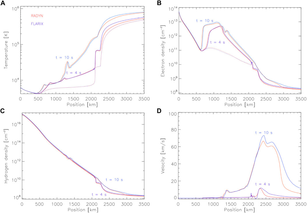
FIGURE 1. A comparison between RADYN and FLARIX, in which each code was purposefully stripped down to include as similar physics as possible. Despite very different numerical schemes, both codes produced strikingly similar results following injection of an electron beam. In each panel red is RADYN, blue is FLARIX, and the dotted lines are t = 0 s. Two snapshots during the flare are shown, at t = 4 s and t = 10 s. Panel (A) is temperature (B) is electron density (C) is hydrogen density, and (D) is velocity (upflows are positive). Figure adapted from Kašparová et al. (2019).
RADYN (Carlsson and Stein, 1992; Carlsson and Stein, 1997; Carlsson and Stein, 2002; Abbett and Hawley, 1999; Allred et al., 2005; Allred et al., 2015) is a radiation hydrodynamic (RHD) code (written in Fortran) that solves the coupled non-linear equations of hydrodynamics, charge conservation, time-dependent (non-equilibrium) atomic level populations, and radiation transfer on a 1D field-aligned adaptive grid (Dorfi and Drury, 1987). This adaptive scheme allows RADYN to resolve the strong shocks and gradients that usually form in flare simulations, and typically has 191 or 300 grid points (though this changeable). A semi-circular loop geometry is assumed, with one-half of a symmetric flux tube modelled, and a reflecting boundary condition at the loop apex designed to mimic incoming disturbances from the other half of the loop. This loop spans the sub-photosphere, through the chromosphere, transition region, and corona. Equations are solved in the linearised form using a fully implicit scheme (Abbett, 1998).
Species important for chromospheric energy balance are computed in detail, solving the NLTE radiation transfer and atomic level populations with the methods of Scharmer (1981) and Scharmer and Carlsson (1985). Those species are a six-level-with-continuum H i atom, a six-level-with-continuum Ca ii ion, and a nine-level-with-continuum helium atom/ion (with transitions of He i and He ii). In some models a Mg ii ion is also included. See Allred et al. (2015) for a list of the typical bound-bound and bound-free transitions. Bound-bound transitions are computed assuming complete frequency redistribution (CRD)1. To avoid overestimating radiative losses from the line wings, the Lyman lines mimic partial frequency redistribution (PRD) by either truncating at 10 Doppler widths, or modelling the line as a pure Doppler profile, depending on which version of the code is being used. Other species are included as a source of background continuum opacity via the Uppsala opacity package (Gustafsson, 1973). Optically thin losses are included by summing transitions from the CHIANTI atomic database (Dere et al., 1997; Del Zanna et al., 2015), excluding those transitions solved in detail. Downward directed incident radiation is included in the solution of the radiation transfer equation, so that photoionisations from X-ray, EUV and UV radiation are considered. This is achieved by calculating the sum of emissivities from transitions in CHIANTI, using the local temperature and density within each grid cell. Thermal conduction is a modified form of Spitzer conductivity, that saturates at the free-streaming limit, though, Allred et al. (2022) added the option to suppress thermal conduction using the method of Emslie and Bian (2018), which accounts for turbulence or non-local effects.
Flares are typically simulated by injecting a beam of non-thermal electrons at the apex of the loop, which are then thermalised, heating the plasma. Pre-2015 this was achieved using the analytic expressions of Emslie (1978) and Hawley and Fisher (1994), but post (Allred et al., 2015) this is achieved using Fokker-Planck kinetic theory, following McTiernan and Petrosian (1990), that better captures scattering terms, and which is applicable no-matter the target temperature (that is, there is no need to make a cold or warm target assumption, both are modelled using the actual target temperature). More recently still, Allred et al. (2020) developed the standalone open-source FP2 code to more accurately solve the non-thermal particle transport and energy dissipation, including the ability to include beam-neutralising return current effects, and to model the transport of non-thermal protons. FP has now been merged with RADYN. In all cases, non-thermal collisional ionisations and excitations of hydrogen by the particle beams are included, using the (Fang et al., 1993) approach, and post-(Allred et al., 2015), non-thermal ionisation of helium is included via data from Arnaud and Rothenflug (1985). Other options allow RADYN to model flare energy transport by mono-chromatic Alfvénic waves (Kerr et al., 2016) or by ad hoc time-dependent heating.
RADYN also allows us to calculate a posteriori (i.e., with no feedback on the plasma equations of mass, momentum, and energy) the time-dependent (non-equilibrium) populations and radiation transport of a desired ion via the minority species version of that code, MS_RADYN (Judge et al., 2003; Kerr et al., 2019b; 2019c). In this manner the hydrodynamic variables at each internal RADYN timestep, written separately from the main output file (that may have too low a cadence), can be used to calculate any additional species including non-equilibrium effects.
The HYDrodynamics and RADiation (HYDRAD) code was originally developed to model the field-aligned plasma physics of solar coronal loops subject to impulsive thermal heating (Bradshaw and Mason, 2003a; 2003b). Particularly careful attention is paid to the time-dependent (non-equilibrium) evolution of any desired ion species and their radiative coupling to the plasma, and to dynamically capturing the small spatial scales that arise in the solar transition region.
HYDRAD solves the conservative form (mass, momentum, and energy density) of the hydrodynamic equations for a two-fluid plasma, on a grid that employs adaptive mesh refinement of arbritrary order. The loops can have any geometry, length, inclination, or cross-section, and span footpoint-to-footpoint (for flare runs, to date), or as an open field line configuration (e.g., Scott et al., 2022), with a corona, transition region, and stratified chromosphere. Prior to (Reep et al., 2019) the chromospheric ionisation fraction was calculated with LTE assumptions, but Reep et al. (2019) implemented an approach that aims to capture NTLE hydrogen effects by approximating the radiation field without solving the full radiation transfer problem. Radiative losses in the chromosphere make use of the lookup tables of Carlsson and Leenaarts (2012), which account for losses from hydrogen, calcium and magnesium. Coronal radiative losses are calculated by summing the emissivity of all transitions within the CHIANTI database, as a function of the ion population fraction, where the ionization state can be given in equilibrium or calculated out-of-equilibrium, and the emission measure in each grid cell.
Flares are simulated by injecting a power-law distribution of non-thermal electrons at the loop apex, following the analytic treatment of Emslie (1978) and Hawley and Fisher (1994), with a sharp low-energy cutoff. This was implemented in Reep et al. (2013), and non-thermal collisional ionisation and excitations of hydrogen were added in Reep et al. (2019) using the (Fang et al., 1993) expressions for those rates. Flares driven by mono-chromatic (i.e., a single frequency) Alfvénic waves have also be modelled (Reep and Russell, 2016; Reep et al., 2018b).
Over the years HYDRAD has evolved into a flexible and powerful code capable of modeling a broad variety of phenomena including: multi-species plasma confined to full-length, magnetic flux tubes of arbitrary geometrical and cross-section variation in the field-aligned direction (Bradshaw and Viall, 2016); solar flares driven by non-thermal electrons and mono-chromatic Alfvénic waves, and the non-equilibrium response of the chromosphere; coronal rain formed by condensations in thermal non-equilibrium where the adaptive grid is required to fully resolve and track multiple steep transition regions (Johnston et al., 2019); and ultracold, strongly coupled laboratory plasmas, composed of weakly-ionized strontium (McQuillen et al., 2013; 2015).
HYDRAD is written in C++ and is designed to be modular in its structure, such that new capabilities (e.g., physical processes) can be added in a relatively straightforward way and handled robustly by the numerical scheme. It is also intended to be fairly undemanding of computational resources, though its needs do depend strongly on the particular nature of each model run (e.g., physics requirements, spatial resolution). The recently implemented NLTE solver for a 6-level hydrogen atom in the optically-thick chromosphere necessitated parallelization of part of the code (the OpenMP standard is employed) to recover acceptable runtimes. A significant performance gain may also be obtained when solving for the time-dependent ionization state of a large number of elements coupled to the electron energy equation via the radiative loss term. Otherwise, if this functionality is not required, then HYDRAD is generally most efficiently executed in single-processor mode with multiple instances running in an “embarrassingly-parallel” exploration of a parameter space, for example.
The code has been extensively deployed, tested, and used for a large number of scientific investigations on Windows PC, Mac, and Linux platforms, and found to be stable and robust. HYDRAD can be freely downloaded from its GitHub repository3.
FLARIX is a hybrid radiation hydrodynamic code (written in Fortran), comprised of three parts (Heinzel et al., 2016). Each component can be run as standalone codes, but are fully integrated within FLARIX. They are 1) a test-particle code that models the transport and thermalisation of non-thermal particles (Varady et al., 2010; 2014), 2) a 1D field-aligned hydrodynamic code (e.g., Kašparová et al., 2009), and 3) a time-dependent (non-equilibrium) NLTE radiative transfer code (MALI; e.g., Heinzel, 1995; Kašparová et al., 2003). FLARIX solves the hydrodynamics and NLTE radiation transport equations separately, but with feedback between the two codes so that, like RADYN, radiative heating and cooling from chromospheric lines and continua are considered, as is an accurate time-dependent NLTE hydrogen ionisation fraction.
FLARIX solves the single fluid hydrodynamic equations along one leg of a symmetric magnetic loop, that is assumed to be semi-circular. When solving those equations the time-dependent hydrogen ionisation fraction is obtained from the NLTE radiation transport code MALI, with the coronal segment assumed to be fully ionised (the ionisation fraction explicitly set to 1). The conductive heat flux is the Spitzer classical formula, and mechanical heating is applied to assure stability of the pre-flare atmosphere, which is typically a VAL-C (Vernazza et al., 1981) type stratification. This atmosphere spans the sub-photosphere through corona, with a fixed grid of
Flares are simulated by injecting a distribution of non-thermal electrons or protons, which are propagated and thermalised by Coulomb collisions (subsequently heating the plasma) using test particle and Monte Carlo methods, following the approach of Bai (1982) and Karlicky and Henoux (1992). This includes the relevant scattering terms, and pitch angle effects, and is equivalent to solving directly the Fokker-Planck equations (MacKinnon and Craig, 1991), but also provides a flexible means to investigate many aspects of non-thermal electron or proton interactions, such as magnetic mirroring and return current effects (e.g., Varady et al., 2014). Alternatively, the analytic expressions of Emslie (1978) and Hawley and Fisher (1994) can also be used. Non-thermal rates follow the (Fang et al., 1993) approach. For full details see: Kašparová et al. (2009), Varady et al. (2010), and Heinzel et al. (2016).
Note that for the code-to-code comparison of Kašparová et al. (2019), shown in Figure 1, RADYN and FLARIX were made as similar as possible as concerns the physics included (e.g., the atoms treated in detail, the optically thick loss functions, the form of electron beam heating).
Longcope and collaborators have developed a flare loop model which incorporates reconnection energy release by using thin flux tube (TFT; Spruit, 1981; Linton and Longcope, 2006) MHD equations. The axis of a thin flux tube evolves under a version of the ideal MHD equations expanded in small radius (Guidoni and Longcope, 2010). The tube is assumed to lay entirely within an equilibrium current sheet separating layers of magnetic flux with equal field strength but differing in direction by a shear angle Δθ. The magnetic pressure from the external layers maintains the field strength of the tube, but otherwise exerts no force on the tube’s axis. The tube evolves without reconnection under its own magnetic tension, and field-aligned pressure and viscosity. Energy transport is assumed to occur through thermal conduction, limited to the level of free-streaming electrons. The tube is initialized at the instant after a localized reconnection process within the current sheet has linked sections of equilibrium tubes from opposite sides of the current sheet. No further reconnection occurs, and any heating from the initializing event is neglected. In its subsequent evolution, the tube retracts under magnetic tension releasing magnetic energy and converting it to bulk kinetic energy in flows which include a component parallel to the tube. The collision between the parallel components generates a pair of propagating slow magnetosonic shocks, which resemble gas dynamic shocks as they must in the parallel limit. Absent thermal conduction, this evolution matches the classic models of Petschek reconnection including a guide field (i.e., component reconnection Longcope et al., 2009; Guidoni and Longcope, 2011; Longcope and Klimchuk, 2015). Solutions of the TFT equations show that thermal conduction carries heat away from the shocks, drastically altering the temperature and density of the post-flare plasma (Longcope and Guidoni, 2011; Longcope and Klimchuk, 2015; Longcope et al., 2016).
Guidoni and Longcope (2010) reported the first numerical implementation of the coronal TFT equations in a code called DEFT (Dynamical Evolution of a Flux Tube). A later implementation, called PREFT (Post-Reconnection Evolution of a Flux Tube; written in IDL), included optically thin radiative losses and a simplified chromosphere at each end of the reconnected flux tube, capable of reproducing chromospheric evaporation (Longcope and Klimchuk, 2015). Both versions have been adapted to include current sheets terminating in Y-points (Guidoni and Longcope, 2011; Unverferth and Longcope, 2020), although simulations are often done with a simpler uniform current sheet. Interactions with the current sheet plasma in the form of an aerodynamic drag force was later added (Unverferth and Longcope, 2021), and recent experiments impeded this drag force to investigate the role of MHD turbulence in prolonging heating into the flare gradual phase (Dr. William Ashfield, private communication, 2022). The chromosphere in PREFT is typically set to be isothermal (T ∼ 10 kK) and gravitationally stratified according to some density scale height.
Armed with the flaring atmospheres from the dynamic loop models we must then synthesise the emission that we predict IRIS would observe. This is true even in the case of RADYN and FLARIX where the radiation transfer of certain species is solved alongside the hydrodynamics, since the spectral lines observed by IRIS are not typically included in those solutions. This generally happens in one of two ways: 1) via an optically thin “coronal” assumption, using data from an atomic database such as CHIANTI alongside instantaneous properties of the flare atmospheres (e.g., emission measures, temperatures, and velocities); 2) via detailed NLTE radiation transfer calculations using snapshots from the dynamic simulations as input to post-processing code. Within the context of IRIS, the former is typically done for the Fe xxi, Si iv, and other optically thin transition region lines, and the latter for Mg ii, C ii, and other optically thick transitions or lines such as O i 1355.6 Å for which certain processes such as charge exchange require a radiation transport approach. Each approach has drawbacks and advantages.
In the optically thin line synthesis scenario the usual approach is to generate the contribution functions G (ne, T) (via a resource such as CHIANTI) that encapsulate the atomic physics processes that lead to the population and subsequent de-excitation of the transition in question. Normally this assumes ionisation equilibrium so that they peak at the equilibrium formation temperature of the ion in question. This may or not be a valid assumption in some scenarios. Codes like HYDRAD that track the non-equilibrium ionisation of minority species can instead use more realistic ionisation stratification. From these functions the emissivity in each grid cell can be calculated using the local plasma conditions within that cell:
where Ab is the abundance of the species, ne(z) is the electron density at height z, and nH, is the hydrogen density. The intensity in each grid cell is then Iλ,z = jλ,zδz, for a grid cell width δz. Once the intensity is known the spectral lines can then broadened by the instrumental profile, by the Gaussian thermal width, and by any assumed non-thermal width (e.g., due to microturbulence). Non-thermal broadening is the catch all term for any width in excess of the quadrature sum of the thermal and instrumental widths, the source of which is an active area of study. This could be due to local turbulence, unresolved flows, or something more exotic. When modelling it is usually not included without some apriori information (or guess!) about what it should be. Often some scheme is used to sum the intensity in each cell through height to provide the total emergent intensity. For example, this can be as basic as integrating through the full loop, or we can isolate certain locations such as the footpoints to integrate over. Other techniques attempt to take into account instrument properties, for example we can assume a semi-circular loop at disk center, orientated perpendicular to the Sun’s surface, and project each loop position onto an artificial pixel of some size inspired by the instrument we are trying to compare to (e.g., Bradshaw and Klimchuk, 2011, which is the norm for HYDRAD simulations).
When modelling optically thick lines by inputting snapshots from the flare simulations to radiation transport codes then it is usually the case that more advanced physics can be included in the solution that present in the original simulations, but at the expense of the dynamics. That is, non-equilbrium effects are often neglected and the statistical equilibrium population equations are solved instead. This can be mitigated somewhat by using in each atmospheric snapshot the electron density computed from a non-equilibrium solution, and in fact Kerr et al. (2019b) demonstrated using the minority species version of RADYN (MS_RADYN) that non-equilibrium effects can be, mostly, safely neglected when considering Mg ii even in flares (as was previously shown to be the case in the quiet Sun Leenaarts et al., 2013). In that instance, the inclusion of more advanced physics afforded by codes such as RH15D (Uitenbroek, 2001; Pereira and Uitenbroek, 2015), namely partial frequency redistribution (PRD), affected the line synthesis a great deal more than non-equilibrium effects. Post-processing flare snapshots through radiation transport codes typically involves providing the atmospheric stratification (e.g., height/column mass scale, temperature, electron density, velocity, microturbulence, H level populations or mass density) and a series of model atoms to solve (which in some cases form the basis of the non-hydrogen background opacities). The model atoms contain data about the atomic levels, the various transitions (oscillator strengths, damping terms etc.), thermal collisional excitation and ionisation rates, charge exchange rates, and the like. Thus, careful construction of the model atom is required to obtain a good result, including using the appropriate number of levels. There are three commonly used radiation transfer codes when processing flare atmospheres: RH, RH15D, and MALI. Of those, RH and RH15D are probably the most commonly used, and are in fact very similar to each other, the latter being a parallelised version of the former, allowing multiple snapshots to solved simultaneously. This greatly speeds up the problem as each 1D snapshot can take up to some tens of minutes or longer to solve if a very large number of transitions are desired, especially if PRD is being used.
Of the optically thick IRIS lines modelled in detail in flares, Mg ii is the most common, likely because it offers exceptional (though still largely untapped) diagnostic potential. Kerr et al. (2019a) and Kerr et al. (2019b) explored the impact of various radiation transfer effects when considering Mg ii in flares, partly in an attempt to determine if the large densities in flares meant that PRD could be neglected and the more computationally friendly complete frequency redistribution approach employed. Unfortunately it was the case that PRD was indeed required even in flares, but the hybrid angle averaged PRD approach of Leenaarts et al. (2012) was found to adequately approximate the full angle-dependent PRD solution and save an order of magnitude in computational time. Further, Kerr et al. (2019a) demonstrated that using a model atom with too few levels (e.g., 3-level-plus-continuum) produced different results than a larger model atom, in part due to the lack of cascades through upper levels present in larger model atoms (e.g., the 10-level-plus-continuum atom of Leenaarts et al., 2013). Aside from hydrogen, including other species in NLTE was found to not be required. A similar trade study has not yet been performed for other IRIS transitions in flares, though would be a worthwhile exercise.
Note that a new radiation transfer code capable of including time-dependent effects (if sufficiently high-cadence snapshots are available) and processes such as PRD and overlapping transitions has recently been developed: Lightweaver (Osborne and Milić, 2021). This exciting new resource has not yet been used to study IRIS observables (to my knowledge!) but should be employed in future efforts.
A major consequence of solar flare energy deposition is the driving of strong mass flows, which appear in spectral observations as Doppler shifted features either in the line core or as asymmetries in line wings. Both in early observations and modelling of flares (e.g., Fisher et al., 1985c; Fisher et al., 1985b; Fisher et al., 1985a; Fisher, 1989) a distinction was made between chromospheric evaporations that proceeded in a more “gentle” fashion and those that were “explosive”. Gentle evaporation is subsonic, whereas explosive evaporation is supersonic, reaching 100s km s−1, and is very impulsive in character, with a rapid rise to peak velocity. The overpressure and momentum balance from the explosive upflow scenario also produces downflows with speeds on the order a few × 10 km s−1 (chromospheric condensations) that are denser and propagate deeper into the chromosphere, appearing as redshifts in spectral lines. The Fisher studies determined that the energy flux delivered to the chromosphere and transition region was the deciding factor, with F = 1 × 10 erg s−1 cm−2 required to drive an explosive response. Those models used a fixed heating duration of t = 5 s, and a fixed Ec = 20 keV low-energy cutoff for the electron beam, and we know also that the low-energy cutoff can also an important parameter in determining the character of upflows/downflows (e.g., Reep et al., 2015). Note also that electron beams are not the only means to drive explosive chromospheric evaporation, and that they can be driven by a strong heat flux, for example.
As mentioned above, these upflows are produced by pressure gradients following flare heating, with momentum balance driving downflows. It is worth pointing out that the “dividing line” between upflows and downflows has been observationally identified in temperature space using Hinode/EIS data (e.g., Milligan and Dennis, 2009). In the footpoint of a C class flare, ions forming T > ∼ 1.5 MK exhibited large blueshifts whereas T < ∼ 1.5 MK exhibited redshifts (assuming ionisation equilibrium for their formation temperatures). Studying an X-class flare in which EIS observed several footpoint sources (Sellers et al., 2022) found similar results but with a range of flow reversal temperatures TFR ∼ [1.35–1.82] MK. This flow reversal point is located within the flare transition region, and roughly identifies the location of a pressure imbalance, and therefore heating location. It is an important benchmark for models to meet, though only one study to my knowledge has used this to test the physical processes in models. Allred et al. (2022) modelled the flare observed by Milligan and Dennis (2009) using RADYN, where they explored the effects of turbulent and non-local suppression of thermal conduction. Comparing the synthetic EIS profiles they found that suppression factors between 0.3 and 0.5 times that of the Spitzer values were most consistent with the observed flow reversal temperature, the magnitudes of upflows as function of temperature, and the non-thermal widths [studied for the same flare by Milligan (2011)]. In their study Allred et al. (2022) included the turbulent mean free path in the line synthesis, acting as a source of non-thermal broadening. Sellers et al. (2022) performed a very detailed observational study of the flows from many lines as observed by EIS and IRIS, as well as analysing the hard X-ray observations from RHESSI. Modelling those various flare footpoints, driven by non-thermal electron distributions inferred from the RHESSI observations as a function of time [for example using the RADYN_Arcade framework of Kerr et al. (2020), see below] would be a worthwhile endeavour to explore the pattern of upflows versus downflows. The upcoming Solar-C/EUV High-Throughput Spectroscopic Telescope [EUVST; Shimizu et al., 2019] will provide capabilities comparable to IRIS but with a significantly broader temperature coverage, which should also be a valuable resource for such studies.
I will not review the wealth of observational evidence and analysis of chromospheric evaporations and condensations here but refer the reader to recent reviews of EUV (Milligan, 2015) and UV flare spectroscopy (De Pontieu et al., 2021), and reference therein. Instead, in this section I highlight a few studies in which loop models of flares driven by typical non-thermal electron distributions were used to interpret signatures of mass motions in IRIS spectra, and in which IRIS spectra challenge the models.
The high spatiotemporal resolution afforded by IRIS has led to a plethora of studies of the chromospheric evaporation and condensation processes in flares. An important spectral line that has been used extensively for studying hot flare plasma is Fe xxi 1,354.1 Å, forming at around T ∼ 11 MK (in equilibrium conditions). This line exhibits large Doppler motions both in flare ribbon footpoints, and along the legs of flare loops, in excess of vDopp = 100 km s−1 and up to vDopp ∼ 250–300 km s−1 (e.g., Tian et al., 2014; Tian et al., 2015; Young et al., 2015; Graham and Cauzzi, 2015; Polito et al., 2015; Sadykov et al., 2015; Polito et al., 2016). At the same time the lines are initially extremely broadened, narrowing as the line returns to rest. Importantly, this line is entirely blueshifted within an IRIS spatial pixel (e.g., Young et al., 2015). That is, it does not just have a blue wing asymmetry alongside a stationary component, as was generally the case with MK lines observed during flares with lower-resolution observatories, the implication being that IRIS is resolving the flare footpoint source (if the filling factor is
To set these data in context I include a brief aside to discuss pre-IRIS observations of spectral lines produced in plasmas with a temperature in excess of several MK, though encourage the reader to see Milligan. (2015) for a fuller discussion. Blueshifts of up to a few hundred km s−1 from lines at
A superposed epoch analysis of IRIS Fe xxi 1,354.1 Å Doppler motions during an X class flare revealed a remarkably uniform behaviour within each footpoint (Graham and Cauzzi, 2015). Along the flare ribbon each footpoint initially showed Fe xxi vDopp ∼ 250 km s−1, with very little scatter, followed by a smooth decay in time back towards rest. Again with very little scatter, it took around 10 min for each source to return to rest (similar timescales have been seen in other flares). For various reasons (e.g., ribbon propagation timescales, rise times of UV or optical emission, duration of hard X-ray spikes) it is generally assumed that energy injection into each footpoint is more on the order of seconds to tens of seconds. In models that use those timescales the atmospheres undergo rapid global cooling, from flare temperatures towards quiescent temperatures, following cessation of energy injection and flows are quenched due to the collapse in chromospheric/transition region overpressure that drives the upflow of material. What then sustains these long lived upflows?
Similarly, in a number of flares the transition region Si iv resonance lines have been observed to exhibit redshifts lasting many minutes, in contrast to relatively shortlived chromospheric redshifts. Lifetimes of Si iv redshifts range from a few tens of seconds, to minutes, or even tens of minutes, seen in both high and low cadence observations (e.g., Brosius and Daw, 2015; Sadykov et al., 2015; Warren et al., 2016; Zhang et al., 2016; Li et al., 2015; 2017; 2019; Yu et al., 2020; Li et al., 2022; Ashfield et al., 2022). Pervasive net-redshifts, from
In this section I discuss some attempts to address the long duration upflows and downflows identified in IRIS observations with loop modelling, that focussed on the Fe xxi and Si iv lines.
In an effort to facilitate a more realistic model-data comparison of optically thin flare emission, Kerr et al. (2020) produced a synthetic flare arcade model that used an observed active region magnetic skeleton and RADYN field-aligned models. This model takes into account the superposition of loops and geometric effects (e.g., loop inclination, viewing angles) so that line-of-sight effects in the synthetic optically thin images and spectra are accounted for. A RADYN model was grafted onto magnetic loops extrapolated from a non-flaring active region (Allred et al., 2018), and were set off in sequence to mimic ribbon propagation (5 loops every 3 s). Within each voxel of the 3D space the differential emission measures (DEM; a measure of how much material is present within a temperature bin) and Fe xxi 1,354.1 Å spectra were synthesised, and, from the former, observables from the Solar Dynamics Observatory’s Atmospheric Imaging Assembly (SDO/AIA; Lemen et al., 2012) were synthesised. These were projected onto a 2D observational plane, with multiple voxels projected into a single pixel, so that superposition along the line-of-sight was included. This flare arcade model reproduced many aspects of Fe xxi Doppler shifts such as the magnitude of the blueshifts, the narrowing as they approached rest, and the localisation of the blueshifts to hot footpoints and lower legs of the loops. Figure 2 shows some synthetic Fe xxi spectra and a map of the arcade in this model. However, this model significantly underpredicted the decay time. Constructing a superposed Doppler flow similar to Graham and Cauzzi. (2015) showed only a t ∼ 50 s decay time of footpoint Doppler shifts, more than an order of magnitude too fast. Each loop in the arcade was from the same RADYN simulation, with t ∼ 25 s injection time, but the projected velocity differed depending on the loop geometry. Figure 3 illustrates the differences in decay time between the observations of Graham and Cauzzi. (2015) and the flare modelling.
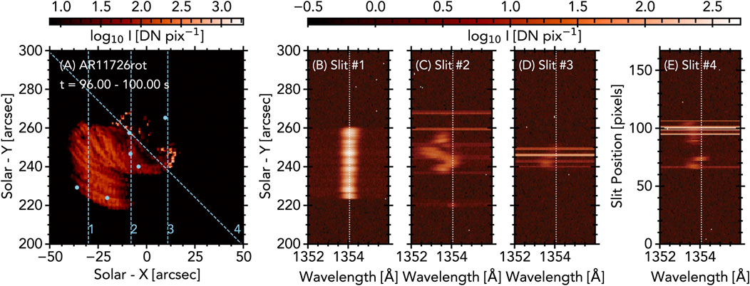
FIGURE 2. An example of RADYN_Arcade modelling of Fe xxi 1,354.1 Å, from Kerr et al. (2020). Panel (A) shows a map of the emission integrated over the Fe xxi line, with bright newly activated footpoints, and dense loops. Dashed lines are artificial slits, along which the spectra are shown in panels (B–E), where Doppler shifts and broadening is present. Bright horizontal strips are intense continuum enhancements at loop footpoints. © AAS. Reproduced with permission.
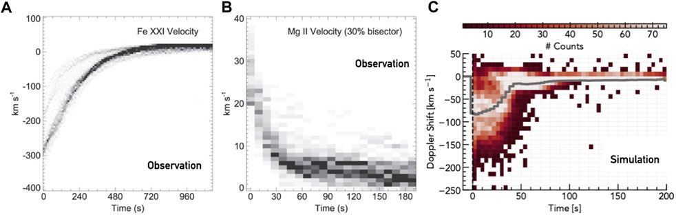
FIGURE 3. Comparing an observed superposed analysis of mass flows to the modelled upflows. Panel (A) shows the Fe xxi 1,354.1 Å Doppler shifts obtained from fitting Gaussians to IRIS observations of the 2014-September-10th X-class flare, and panel (B) shows the Mg ii subordinate line Doppler shifts from that same flare, obtained via a bisector analysis (negative velocities are blueshifts, positive are redshifts). Both are adapted from Graham and Cauzzi. (2015). Panel (C) shows the synthetic Fe xxi 1,354.1 Å line Doppler shifts from the RADYN_Arcade model of Kerr et al. (2020), where the grey line represents the mean. Clearly the modelled upflows subside an order of magnitude too quickly. © AAS. Reproduced with permission.
This result was perhaps not unexpected. It is generally the case that flows subside not long after the cessation of energy injection, which alongside rapid global cooling removes the pressure imbalance in the absence of heating, quashing the upflows. Reep et al. (2018a) contains some detailed examples of this, where upflows in either a single model with bursty injection, or a multi-threaded model with simultaneous individual heating events, disappeared shortly after the electron beams were switched off. As well as unexplained lengthy upflows we have a mix of short and long duration condensations as discussed above, which are also frustratingly hard to explain. The Fisher (1989) models of condensations predict that the downflows last t ∼ 30–60 s, almost regardless of particle injection timescales. Once the chromosphere has been shocked out of equilibrium, the condensation propagates deeper, but accrues mass as it does so, and decelerates. Even if energy release is continuous over an extended time it seems hard to drive longer lived downflows as the chromosphere reaches a new equilibrium and is no longer shocked. The chromospheric timescales predicted by models are not as incongruous with observations as the upflows into the corona. Doppler shifts observed in Mg ii and other chromsopheric lines have lifetimes not too dissimilar from the modelled 30–60 s (e.g., Graham and Cauzzi, 2015; Graham et al., 2020), shown in the middle panel of Figure 3.
One means to obtain long duration upflows of Fe xxi 1,354.1 Å is simply to bombard the atmosphere with an electron beam for an extended period of time. To reproduce the
An alternative means to achieve long duration upflows, and to address similarly long lived transition region downflows is multi-threaded modelling in which each IRIS pixel is assumed to be comprised of many strands embedded within that volume, with one loop model representing just one of these strands. Warren et al. (2016) studied a B2 class flare, noting that whereas Mg ii exhibited discrete bursts of intensity enhancements with associated redshifts, the Si iv and C ii resonance line redshifts were more systematic, not returning to rest for many minutes. Their lightcurves were also sustained but showed more structure, with a few strong spikes. To explain these transition region observations (Reep et al. 2016) used HYDRAD loop models in a novel way. They ran 37 electron beam driven simulations, with the spectral index and low-energy cutoff inferred from RHESSI observations, and a range of energy fluxes spanning F = 108–11 erg s−1 cm−2, applied for t = 10 s to each loop. From each loop, the Si iv spectra were synthesised, applying Doppler shifts as appropriate. They then randomly sample emission from N threads, activating randomly with an average rate of one per r unit time, and with a power law in energy flux space guided by the FUV intensity distribution from observations of Warren et al. (2016), dividing the total summed intensity by N. N and r are connected by the requirement that N × r > τ, for τ some observed duration, for example the duration of redshifts. Within each individual strand, weak energy deposition (
Through trial and error to ensure smooth and longlived Si iv Doppler shift lightcurves, (Reep et al., 2016) determined that to reproduce the (Warren et al., 2016) observations, N ≥ 60 threads were need per IRIS pixel, activating with a rate r ≤ 10 s, and with a minimum flux of F = 3 × 10⁹ erg s−1 cm−2. Burstier lightcurves resulted from decreasing the activation rate (increasing r), or allowing a smaller minimum energy so that large excursions resulting from the strongest threads were more prominent (recall that some observations of larger flares showed quite bursty Si iv Doppler motions). Comparing the observed and modelled slopes of the emission measure distributions (EMD) can help further constrain N and r. A smaller r forces a higher N, the consequence of which means there are many more cooling loops at any time, boosting the low temperature end, and thus the slope, of the EMD at those temperatures.
Building upon this framework, Reep et al. (2018a) performed similar modelling that could simultaneously address the long lived Fe xxi upflows and Si iv downflows. They again kept δ = 5 and Ec = 15 keV of the non-thermal electron distribution fixed, but this time allowed the duration of energy injection onto each thread to vary. A triangular pulse with equal rise and fall times, with total durations ranging tdur = [1–1,000] s, in increments of 0.1 in log space was used, with peak energy fluxes ranging Fpeak = [108–1011] erg s−1 cm−2 (providing 341 simulations total). Both Si iv and Fe xxi emission was synthesised from each loop model under optically thin conditions. Comparing two of their single loop models, Reep et al. (2018a) first demonstrated that with longer energy deposition timescales, the upflows persist, but that downflows diminish even before the energy deposition ceases, confirming earlier results from Fisher’s models. Once the chromosphere has been shocked and produces a condensation, it is difficult to re-shock just with continuous energy deposition. Further, the weaker simulations did not produce sufficiently hot, sufficiently dense loops to emit strongly in Fe xxi (for intermediate energy fluxes non-equilibrium effects could lead to a delay in the formation Fe xxi). Comparisons of the peak densities, temperatures, and mass flows produced by the grid of individual loops demonstrated that in addition to the energy flux, and low-energy cutoff, the duration of energy deposition likely plays a role in determining if evaporation proceeds explosively or not.
Performing the multi-threaded modelling with various setups (variously fixing or changing values of N, r, Fmin, α, where α describes the slope of the energy flux distribution) using this HYDRAD grid, (Reep et al., 2018a) found the following general conclusions. Longer heating durations produce smoother lightcurves, as loops heated by shorter durations cool too fast. For a mix of heating durations, a median of tdur = [50–100] s does a better job of reproducing the combination of long lived up- and downflows. More sustained past heating tdur > ∼ 100 s results in the initial set of loops dominating the signal, but their downflows still subside after
Applying this model to estimate the number of strands per IRIS pixel in an observed flare, the M class event on 2015-March-12, (Reep et al. (2018a)) find they can largely reproduce aspects of the observations with r = [3, 5] s, and heating durations between tdur = [30–300] s. However, they note that the observed Si iv intensities decrease with time, possibly indicating that the maximum energy flux in the distribution of threads decreases over time. This comparison is shown in Figure 4, with the observations on the left, and the N = 200, r = 5 s multi-threaded HYDRAD model on the right. Comparing to Figure 3, the multi-threaded approach clearly does a better job at reproducing the extended Doppler shifts.
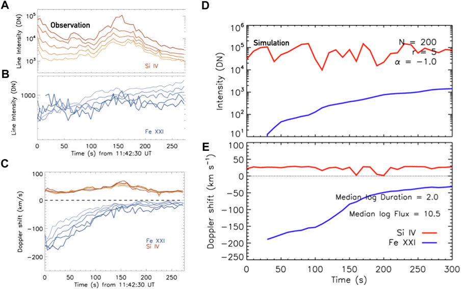
FIGURE 4. Explaining the observed long-duration flows with multi-threaded modelling. Panels (A–C) show observations of the M class 2015-March-12 solar flare, where from top to bottom we see the Si iv 1,403 Å intensity (yellow/brown colour scale), the Fe xxi 1,354.1 Å line intensities (blue colour scale), and the Doppler shift of each line (negative velocities are blueshifts, positive are redshift). The multiple lines shown for each quantity represent five different pixels in the flare ribbon. Panels (D,E) show the equivalent properties, but for a multi-threaded HYDRAD simulation, with N = 200 threads per IRIS pixel. In those panels red shows Si iv and blue shows Fe xxi. This model does a good job at capturing the duration of flows but does not exhibit the decrease in Si iv intensity towards the latter stage of the flare. Figure adapted from Reep et al. (2018a). © AAS. Reproduced with permission.
To tackle the chromospheric predictions in their multi-threaded modelling (Reep et al., 2019) synthesised O i 1355.6 Å and Mg ii k line spectra via RH15D with HYDRAD flare atmospheres as input, after first modifying the treatment of the chromosphere in HYDRAD. Before Reep et al. (2019) the H ion fraction, and therefore estimates of radiative losses from the (Carlsson and Leenaarts, 2012) lookup tables, in the HYDRAD chromospheres were based on an LTE treatment that used the local temperature and electron density, assuming collisional rates dominated. To improve this, and to obtain better estimates of H ionisation stratification, electron density stratification, and radiative losses, they turned to the approach of Leenaarts et al. (2007), who followed the work of Sollum (1999). In this model the radiative and collisional rates for each transition of H were considered in order to obtain level populations for five levels of H plus the proton density. The collisional rate data were taken from standard sources. Obtaining the radiative rates without calculating the radiation field by solving the full NLTE radiation transfer problem required estimating the radiation field stratification above some critical height (below which the atmosphere could be assumed to be LTE), varying as a function of column mass above this height. Ultimately, the brightness temperatures were obtained as a function of height, and used to calculate the radiative rates. Reep et al. (2019) follow the Sollum (1999) results, but make some important modifications to account for the fact that the radiation field at the top of the chromosphere differs in flares. They note the relation between electron density and line intensity, using this to vary the brightness temperature at the top of the atmosphere as a function of electron density, with a grid of RADYN models serving as a guide.
Armed with this new model chromosphere, the parameter space of Reep et al. (2016) was re-run to model the observations of Warren et al. (2016), and multi-threaded models of the chromospheric lines calculated via processing HYDRAD flare atmospheres through RH15D and combining the emission in the same manner as Reep et al. (2016). Reep et al. (2019) argue that the single loop model cannot explain the O i emission, since it is strongly redshifted in the model but largely stationary in the observations. It was also far too bright in the models. Various setups of the multi-threaded approach managed to produce O i Doppler motions consistent with Warren et al. (2016) observations, but the ratio of O i to C i was not consistent (O i was too bright). The Mg ii results were also consistent with the observations, showing bursty redshifts lasting throughout the heating phase. Something not addressed by Reep et al. (2019) is if we might really expect the chromospheric emission in a multi-threaded model to freely escape without radiation transfer effects between each closely space thread, which may confuse the picture of the very optically thick Mg ii lines in this model (though O i is very likely optically thin in flares). Single loop models likely suffer similar issues with 2D/3D radiation transfer, though often the assumption is that they are embedded in a ribbon-like structure that evolves similarly, rather than having many tens or hundreds random energisation events within the small volume of an IRIS pixel. A recent study using RADYN flare models and Lightweaver has demonstrated the importance of including 2D and 3D radiation transfer (Osborne and Fletcher, 2022), though focussing on quiet Sun nearby a ribbon. A similar model that explores the effects within the ribbons or footpoints themselves (i.e., an inhomogenous ribbon) would be very interesting and worthwhile!
The application of multi-threaded modelling to the problem of long lived flows has been largely successful, with important implications if true, for example that individual threads may be smaller than 1/100 arcseconds for N ∼ 60, scaling inversely with N. While this model alleviates the demand of continuous energy injection into a single thread for many minutes, it still demands the injection for many minutes into an area the size of a single IRIS pixel (i.e., a single localised volume), and for up to
An important facet of loop models that is typically ignored when modelling solar flares is area expansion along the loop. In most flare loop modelling the loop is assumed to be semi-circular with uniform cross-sectional area. However, given that the magnetic field decreases with height from photosphere to corona, in order to conserve magnetic flux, the area of the loops should presumably expand with height. This could also help alleviate the stark model-data discrepancies of transition region spectral line intensities (see the discussion in the detailed study of Reep et al., 2022a). Including area expansion in our models is relatively straightforward, but the questions are by how much should the area expand, where should this expansion begin, and does this have a strong effect?
The uncertainty here is not helped by the fact that it is observationally very tricky to identify the appropriate values to use. In fact, observations of both quiescent and flaring coronal loops do not seem to show significant expansion along their length, varying by only
In their continuous-expansion experiments, the expansion factors, from footpoint to loop apex, tested were Aexp = [1, 11, 43, 116]. Each factor was used in an electron-beam driven flare simulation, with a deposition duration of 100 s. The time taken to reach peak density was delayed with increasing area expansion, producing much longer cooling phases than typically seen in flare simulations. There is an extended period of time where the peak densities remain roughly constant and the temperatures decrease slowly via radiation, with draining only occurring after the temperature drops below T = 100 kK. Area expansion modified the T ∼ n2 relation so that the dynamics of the radiative cooling phase of the flares were very different than a loop with uniform cross-section. Upflows through the high temperature coronal loops persist well beyond the energy injection phase, in contrast to results discussed previously. Sound waves that result from sloshing of material during the flare gradual phase are also suppressed with increasing area expansion, and the magnitude of evaporative upflows reduced as the plasma encounters larger cross-sections. Sun-as-a-star irradiances synthesised from these models were reduced for loops with increasing area expansion but equal total volume, and the longer draining and cooling timescales results in sustained emission. Similar results were found for area expansion localised near the transition region, but with smaller changes to the timescales compared to the continuous-expansion case when the expansion occurs closer to the flare footpoint in the transition region. Sounds waves were also less suppressed in this scenario.
The assumption of a semi-circular loop was also interrogated, with a modification made to the gravitational acceleration term parallel to the loop to make the loops more elliptical. This has a seemingly minor effect, mostly on the draining timescales due to slightly weaker gravitational acceleration.
It is not yet known what the appropriate values of area expansion to use are, but Reep et al. (2022b) has convincingly demonstrated that this factor should not be ignored, particularly for the gradual phase of each footpoint. Indeed, this may negate the requirement for continuous energisation of many threads within a single IRIS pixel in order to maintain long-lived flows. Hopefully further exploration of these impacts will shed light on the appropriate values to use.
Redshifted, broadened, emission appearing in the wings of strong chromospheric lines has been observed for many decades, for example famously in Hα (e.g., Ichimoto and Kurokawa, 1984) who found short-lived (
IRIS has now observed many example of chromospheric downflows in flares, especially in the Mg ii NUV spectra, at sub-arcsecond resolution (e.g., Kerr et al., 2015; Liu et al., 2015; Graham and Cauzzi, 2015; Rubio da Costa et al., 2015; Kowalski et al., 2017; Panos et al., 2018; Huang et al., 2019; Graham et al., 2020). Kowalski et al. (2017) identified similar features in weaker, more narrow chromospheric lines observed by IRIS, where they could appear as distinct components that persisted only for the duration of one 75 s raster. Modelling of the two brightest footpoints in that flare, using RADYN, revealed that a rather high energy flux of non-thermal electrons was required to be injected into each footpoint, but that the dwell time on each footpoint could be different. A short pulse (Δt = 4 s) and a longer pulse (Δt = 8 s) were necessary to produce consistent ratios of Fe ii redshifted component intensity to line core intensity within each different footpoint. This bore similarities to the conclusions of Falchi and Mauas. (2002) who suspected that the red-asymmetry of certain line wings could originate from a condensation at a greater altitude than the usual line formation height.
Higher cadence (δt = 9.4 s) IRIS observations of the 2014-September-10th X-class flare revealed that in addition to spectra exhibiting redshifted cores and red-wing asymmetries in chromospheric species (Graham and Cauzzi, 2015), many spectra contained separate components with redshifts indicating downflows of the order 25–50 km s−1. These components were at times sufficiently far from the strong, mostly stationary, components that they were dubbed “satellite” components (Graham et al., 2020). These were most apparent in singly ionised and neutral transitions that produce spectral lines that were generally more narrow than the very strong resonance lines observed by IRIS. For example, they were seen in Mg ii 2,791.6 Å, Fe i 2,714.11 Å, Fe ii 2,813.3 Å, Fe ii 2,814.45 Å, C i 1,354.284 Å, and Si ii 1,348.55 Å. The lefthand side of Figure 5 shows examples of these satellite redshift components for the Fe ii 2,814.45 Å lines, where it can be seen that the satellite components were broader than the primary more intense “stationary” component, and were observed to migrate towards, and ultimately merge with, the primary component over a period of
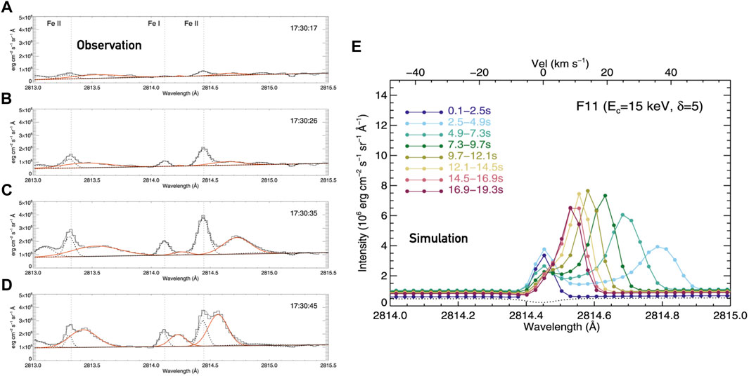
FIGURE 5. Modelling red wing asymmetries and satellite components. Panel (A–D) show a series of snapshots of the Fe ii 2,814.5 Å line, observed by IRIS in the 2014-Sept-10 flare, where a stationary and satellite component are clear. The black solid histogram lines are the data, the black dotted line is the Gaussian fit to the stationary component, the red line is the Gaussian fit to the satellite component, and the thin grey line is the sum of the two components. Panel (E) shows RADYN modelling of the Fe ii line from that flare, which was able to reproduce the satellite component, though with an overestimated intensity. Figure adapted from Graham et al. (2020). © AAS. Reproduced with permission.
Using Fermi/GBM (Meegan et al., 2009) hard X-ray data, Graham et al. (2020) performed data-driven modelling of the Fe ii 2,814.45 Å line from that flare. The spectral properties of the non-thermal electron distribution were obtained (δ = 5, Ec = 15 keV), along with the total instantaneous power carried as a function time, averaged over 10 s time bins to be consistent with the IRIS data. Crucially, the energy flux (power/area) was estimated by carefully measuring the newly brightened area of IRIS SJI images at each time, with the rationale being that this revealed the locations into which the non-thermal electrons observed in Sun-as-a-star Fermi data were being injected at any snapshot. Using different thresholdings to define this area provided a range of energy flux densities on the order 1011–12 erg s−1 cm−2. Finally, the duration of energy injection into each footpoint was estimated from the width of a half-Gaussian function fit to the rise time of the Fe ii spectra [similar to the approach of Qiu et al., 2012], revealing a dwell time5 of tinj ∼ 20 s. RADYN modelling was performed with these derived parameters as input, in which a prominent condensation rapidly formed, with downflowing speed of up to 50 km s−1, an electron density in excess of 1014 cm−3 and a width of only Δz = 30–40 km.
Modelling the Fe ii lines, including averaging the synthetic spectra over the IRIS τexp = 2.4 s exposure time, revealed that this condensation did indeed result in a satellite component forming, that subsequently decelerated towards the stationary component as the condensation pushed deeper. Synthetic satellite components are shown in the righthand side of Figure 5, where colour represents time in the simulation. Figure 6 shows the contribution function to the emergent intensity (i.e., where the line forms) of the Fe ii line. The bright contribution from redshifted material is obvious, as is the narrowness of the condensation appearing in the upper chromosphere. From the formation properties of the lines, such as Figure 6, we can understand the origin of the satellite components. Flare heating in the chromosphere enhances the lines, but in a region without meaningful mass flows so that the near-stationary component is bright. Once the condensation develops at the top of the chromosphere/base of transition region and becomes dense it begins to produce Doppler shifted emission from those same ions. Since the stationary components are relatively narrow the very redshifted emission appears as a separate line. As the condensation accrues mass while it propagates deeper, it slows, such that the Doppler shift of the satellite component reduces and it merges with the stationary component, taking on the red-wing asymmetry appearance. The optical thickness of the lines comes into play as those lines that are very optically thick and form higher in altitude (e.g., the Mg ii or C ii resonance lines) will more quickly see the merging of the stationary and redshifted components (with the whole line appearing redshifted in many cases). In those cases the large opacity means that little light can escape the top of the condensation once enough density is accrued, and so the stationary component is not visible. For lines with smaller opacity both components can be seen. Further, the large opacity broadening of the resonance lines means that the redshifted component would likely not appear as a fully separate component, rather as a red wing asymmetry.
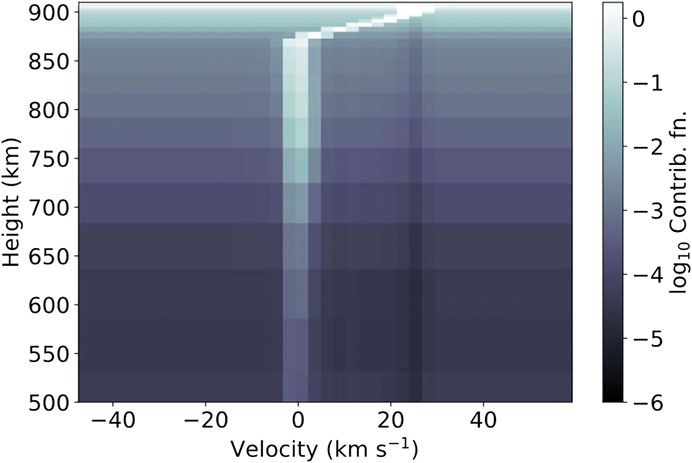
FIGURE 6. The contribution function to the emergent intensity of Fe ii 2,814.45 Å. Integrating through height yields the emergent intensity. Note the intense, but narrow, condensation in the upper chromosphere producing bright, redshifted satellite component alongside the stationary component. Figure from Graham et al. (2020). © Copyright AAS. Reproduced with permission.
The intensity of both the surrounding continuum and the stationary components agreed with the observations, as did the magnitude of the Doppler shifts. However, several discrepancies did exist. The satellite component was much too intense, outshining the stationary component, and was much too narrow (as discussed in Paper 2 Kerr submitted of this review line widths are a perennial problem). The onset and evolution of the satellite components also occurred on a more aggressive timescale compared to the observations, though not egregiously so (a factor 2–3× faster). Finally, varying the low-energy cutoff or energy flux illustrated how sensitive the properties and evolution of the condensation are. For example, increasing the energy flux to the upper range of the estimates in this particular case produced a condensation much too fast compared to the observations with a larger-than-observed continuum intensity. Similarly, increasing the low-energy cutoff meant that the condensation developed too late and was too slow. This demonstrates the possibility that such observations can be used to guide or constrain the range of plausible electron beam parameters consistent with the evolution of UV radiation in a particular flare (though I stress “guide”; I do not believe we are yet in a position to use them independent of X-ray observations).
Graham et al. (2020) explicitly demonstrated how useful high-cadence spectral characteristics are in confirming the inferred properties of the electron beam. They also demonstrated why we should pay attention to weaker lines in addition to the more commonly studied resonance lines. Similar condensations were shown in the models discussing the much broader Mg ii h and k lines (Kerr et al., 2016; Kerr et al., 2019a; Kerr et al., 2019b) but in those cases instead of producing satellite components, they produced small asymmetries in the red wings. In comparison to the resonance lines of Mg ii and C ii, Fe ii 2,814.45 Å has a much lower opacity, probing more easily the deeper layers of the chromosphere (Kowalski et al., 2017). Earlier modelling of condensation timescales found a similar discrepancy in the timescales compared to Hα observations (Fisher, 1989) as those noted by Graham et al. (2020). IRIS’s very high spatial resolution suggests that the answer to this discrepancy does not lie in the superposition of flows from many unresolved elements (though note that the difference in timing is only a factor 2 or so, not the order of magnitude that is the case for evaporative upflows!). An overdense condensation could explain why the modelled satellite components were brighter than the stationary components. Though not focussing on red wing asymmetries, Kerr et al., 2019a shows Mg ii 2,791 Å lines with a redshifted satellite component that is weaker than the stationary component. In that simulation the condensation is not very dense, hence the smaller intensity. A means to obtain an estimate of the electron density from the broadening of high-order Balmer lines was presented by Kowalski et al. (2022), and the effects of improved Stark broadening are now included in RADYN and RH. Coordinated DKIST and IRIS observations of the Balmer lines and FUV/NUV spectra would shed light on this discrepancy and condensation densities (see also the comprehensive discussion regarding model-data discrepancies in Kowalski et al. (2022), Section 5).
It is not yet known if the physics of flares scales from the very large (M and X class events) to the very small (micro or nanoflares), but it is a reasonable assumption that electrons could be accelerated even in small events (see recent evidence from NuSTAR observations of (sub-) microflares Glesener et al., 2020; Cooper et al., 2021). Rapid variations in Doppler motions (both blue- and redshifts) and intensities have been observed at the base of coronal loops in the transition region, leading (Testa et al., 2014 and Polito et al., 2018) to investigate via RADYN modelling if non-thermal electron distributions injected into the transition region from the corona could explain these “nanoflare” signatures. The total energy deposited was estimated as being 6 × 1024 erg (based on Parker, 1988), compared to 1030–32 erg for moderate-to-large flares. This equated to an energy flux of 1.2 × 10⁹ erg s−1 cm−2 considering the area of the footpoint emission, and an assumed dwell time of 10 s based on lifetimes of short-lived brightenings in transition region moss. Note that the total energy, and the energy flux, associated with the nanoflares observed by Testa et al. (2014) and Polito et al. (2018), while fairly small, is not so different from an individual flare loop; it is the much greater number of flare loops/greater flare volume that leads to the larger total energy.
Polito et al. (2018) performed a parameter study sampling different non-thermal electron distributions, and injected those electrons into two pre-flare atmospheres, one initially cool and tenuous (a low density corona at 1 MK), and one hotter and dense (a high density corona at 3 MK). The latter represents an active region loop, the former being more quiet Sun-like, and both had extended plateaus of higher temperatures in the chromosphere compared to VAL-C type atmospheres, maintained in the model by artificial non-radiative heating. The electron energy spectra had low energy cutoffs in the range Ec = [5, 10, 15] keV. The low-energy cutoff, Ec, had a strong impact on the subsequent dynamics. Flares with a small Ec efficiently heated the corona, driving the whole transition region to greater column mass, and therefore resulting in Si iv redshifts, along with explosive evaporation. The corona is very tenuous, so it is easy to drive fast flows even at these low energy fluxes if Ec is low such that energy is largely deposited in the upper transition region/lower corona. Larger values of Ec means that there are relatively more high energy electrons that thermalise somewhat deeper, so that gentle evaporation through the transition region occurred and upflows at the temperatures that form Si iv were present. Initially dense loops resulted in lower intensity emission and slower flows compared to initially tenuous loops. Loop length was also an important factor for the dense loops, with longer loops resulting in a larger portion of electrons thermalising in the corona.
The dynamics of the loops had a direct impact on the synthetic emission, allowing a straightforward comparison to observations. Polito et al. (2018) synthesised Si iv resonance line emission, degrading the spectra to IRIS resolution and count rates. Tenuous loops result in a very intense Si iv response for all simulations, but reaching a peak in the 10 keV experiment. For the dense loops, the softest non-thermal electron distribution (Ec = 5 keV) did not produce an appreciable response of Si iv on rapid timescales. Blueshifts were seen in simulations with Ec > 10 keV, whereas redshifts were seen in simulations with Ec = 5 keV, as illustrated in Figure 7 that shows the Si iv spectra and lightcurves for simulations with different values of Ec. Once the loops have filled following evaporation and become denser, electrons thermalise more easily in the corona where they cause further heating. Redshifts were also seen in experiments in which the same magnitude of energy was deposited directly in the corona and allowed to conduct through to the lower atmosphere. No blueshifts were seen in that scenario.
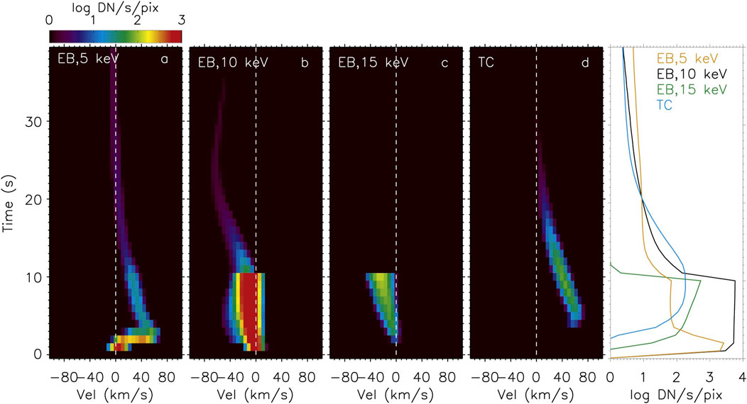
FIGURE 7. Demonstrating that non-thermal electron beams can produce blueshifted emission with Ec > 10 keV in nanoflare simulations using RADYN. Panels (A–C) show Si iv spectra for electron beams with different Ec, panel (D) shows the spectra in the case of a conduction driven flare, and the rightmost panel shows the lightcurves from each flare. Figure from Polito et al. (2018). © AAS. Reproduced with permission.
Polito et al. (2018) speculate that based on their loop modelling, the observations of impulsive brightenings in the transition region at the base of coronal loops are consistent with energy input to an initially cold, tenuous loop. Since observations show both blue and redshifted emission, this suggests that conduction driven heating of loop footpoints at the transition region alone is not consistent with the observations. That is, IRIS observations combined with RADYN modelling suggest that particles are accelerated even in small-scale brightenings, contributing to active region heating.
Since the development of condensations and evaporations during flares is closely tied to the properties of energy injection, there could exist correlations between these flows inferred from spectral lines. Sadykov et al. (2019) explored the potential of such correlations using IRIS data, and also via RADYN modelling of electron beam driven flares. Seven flares were selected that conformed to a strict set of criteria, including fast scans (
These same lines were modelled from a grid of electron beam driven flare simulations produced by the F-CHROMA consortium using RADYN7. This grid samples a large parameter space of non-thermal electron distributions, that were injected into a VAL3C-like (Vernazza et al., 1981) pre-flare atmosphere. Energy was injected for t = 20 s, in a triangular profile peaking at t = 10 s. While most of the F-CHROMA grid represents relatively weak-to-moderate heating events, it is a very useful resource for studying flare processes and I encourage the reader to access it for their own research.
Sadykov et al. (2019) selected 20 flares from this grid that loosely were consistent with the observationally derived non-thermal electron distribution properties. For the observational analysis of hard X-rays, the area selected to determine the energy flux into the chromosphere was the 50% contour of the hard X-ray source. As I discuss in other sections, this very likely is an overestimate of the areas, and thus an underestimate of the actual energy flux. At a cadence of 1 s, synthetic C ii and Fe xxi spectra were obtained from the RADYN atmospheres, using RH15D and data from CHIANTI, respectively. In the latter case, Fe xxi emission was summed through the full extent of the half-loop, so no geometric effects of extended emission regions were considered. The same Doppler shift metrics derived from the observations were then obtained from the models.
A statistical analysis revealed that there was no meaningful correlation between observed mean C ii redshifts and non-thermal energy flux, but there was in the models. While still not very statistically significant, the observed maximum redshifts did show a correlation with the injected non-thermal energy flux. Similarly, there were no meaningful correlations between observed Fe xxi blueshifts and non-thermal energy flux, but there were in the models. Further discrepancies existed also. Unlike the observations, the models predicted that in some cases there should be modest C ii blueshifts. Observed flows of Fe xxi were on the order 100 km s−1, consistent with the range of reported values in other studies, but some of the models exceeded 500 km s−1. The differences between the models and data suggest that either the flares being compared were not apples-to-apples (in the sense that the energy flux in the observed flares may have been underestimated due to the choice of using hard X-ray areas, and so larger than those used in the models), or that physics is missing from the models.
As an example of the latter, recent work by Allred et al. (2022) to include the suppression of thermal conduction in RADYN simulations due to turbulence and non-local effects revealed slower upflows, and a shift in the altitude at which the transition region forms. The latter results in the switch from upflow to downflow occurring at a different temperature for a given set of electron beam parameters [in this case, those observed by Milligan and Dennis (2009)]. That study focussed on EUV observations, but future work will include IRIS observables, which may address the discrepancies discovered by Sadykov et al. (2019).
In this first part of a two-part review of IRIS observations and flare loop modelling I have introduced the four main modern flare numerical models that have been used alongside IRIS data: RADYN, HYDRAD, FLARIX, and PREFT (though these latter two feature more in part two of this review). As well as this I have given an overview of how we synthesise IRIS observables from those models. With those models and the high spatial-, spectral-, and temporal resolution observations provided by IRIS we have learned much about flare-induced mass flows, that in the standard flare model assumed energy transport via directed beams of non-thermal electrons.
Though there are details to work out, recent modelling work performed in an attempt to explain long-lived mass flows induced in flare footpoints, at the scale of IRIS resolution elements (0.3–0.4″), has convincingly demonstrated that there is a seeming demand for continued energy deposition into each footpoint for up to several minutes. Multi-threaded modelling results also suggests that this energy deposition is not coherent; that is, not every thread is energised at the same time, different threads (of which there may be many hundreds within each 0.167″ pixel) are energised at different times, and for different durations. There are questions persisting here. We do not know if electrons are accelerated, and subsequently thermalised within the same small volume of an IRIS pixel for many minutes, nor even how long this would occur for on a single thread. Hard X-ray sources currently lack the high spatial resolution obtainable at UV wavelengths, and also have historically had low dynamic range so that only the strongest sources are observable. Still, hard X-ray sources are seen to move over time in a flare and not always linger for a long duration in a single location, and strong hard X-rays are not observed in the gradual phase.
IRIS observations of redshifted satellite components and red-wing asymmetries have been successfully modelled using field-aligned loop models in which non-thermal electron beams drive strong condensations. These condensations are narrow, and dense, producing redshifted emission that slows over time. Again, there are details to work out. For example the ratio of the redshifted to stationary component is not well-captured in models compared to observations. This could suggest an over-dense condensation in the model compared to the observation. The disparity between timescales of the redshifted components in the models compared to the observations is not as stark as those in the upflow scenario; condensation timescales in the models are more aggressive than in the observations, but do not reach the more than an order of magnitude differences that the modelled upflows suffer from.
Curiously, this means that we have different solutions to each problem: multi-threaded models with continued energy release is required to understand upflow behaviours, whereas single loop models with suitable non-thermal electron beam parameters that produce condensations can explain the chromospheric downflows. Transition region flows (e.g., Si iv) are somewhat of an in-between case, with some observations requiring multi-threaded observations, but individual bursts in other observations can be captured with single loop modelling (see also Paper 2 Kerr, submitted). It is important that we now work to reconcile this seeming contradiction between the need for multi-threaded versus single loop modelling for different parts of the atmosphere. One resolution may be to have continued energy deposition into the transition region and upper chromosphere but at a magnitude too weak to drive strong condensations. This was hinted at by the results of multi-threaded modelling which suggested that the intensity of Si iv emission should decrease towards the end of the energy deposition phase, whereas it remained rather flat for as long as energy was injected to the HYDRAD models (see Figure 4). Experiments with alternate forms of gradual phase energy deposition should be performed since there is not compelling evidence for non-thermal electrons towards the end of each small source's lifetime (i.e. towards the end of the lifetime of the footpoints modelled via multi-threaded simulations). Perhaps direct heating in the coronal portion of the loop following reconnection with a subsequent conductive heat flux carrying energy into the lower atmosphere. Of course, area expansion of loops and suppression of conduction via turbulence and non-local effects (e.g., Emslie and Bian, 2018; Zhu et al., 2018; Allred et al., 2022) mitigate the energetic requirements to sustain the temperature and density (and therefore line intensity) through the gradual phase, which might also indicate that after some time the energy flux in multi-threaded models should be decreased. Determining the appropriate parameters of suppression of conduction and the area expansion factors should also, therefore, be a priority.
Continued observations with IRIS will help here, but we must also look to future observations. IRIS demonstrated the benefits of detailed spectroscopy at high spatial and temporal resolution, and while it does sample different regions of the atmosphere it does have a fairly sparse temperature coverage. The upcoming Solar-C/EUVST instrument will have capabilities comparable to or slightly better than IRIS, but with a substantially denser temperature coverage, and a higher standard cadence8. Observations will be available from photosphere to corona, with several hot flare lines (5–15 MK). As such, EUVST is very well placed to perform detailed studies of mass flows during flares that encompass simultaneously the chromosphere, transition region, and corona (with each layer sampled by many lines). Comprehensive analyses such as those performed by Milligan and Dennis (2009) and Sellers et al. (2022) over this wide temperature range, and with higher spatiotemporal resolution, should be a priority to better understand the evolution of mass flows in flares. EUVST will be complemented by observations from the Multi-slit Solar Explorer (MUSE; De Pontieu et al., 2020; Cheung et al., 2022) which has a more limited temperature coverage, focussing on the corona and flare plasma, with one line sampling the transition region, but which has 37 slits, allowing imaging spectroscopy of an entire active region sized field of view to be performed in
I would also like to note that most of the flare modelling studies discussed here and in Paper 2 use standard pre-flare atmospheres (e.g., VALC, radiative equilibrium with different apex temperatures), but we know that the chromosphere is not homogenous. Real efforts should be made to 1) determine the large-scale impact on flare-induced flows of the choice of starting atmosphere, and to 2) perform bespoke modelling of flare footpoints where the pre-flare atmospheres are constrained by the observed chromosphere and corona. One means to guide the latter is the exciting advances in spectral inversions, including the IRIS2 resource (Sainz Dalda et al., 2019), in which machine learning techniques were used with the STiC inversion code (de la Cruz Rodríguez et al., 2019) and IRIS data to allow quick inversions of Mg ii data to obtain the atmospheric satisfaction. (with updates to include other lines being actively worked on, A. Sainz Diaz private communication, 2022).
Finally, mass flows are but one manifestation of solar flares. In Paper 2 of this review (Kerr, submitted) I go on to discuss other plasma properties, energy transport mechanisms, and future directions of flare modelling.
GK performed the literature review and wrote the manuscript.
GK acknowledges funding via a NASA ROSES Early Career Investigator Award (Grant #80NSSC21K0460) and the NASA ROSES Heliophysics Supporting Research program (Grant # 80NSSC21K0010).
IRIS is a NASA small explorer mission developed and operated by LMSAL with mission operations executed at NASA Ames Research center and major contributions to downlink communications funded by the Norwegian Space Center (NSC, Norway) through an ESA PRODEX contract. This manuscript benefited from discussions held at a meeting of International Space Science Institute team: “Interrogating Field-Aligned Solar Flare Models: Comparing, Contrasting and Improving,” led by GK and V. Polito. I also thank the following colleagues for their help, and patience, with answering questions related to RADYN, PREFT, FLARIX, and HYDRAD: Joel Allred, Mats Carlsson, Adam Kowalski, Vanessa Polito, Dana Longcope, William Ashfield, John Unverferth, Stephen Bradshaw, Jeffrey Reep, Jana Kašparová, Petr Heinzel, and Michal Varady. Finally, I am grateful to the referees, who’s careful and thorough comments improved this review.
The author declares that the research was conducted in the absence of any commercial or financial relationships that could be construed as a potential conflict of interest.
All claims expressed in this article are solely those of the authors and do not necessarily represent those of their affiliated organizations, or those of the publisher, the editors and the reviewers. Any product that may be evaluated in this article, or claim that may be made by its manufacturer, is not guaranteed or endorsed by the publisher.
1In brief, CRD assumes that the wavelength of a scattered/emitted photon is uncorrelated to the wavelength at which it was absorbed, due to collisions (e.g., photons absorbed in the line wings may be redistributed and emitted at a wavelength in the line core). However, in relatively low-density environments such as the chromosphere there may be an insufficient number of elastic collisions such that the scattered photon has a wavelength that is correlated to that of the absorbed photon. Photons absorbed in the line wings are re-emitted in the wings, where it easier to escape. This is the partial frequency redistribution (PRD) scenario. CRD has a frequency independent source function, whereas PRD has a frequency dependent source function and the absorption profile does not equal the emission profile. See discussions in Hubený (1982), and Uitenbroek. (2001); Uitenbroek. (2002).
2https://github.com/solarFP/FP.
3https://github.com/rice-solar-physics/hydrad.
4Note that when the codes discussed in detail in this review are used as single loops it is not believed that they represent the entire flare volume, rather that they are some portion of it.
5Here the assumption is that the sharp rise time from background to peak intensity is an indication of the characteristic heating duration. From the histogram of Gaussian widths a typical heating time (dwell time of the electron beam in this case) was obtained.
6Hence fitting with a Gaussian function is not appropriate.
7https://star.pst.qub.ac.uk/wiki/public/solarmodels/start.html.
8IRIS has recently started performing
Abbett, W. P. (1998). A theoretical investigation of optical emission in solar flares. Ph.D. thesis. Ann Arbor: Michigan State University.
Abbett, W. P., and Hawley, S. L. (1999). Dynamic models of optical emission in impulsive solar flares. Astrophys. J. 521, 906–919. doi:10.1086/307576
Alaoui, M., Holman, G. D., Allred, J. C., and Eufrasio, R. T. (2021). Role of suprathermal runaway electrons returning to the acceleration region in solar flares. Astrophys. J. 917, 74. doi:10.3847/1538-4357/ac0820
Alaoui, M., and Holman, G. D. (2017). Understanding breaks in flare X-ray spectra: Evaluation of a cospatial collisional return-current model. Astrophys. J. 851, 78. doi:10.3847/1538-4357/aa98de
Allred, J. C., Alaoui, M., Kowalski, A. F., and Kerr, G. S. (2020). Modeling the transport of nonthermal particles in flares using fokker-planck kinetic theory. Astrophys. J. 902, 16. doi:10.3847/1538-4357/abb239
Allred, J. C., Hawley, S. L., Abbett, W. P., and Carlsson, M. (2005). Radiative hydrodynamic models of the optical and ultraviolet emission from solar flares. Astrophys. J. 630, 573–586. doi:10.1086/431751
Allred, J. C., Kerr, G. S., and Gordon Emslie, A. (2022). Solar flare heating with turbulent suppression of thermal conduction. Astrophys. J. 931, 60. doi:10.3847/1538-4357/ac69e8
Allred, J. C., Kowalski, A. F., and Carlsson, M. (2015). A unified computational model for solar and stellar flares. Astrophys. J. 809, 104. doi:10.1088/0004-637X/809/1/104
Allred, J., Daw, A., and Brosius, J. (2018). A 3D model of AR 11726 heated by nanoflares. arXiv:1807.00763.
Antonucci, E., and Dennis, B. R. (1983). Observation of chromospheric evaporation during the solar maximum mission. Sol. Phys. 86, 67–77. doi:10.1007/BF00157175
Antonucci, E., Gabriel, A. H., Acton, L. W., Culhane, J. L., Doyle, J. G., Leibacher, J. W., et al. (1982). Impulsive phase of flares in soft X-ray emission. Sol. Phys. 78, 107–123. doi:10.1007/BF00151147
Arnaud, M., and Rothenflug, R. (1985). An updated evaluation of recombination and ionization rates. Astronomy Astrophysics Suppl. 60, 425–457.
Ashfield, I., William, H., Longcope, D. W., Zhu, C., and Qiu, J. (2022). Connecting chromospheric condensation signatures to reconnection-driven heating rates in an observed flare. Astrophys. J. 926, 164. doi:10.3847/1538-4357/ac402d
Bai, T. (1982). Transport of energetic electrons in a fully ionized hydrogen plasma. Astrophys. J. 259, 341–349. doi:10.1086/160170
Bradshaw, S. J., and Klimchuk, J. A. (2011). What dominates the coronal emission spectrum during the cycle of impulsive heating and cooling? Astrophys. J. Suppl. Ser. 194, 26. doi:10.1088/0067-0049/194/2/26
Bradshaw, S. J., and Mason, H. E. (2003a). A self-consistent treatment of radiation in coronal loop modelling. Astron. Astrophys. 401, 699–709. doi:10.1051/0004-6361:20030089
Bradshaw, S. J., and Mason, H. E. (2003b). The radiative response of solar loop plasma subject to transient heating. Astron. Astrophys. 407, 1127–1138. doi:10.1051/0004-6361:20030986
Bradshaw, S. J., and Viall, N. M. (2016). Patterns of activity in a global model of a solar active region. Astrophys. J. 821, 63. doi:10.3847/0004-637X/821/1/63
Brannon, S. R., Longcope, D. W., and Qiu, J. (2015). Spectroscopic observations of an evolving flare ribbon substructure suggesting origin in current sheet waves. Astrophys. J. 810, 4. doi:10.1088/0004-637X/810/1/4
Brekke, P. (1993). Observed redshifts in O V and downflows in the solar transition region. Astrophys. J. 408, 735. doi:10.1086/172633
Brosius, J. W. (2013). Chromospheric evaporation in solar flare loop strands observed with the extreme-ultraviolet imaging spectrometer on board Hinode. Astrophys. J. 762, 133. doi:10.1088/0004-637X/762/2/133
Brosius, J. W., and Daw, A. N. (2015). Quasi-periodic fluctuations and chromospheric evaporation in a solar flare ribbon observed by IRIS. Astrophys. J. 810, 45. doi:10.1088/0004-637X/810/1/45
Brown, J. C. (1971). The deduction of energy spectra of non-thermal electrons in flares from the observed dynamic spectra of hard X-ray bursts. Sol. Phys. 18, 489–502. doi:10.1007/BF00149070
Canfield, R. C., Gunkler, T. A., and Ricchiazzi, P. J. (1984). The H-alpha spectral signatures of solar flare nonthermal electrons, conductive flux, and coronal pressure. Astrophys. J. 282, 296–307. doi:10.1086/162203
Canfield, R. C., and Ricchiazzi, P. J. (1980). A probabilistic approach to radiative energy loss calculations for optically thick atmospheres - hydrogen lines and continua. Astrophys. J. 239, 1036–1044. doi:10.1086/158193
Canfield, R. C., Zarro, D. M., Metcalf, T. R., and Lemen, J. R. (1990). Momentum balance in four solar flares. Astrophys. J. 348, 333. doi:10.1086/168240
Carlsson, M., and Leenaarts, J. (2012). Approximations for radiative cooling and heating in the solar chromosphere. Astron. Astrophys. 539, A39. doi:10.1051/0004-6361/201118366
Carlsson, M., and Stein, R. F. (2002). Dynamic hydrogen ionization. Astrophys. J. 572, 626–635. doi:10.1086/340293
Carlsson, M., and Stein, R. F. (1997). Formation of solar calcium H and K bright grains. Astrophys. J. 481, 500–514. doi:10.1086/304043
Carlsson, M., and Stein, R. F. (1992). Non-LTE radiating acoustic shocks and CA II K2V bright points. Astrophys. J. 397, L59–L62. doi:10.1086/186544
Chae, J., Yun, H. S., and Poland, A. I. (1998). Temperature dependence of ultraviolet line average Doppler shifts in the quiet sun. Astrophys. J. Suppl. Ser. 114, 151–164. doi:10.1086/313064
Chen, B., Shen, C., Gary, D. E., Reeves, K. K., Fleishman, G. D., Yu, S., et al. (2020a). Measurement of magnetic field and relativistic electrons along a solar flare current sheet. Nat. Astron. 4, 1140–1147. doi:10.1038/s41550-020-1147-7
Chen, B., Yu, S., Reeves, K. K., and Gary, D. E. (2020b). Microwave spectral imaging of an erupting magnetic flux rope: Implications for the standard solar flare model in three dimensions. Astrophys. J. 895, L50. doi:10.3847/2041-8213/ab901a
Cheng, C. C., Oran, E. S., Doschek, G. A., Boris, J. P., and Mariska, J. T. (1983). Numerical simulations of loops heated to solar flare temperatures. I - gasdynamics. II - X-ray and UV spectroscopy. Astrophys. J. 265, 1090–1119. doi:10.1086/160751
Cheng, J. X., Kerr, G., and Qiu, J. (2012). Hard X-ray and ultraviolet observations of the 2005 january 15 two-ribbon flare. Astrophys. J. 744, 48. doi:10.1088/0004-637X/744/1/48
Cheung, M. C. M., Martínez-Sykora, J., Testa, P., De Pontieu, B., Chintzoglou, G., Rempel, M., et al. (2022). Probing the physics of the solar atmosphere with the multi-slit solar explorer (MUSE). II. Flares and eruptions. Astrophys. J. 926, 53. doi:10.3847/1538-4357/ac4223
Cheung, M. C. M., Rempel, M., Chintzoglou, G., Chen, F., Testa, P., Martínez-Sykora, J., et al. (2019). A comprehensive three-dimensional radiative magnetohydrodynamic simulation of a solar flare. Nat. Astron. 3, 160–166. doi:10.1038/s41550-018-0629-3
Cooper, K., Hannah, I. G., Grefenstette, B. W., Glesener, L., Krucker, S., Hudson, H. S., et al. (2021). NuSTAR observations of a repeatedly microflaring active region. Mon. Not. R. Astron. Soc. 507, 3936–3951. doi:10.1093/mnras/stab2283
Culhane, J. L., Harra, L. K., James, A. M., Al-Janabi, K., Bradley, L. J., Chaudry, R. A., et al. (2007). The EUV imaging spectrometer for Hinode. Sol. Phys. 243, 19–61. doi:10.1007/s01007-007-0293-1
Culhane, J. L., Hiei, E., Doschek, G. A., Cruise, A. M., Ogawara, Y., Uchida, Y., et al. (1991). The Bragg crystal spectrometer for SOLAR-A. Sol. Phys. 136, 89–104. doi:10.1007/BF00151696
Czaykowska, A., Alexander, D., and De Pontieu, B. (2001). Chromospheric heating in the late phase of two-ribbon flares. Astrophys. J. 552, 849–857. doi:10.1086/320553
Czaykowska, A., De Pontieu, B., Alexander, D., and Rank, G. (1999). Evidence for chromospheric evaporation in the late gradual flare phase from [ITAL]SOHO[/ITAL]/CDS observations. Astrophys. J. 521, L75–L78. doi:10.1086/312176
de la Cruz Rodríguez, J., Leenaarts, J., Danilovic, S., and Uitenbroek, H. (2019). STiC: A multiatom non-LTE PRD inversion code for full-Stokes solar observations. Astron. Astrophys. 623, A74. doi:10.1051/0004-6361/201834464
De Pontieu, B., Martínez-Sykora, J., Testa, P., Winebarger, A. R., Daw, A., Hansteen, V., et al. (2020). The multi-slit approach to coronal spectroscopy with the multi-slit solar explorer (MUSE). Astrophys. J. 888, 3. doi:10.3847/1538-4357/ab5b03
De Pontieu, B., Polito, V., Hansteen, V., Testa, P., Reeves, K. K., Antolin, P., et al. (2021). A new view of the solar interface region from the interface region imaging spectrograph (IRIS). Sol. Phys. 296, 84. doi:10.1007/s11207-021-01826-0
De Pontieu, B., Title, A. M., Lemen, J. R., Kushner, G. D., Akin, D. J., Allard, B., et al. (2014). The interface region imaging spectrograph (IRIS). Sol. Phys. 289, 2733–2779. doi:10.1007/s11207-014-0485-y
del Zanna, G., Berlicki, A., Schmieder, B., and Mason, H. E. (2006). A multi-wavelength study of the compact M1 flare on october 22, 2002. Sol. Phys. 234, 95–113. doi:10.1007/s11207-006-0016-6
Del Zanna, G., Dere, K. P., Young, P. R., Landi, E., and Mason, H. E. (2015). Chianti - an atomic database for emission lines. Version 8. Astron. Astrophys. 582, A56. doi:10.1051/0004-6361/201526827
Dere, K. P., Landi, E., Mason, H. E., Monsignori Fossi, B. C., and Young, P. R. (1997). Chianti - an atomic database for emission lines. Astron. Astrophys. Suppl. Ser. 125, 149–173. doi:10.1051/aas:1997368
Ding, M. D., Fang, C., and Huang, Y. R. (1995). Analysis of 2-d flare spectra: Velocity fields derived from Hα line asymmetries. Sol. Phys. 158, 81–93. doi:10.1007/BF00680836
Dorfi, E. A., and Drury, L. O. (1987). Simple adaptive grids for 1-D initial value problems. J. Comput. Phys. 69, 175–195. doi:10.1016/0021-9991(87)90161-6
Doschek, G. A., and Warren, H. P. (2005). Chromospheric evaporation in solar flares revisited. Astrophys. J. 629, 1150–1163. doi:10.1086/431920
Doschek, G. A., Warren, H. P., Dennis, B. R., Reep, J. W., and Caspi, A. (2015). Flare footpoint regions and a surge observed by Hinode/EIS, RHESSI, and SDO/AIA. Astrophys. J. 813, 32. doi:10.1088/0004-637X/813/1/32
Doschek, G. A., Warren, H. P., and Young, P. R. (2013). Chromospheric evaporation in an M1.8 flare observed by the extreme-ultraviolet imaging spectrometer on Hinode. Astrophys. J. 767, 55. doi:10.1088/0004-637X/767/1/55
Druett, M. K., and Zharkova, V. V. (2018). HYDRO2GEN: Non-thermal hydrogen Balmer and Paschen emission in solar flares generated by electron beams. Astron. Astrophys. 610, A68. doi:10.1051/0004-6361/201731053
Druett, M. K., and Zharkova, V. V. (2019). Non-thermal hydrogen Lyman line and continuum emission in solar flares generated by electron beams. Astron. Astrophys. 623, A20. doi:10.1051/0004-6361/201732427
Druett, M., Scullion, E., Zharkova, V., Matthews, S., Zharkov, S., and Rouppe van der Voort, L. (2017). Beam electrons as a source of Hα flare ribbons. Nat. Commun. 8, 15905. doi:10.1038/ncomms15905
Emslie, A. G., and Bian, N. H. (2018). Reduction of thermal conductive flux by non-local effects in the presence of turbulent scattering. Astrophys. J. 865, 67. doi:10.3847/1538-4357/aad961
Emslie, A. G., Dennis, B. R., Shih, A. Y., Chamberlin, P. C., Mewaldt, R. A., Moore, C. S., et al. (2012). Global energetics of thirty-eight large solar eruptive events. Astrophys. J. 759, 71. doi:10.1088/0004-637X/759/1/71
Emslie, A. G. (1978). The collisional interaction of a beam of charged particles with a hydrogen target of arbitrary ionization level. Astrophys. J. 224, 241–246. doi:10.1086/156371
Falchi, A., Falciani, R., and Smaldone, L. A. (1992). Analysis of the optical spectra of the solar flares. VI. Velocity field in the 13 June 1980 flare area. Astronomy Astrophysics 256, 255–263.
Falchi, A., and Mauas, P. J. D. (2002). Chromospheric models of a solar flare including velocity fields. Astron. Astrophys. 387, 678–686. doi:10.1051/0004-6361:20020454
Falchi, A., Qiu, J., and Cauzzi, G. (1997). Chromospheric evidence for magnetic reconnection. Astronomy Astrophysics 328, 371–380.
Fang, C., Henoux, J. C., and Gan, W. Q. (1993). Diagnostics of non-thermal processes in chromospheric flares. 1. Hoe and Call K line profiles of an atmosphere bombarded by 10-500 keV electrons. Astronomy Astrophysics 274, 917.
Fisher, G. H., Canfield, R. C., and McClymont, A. N. (1985a). Flare loop radiative hydrodynamics - Part Seven - dynamics of the thick target heated chromosphere. Astrophys. J. 289, 434. doi:10.1086/162903
Fisher, G. H., Canfield, R. C., and McClymont, A. N. (1985b). Flare loop radiative hydrodynamics - Part Six - chromospheric evaporation due to heating by nonthermal electrons. Astrophys. J. 289, 425. doi:10.1086/162902
Fisher, G. H., Canfield, R. C., and McClymont, A. N. (1985c). Flare loop radiative hydrodynamics. V - response to thick-target heating. VI - chromospheric evaporation due to heating by nonthermal electrons. VII - dynamics of the thick-target heated chromosphere. Astrophys. J. 289, 414. doi:10.1086/162901
Fisher, G. H. (1989). Dynamics of flare-driven chromospheric condensations. Astrophys. J. 346, 1019–1029. doi:10.1086/168084
Fleishman, G. D., Gary, D. E., Chen, B., Kuroda, N., Yu, S., and Nita, G. M. (2020). Decay of the coronal magnetic field can release sufficient energy to power a solar flare. Science 367, 278–280. doi:10.1126/science.aax6874
Fleishman, G. D., Nita, G. M., Chen, B., Yu, S., and Gary, D. E. (2022). Solar flare accelerates nearly all electrons in a large coronal volume. Nature 606, 674–677. doi:10.1038/s41586-022-04728-8
Fletcher, L., Dennis, B. R., Hudson, H. S., Krucker, S., Phillips, K., Veronig, A., et al. (2011). An observational overview of solar flares. Space Sci. Rev. 159, 19–106. doi:10.1007/s11214-010-9701-8
Fludra, A., Lemen, J. R., Jakimiec, J., Bentley, R. D., and Sylwester, J. (1989). Turbulent and directed plasma motions in solar flares. Astrophys. J. 344, 991. doi:10.1086/167866
Gary, D. E., Chen, B., Dennis, B. R., Fleishman, G. D., Hurford, G. J., Krucker, S., et al. (2018). Microwave and hard X-ray observations of the 2017 september 10 solar limb flare. Astrophys. J. 863, 83. doi:10.3847/1538-4357/aad0ef
Glesener, L., Krucker, S., Duncan, J., Hannah, I. G., Grefenstette, B. W., Chen, B., et al. (2020). Accelerated electrons observed down to <7 keV in a NuSTAR solar microflare. Astrophys. J. 891, L34. doi:10.3847/2041-8213/ab7341
Glesener, L., Krucker, S., Hannah, I. G., Hudson, H., Grefenstette, B. W., White, S. M., et al. (2017). Nustar hard x-ray observation of a sub-a class solar flare. Astrophys. J. 845, 122. doi:10.3847/1538-4357/aa80e9
Graham, D. R., and Cauzzi, G. (2015). Temporal evolution of multiple evaporating ribbon sources in a solar flare. Astrophys. J. 807, L22. doi:10.1088/2041-8205/807/2/L22
Graham, D. R., Cauzzi, G., Zangrilli, L., Kowalski, A., Simões, P., and Allred, J. (2020). Spectral signatures of chromospheric condensation in a major solar flare. Astrophys. J. 895, 6. doi:10.3847/1538-4357/ab88ad
Graham, D. R., Fletcher, L., and Hannah, I. G. (2011). Hinode/EIS plasma diagnostics in the flaring solar chromosphere. Astron. Astrophys. 532, A27. doi:10.1051/0004-6361/201015416
Guidoni, S. E., and Longcope, D. W. (2011). Density enhancements and voids following patchy reconnection. Astrophys. J. 730, 90. doi:10.1088/0004-637X/730/2/90
Guidoni, S. E., and Longcope, D. W. (2010). Shocks and thermal conduction fronts in retracting reconnected flux tubes. Astrophys. J. 718, 1476–1490. doi:10.1088/0004-637X/718/2/1476
Gustafsson, B. (1973). A FORTRAN program for calculating “continuous” absorption coefficients of stellar atmospheres. Upps. Astron. Obs. Ann. 5, 1–85.
Hansteen, V. (1993). A new interpretation of the redshift observed in optically thin transition region lines. Astrophys. J. 402, 741. doi:10.1086/172174
Harrison, R. A., Sawyer, E. C., Carter, M. K., Cruise, A. M., Cutler, R. M., Fludra, A., et al. (1995). The coronal diagnostic spectrometer for the solar and heliospheric observatory. Sol. Phys. 162, 233–290. doi:10.1007/BF00733431
Hawley, S. L., and Fisher, G. H. (1994). Solar flare model atmospheres. Astrophys. J. 426, 387. doi:10.1086/174075
Heinzel, P., and Anzer, U. (1995). Prominence fine structures in a magnetic equilibrium: Two-dimensional models with multilevel radiative transfer. Astron. Astrophys. 299, 1082–1090. doi:10.1051/0004-6361:20010926
Heinzel, P., Kašparová, J., Varady, M., Karlický, M., and Moravec, Z. (2016). Numerical RHD simulations of flaring chromosphere with Flarix. Proc. Int. Astron. Union 320, 233–238. doi:10.1017/S1743921316000363
Holman, G. D., Aschwanden, M. J., Aurass, H., Battaglia, M., Grigis, P. C., Kontar, E. P., et al. (2011). Implications of X-ray observations for electron acceleration and propagation in solar flares. Space Sci. Rev. 159, 107–166. doi:10.1007/s11214-010-9680-9
Hori, K., Yokoyama, T., Kosugi, T., and Shibata, K. (1998). Single and multiple solar flare loops: Hydrodynamics and Ca XIX resonance line emission. Astrophys. J. 500, 492–506. doi:10.1086/305725
Huang, N., Xu, Y., Sadykov, V. M., Jing, J., and Wang, H. (2019). Spectral diagnosis of Mg II and Hα lines during the initial stage of an M6.5 solar flare. Astrophys. J. Lett. 878, L15. doi:10.3847/2041-8213/ab2330
Hubený, I. (1982). Non-coherent scattering in subordinate lines: III. Generalized redistribution functions. J. Quantitative Spectrosc. Radiat. Transf. 27, 593–609. doi:10.1016/0022-4073(82)90052-8
Hurford, G. J., Krucker, S., Lin, R. P., Schwartz, R. A., Share, G. H., and Smith, D. M. (2006). Gamma-ray imaging of the 2003 october/november solar flares. Astrophysical J. Lett. 644, L93–L96. doi:10.1086/505329
Hurford, G. J., Schwartz, R. A., Krucker, S., Lin, R. P., Smith, D. M., and Vilmer, N. (2003). First gamma-ray images of a solar flare. Astrophys. J. 595, L77–L80. doi:10.1086/378179
Ichimoto, K., and Kurokawa, H. (1984). Hα red asymmetry of solar flares. Sol. Phys. 93, 105–121. doi:10.1007/BF00156656
Janvier, M., Aulanier, G., Pariat, E., and Démoulin, P. (2013). The standard flare model in three dimensions. III. Slip-running reconnection properties. Astron. Astrophys. 555, A77. doi:10.1051/0004-6361/201321164
Jeffrey, N. L. S., Kontar, E. P., and Fletcher, L. (2019). The role of energy diffusion in the deposition of energetic electron energy in solar and stellar flares. Astrophys. J. 880, 136. doi:10.3847/1538-4357/ab2764
Johnston, C. D., Cargill, P. J., Antolin, P., Hood, A. W., De Moortel, I., and Bradshaw, S. J. (2019). The effects of numerical resolution, heating timescales and background heating on thermal non-equilibrium in coronal loops. Astron. Astrophys. 625, A149. doi:10.1051/0004-6361/201834742
Johnston, C. D., Hood, A. W., Cargill, P. J., and De Moortel, I. (2017b). A new approach for modelling chromospheric evaporation in response to enhanced coronal heating. II. Non-uniform heating. Astron. Astrophys. 605, A8. doi:10.1051/0004-6361/201730486
Johnston, C. D., Hood, A. W., Cargill, P. J., and De Moortel, I. (2017a). A new approach for modelling chromospheric evaporation in response to enhanced coronal heating. I. The method. Astron. Astrophys. 597, A81. doi:10.1051/0004-6361/201629153
Judge, P. G., Carlsson, M., and Stein, R. F. (2003). On the origin of the basal emission from stellar atmospheres: Analysis of solar C II lines. Astrophys. J. 597, 1158–1177. doi:10.1086/381222
Karlicky, M., and Henoux, J. C. (1992). Return current losses in pulse beam heating of the solar atmosphere. Astronomy Astrophysics 264, 679–685.
Kašparová, J., Carlsson, M., Varady, M., and Heinzel, P. (2019). “Modelling of flare processes: A comparison of two RHD codes FLARIX and RADYN,” in Proceedings of astronomical society of the pacific conference series, Paris (Astronomical Society of the Pacific).
Kašparová, J., Heinzel, P., Varady, M., and Karlický, M. (2003). “Time-dependent flare models with Mali,” in Stellar atmosphere modeling. Editors I. Hubeny, D. Mihalas, and K. Werner (Astronomical Society of the Pacific Conference Series), 544.
Kašparová, J., Varady, M., Heinzel, P., Karlický, M., and Moravec, Z. (2009). Response of optical hydrogen lines to beam heating. I. Electron beams. Astron. Astrophys. 499, 923–934. doi:10.1051/0004-6361/200811559
Kerr, G. (submitted). Interrogating solar flare loop models with IRIS observations 2: Plasma properties, energy transport, and future directions. Frontiers. doi:10.3389/fspas.2022.1060862
Kerr, G. S., Allred, J. C., and Carlsson, M. (2019a). Modeling Mg II during solar flares. I. Partial frequency redistribution, opacity, and coronal irradiation. Astrophys. J. 883, 57. doi:10.3847/1538-4357/ab3c24
Kerr, G. S., Allred, J. C., and Polito, V. (2020). Solar flare arcade modeling: Bridging the gap from 1D to 3D simulations of optically thin radiation. Astrophys. J. 900, 18. doi:10.3847/1538-4357/abaa46
Kerr, G. S., Carlsson, M., and Allred, J. C. (2019b). Modeling Mg II during solar flares. II. Nonequilibrium effects. Astrophys. J. 885, 119. doi:10.3847/1538-4357/ab48ea
Kerr, G. S., Carlsson, M., Allred, J. C., Young, P. R., and Daw, A. N. (2019c). SI IV resonance line emission during solar flares: Non-LTE, nonequilibrium, radiation transfer simulations. Astrophys. J. 871, 23. doi:10.3847/1538-4357/aaf46e
Kerr, G. S., Fletcher, L., Russell, A. J. B., and Allred, J. C. (2016). Simulations of the Mg II k and Ca II 8542 lines from an AlfvÉn wave-heated flare chromosphere. Astrophys. J. 827, 101. doi:10.3847/0004-637X/827/2/101
Kerr, G. S., Simões, P. J. A., Qiu, J., and Fletcher, L. (2015). IRIS observations of the Mg ii h and k lines during a solar flare. Astron. Astrophys. 582, A50. doi:10.1051/0004-6361/201526128
Klimchuk, J. A. (2000). Cross-sectional properties of coronal loops. Sol. Phys. 193, 53–75. doi:10.1023/A:1005210127703
Klimchuk, J. A., and DeForest, C. E. (2020). Cross sections of coronal loop flux tubes. Astrophys. J. 900, 167. doi:10.3847/1538-4357/abab09
Kontar, E. P., Brown, J. C., Emslie, A. G., Hajdas, W., Holman, G. D., Hurford, G. J., et al. (2011). Deducing electron properties from hard X-ray observations. Space Sci. Rev. 159, 301–355. doi:10.1007/s11214-011-9804-x
Kontar, E. P., Jeffrey, N. L. S., Emslie, A. G., and Bian, N. H. (2015). Collisional relaxation of electrons in a warm plasma and accelerated nonthermal electron spectra in solar flares. Astrophys. J. 809, 35. doi:10.1088/0004-637X/809/1/35
Kopp, R. A. (1984). Intercomparison of numerical flare-loop models during the NASA-SMM Workshop series on solar flares. Mem. della Soc. Astron. Ital. 55, 811.
Kowalski, A. F., Allred, J. C., Carlsson, M., Kerr, G. S., Tremblay, P.-E., Namekata, K., et al. (2022). The atmospheric response to high nonthermal electron-beam fluxes in solar flares. II. Hydrogen-Broadening predictions for solar flare observations with the Daniel K. Inouye solar telescope. Astrophys. J. 928, 190. doi:10.3847/1538-4357/ac5174
Kowalski, A. F., Allred, J. C., Daw, A., Cauzzi, G., and Carlsson, M. (2017). The atmospheric response to high nonthermal electron beam fluxes in solar flares. I. Modeling the brightest NUV footpoints in the X1 solar flare of 2014 march 29. Astrophys. J. 836, 12. doi:10.3847/1538-4357/836/1/12
Krucker, S., Hudson, H. S., Jeffrey, N. L. S., Battaglia, M., Kontar, E. P., Benz, A. O., et al. (2011). High-resolution imaging of solar flare ribbons and its implication on the thick-target beam model. Astrophys. J. 739, 96. doi:10.1088/0004-637X/739/2/96
Kuhar, M., Krucker, S., Hannah, I. G., Glesener, L., Saint-Hilaire, P., Grefenstette, B. W., et al. (2017). Evidence of significant energy input in the late phase of a solar flare from NuSTAR X-ray observations. Astrophys. J. 835, 6. doi:10.3847/1538-4357/835/1/6
Leenaarts, J., Carlsson, M., Hansteen, V., and Rutten, R. J. (2007). Non-equilibrium hydrogen ionization in 2D simulations of the solar atmosphere. Astron. Astrophys. 473, 625–632. doi:10.1051/0004-6361:20078161
Leenaarts, J., Pereira, T. M. D., Carlsson, M., Uitenbroek, H., and De Pontieu, B. (2013). The Formation of IRIS diagnostics. I. A quintessential model atom of Mg II and general formation properties of the Mg II h&k lines. Astrophys. J. 772, 89. doi:10.1088/0004-637X/772/2/89
Leenaarts, J., Pereira, T., and Uitenbroek, H. (2012). Fast approximation of angle-dependent partial redistribution in moving atmospheres. Astron. Astrophys. 543, A109. doi:10.1051/0004-6361/201219394
Lemen, J. R., Title, A. M., Akin, D. J., Boerner, P. F., Chou, C., Drake, J. F., et al. (2012). The atmospheric imaging assembly (AIA) on the solar dynamics observatory (SDO). Sol. Phys. 275, 17–40. doi:10.1007/s11207-011-9776-8
Li, D., Hong, Z., and Ning, Z. (2022). Simultaneous observations of chromospheric evaporation and condensation during a C-class flare. Astrophys. J. 926, 23. doi:10.3847/1538-4357/ac426b
Li, Y., and Ding, M. D. (2011). Different patterns of chromospheric evaporation in a flaring region observed with Hinode/EIS. Astrophys. J. 727, 98. doi:10.1088/0004-637X/727/2/98
Li, Y., Ding, M. D., Hong, J., Li, H., and Gan, W. Q. (2019). Different signatures of chromospheric evaporation in two solar flares observed with IRIS. Astrophys. J. 879, 30. doi:10.3847/1538-4357/ab245a
Li, Y., Ding, M. D., Qiu, J., and Cheng, J. X. (2015). Chromospheric evaporation in an X1.0 flare on 2014 march 29 observed with IRIS and EIS. Astrophys. J. 811, 7. doi:10.1088/0004-637X/811/1/7
Li, Y., Kelly, M., Ding, M. D., Qiu, J., Zhu, X. S., and Gan, W. Q. (2017). Spectroscopic observations of magnetic reconnection and chromospheric evaporation in an X-shaped solar flare. Astrophys. J. 848, 118. doi:10.3847/1538-4357/aa89e4
Lin, R. P., Dennis, B. R., Hurford, G. J., Smith, D. M., Zehnder, A., Harvey, P. R., et al. (2002). The reuven ramaty high-energy solar spectroscopic imager (RHESSI). Sol. Phys. 210, 3–32. doi:10.1023/A:1022428818870
Linton, M. G., and Longcope, D. W. (2006). A model for patchy reconnection in three dimensions. Astrophys. J. 642, 1177–1192. doi:10.1086/500965
Liu, W., Heinzel, P., Kleint, L., and Kašparová, J. (2015). Mg ii lines observed during the X-class flare on 29 march 2014 by the interface region imaging spectrograph. Sol. Phys. 290, 3525–3543. doi:10.1007/s11207-015-0814-9
Longcope, D., Qiu, J., and Brewer, J. (2016). A reconnection-driven model of the hard X-ray loop-top source from flare 2004-feb-26. Astrophys. J. 833, 211. doi:10.3847/1538-4357/833/2/211
Longcope, D. W., and Guidoni, S. E. (2011). A model for the origin of high density in looptop X-ray sources. Astrophys. J. 740, 73. doi:10.1088/0004-637X/740/2/73
Longcope, D. W., Guidoni, S. E., and Linton, M. G. (2009). Gas-dynamic shock heating of post-flare loops due to retraction following localized, impulsive reconnection. Astrophys. J. 690, L18–L22. doi:10.1088/0004-637X/690/1/L18
Longcope, D. W., and Klimchuk, J. A. (2015). How gas-dynamic flare models powered by Petschek reconnection differ from those with ad hoc energy sources. Astrophys. J. 813, 131. doi:10.1088/0004-637X/813/2/131
MacKinnon, A. L., and Craig, I. J. D. (1991). Stochastic simulation of fast particle diffusive transport. Astronomy Astrophysics 251, 693–699.
MacNeice, P. (1986). A numerical hydrodynamic model of a heated coronal loop. Sol. Phys. 103, 47–66. doi:10.1007/BF00154858
Mason, H. E., Shine, R. A., Gurman, J. B., and Harrison, R. A. (1986). Spectral line profiles of Fe xxi 1354.1 A from the solar maximum mission. Astrophys. J. 309, 435. doi:10.1086/164615
McClymont, A. N., and Canfield, R. C. (1983). Flare loop radiative hydrodynamics. I - basic methods. Astrophys. J. 265, 483–506. doi:10.1086/160692
McQuillen, P., Castro, J., Bradshaw, S. J., and Killian, T. C. (2015). Emergence of kinetic behavior in streaming ultracold neutral plasmas. Phys. Plasmas 22, 043514. doi:10.1063/1.4918705
McQuillen, P., Castro, J., Strickler, T., Bradshaw, S. J., and Killian, T. C. (2013). Ion holes in the hydrodynamic regime in ultracold neutral plasmas. Phys. Plasmas 20, 043516. doi:10.1063/1.4802813
McTiernan, J. M., and Petrosian, V. (1990). The behavior of beams of relativistic nonthermal electrons under the influence of collisions and synchrotron losses. Astrophys. J. 359, 524. doi:10.1086/169084
Meegan, C., Lichti, G., Bhat, P. N., Bissaldi, E., Briggs, M. S., Connaughton, V., et al. (2009). THEFERMIGAMMA-RAY burst monitor. Astrophys. J. 702, 791–804. doi:10.1088/0004-637X/702/1/791
Milligan, R. O., and Dennis, B. R. (2009). Velocity characteristics of evaporated plasma using Hinode/EUV imaging spectrometer. Astrophys. J. 699, 968–975. doi:10.1088/0004-637X/699/2/968
Milligan, R. O. (2015). Extreme ultra-violet spectroscopy of the lower solar atmosphere during solar flares (invited review). Sol. Phys. 290, 3399–3423. doi:10.1007/s11207-015-0748-2
Milligan, R. O., Gallagher, P. T., Mathioudakis, M., Bloomfield, D. S., Keenan, F. P., and Schwartz, R. A. (2006). RHESSI and SOHO CDS observations of explosive chromospheric evaporation. Astrophys. J. 638, L117–L120. doi:10.1086/500555
Milligan, R. O. (2011). Spatially resolved nonthermal line broadening during the impulsive phase of a solar flare. Astrophys. J. 740, 70. doi:10.1088/0004-637X/740/2/70
Osborne, C. M. J., and Fletcher, L. (2022). Flare kernels may be smaller than you think: Modelling the radiative response of chromospheric plasma adjacent to a solar flare. Mon. Not. R. Astron. Soc. 516, 6066–6074. doi:10.1093/mnras/stac2570
Osborne, C. M. J., and Milić, I. (2021). The lightweaver framework for nonlocal thermal equilibrium radiative transfer in Python. Astrophys. J. 917, 14. doi:10.3847/1538-4357/ac02be
Panos, B., Kleint, L., Huwyler, C., Krucker, S., Melchior, M., Ullmann, D., et al. (2018). Identifying typical Mg II flare spectra using machine learning. Astrophys. J. 861, 62. doi:10.3847/1538-4357/aac779
Parker, E. N. (1988). Nanoflares and the solar X-ray corona. Astrophys. J. 330, 474. doi:10.1086/166485
Pereira, T. M. D., and Uitenbroek, H. (2015). RH 1.5D: A massively parallel code for multi-level radiative transfer with partial frequency redistribution and zeeman polarisation. Astron. Astrophys. 574, A3. doi:10.1051/0004-6361/201424785
Polito, V., Reep, J. W., Reeves, K. K., Simões, P. J. A., Dudík, J., Del Zanna, G., et al. (2016). Simultaneous IRIS andhinode/eis observations and modeling of the 2014 october 27 X2.0 class flare. Astrophys. J. 816, 89. doi:10.3847/0004-637X/816/2/89
Polito, V., Reeves, K. K., Del Zanna, G., Golub, L., and Mason, H. E. (2015). Joint high temperature observation of a small C6.5 solar flare with Iris/Eis/Aia. Astrophys. J. 803, 84. doi:10.1088/0004-637X/803/2/84
Polito, V., Testa, P., Allred, J., De Pontieu, B., Carlsson, M., Pereira, T. M. D., et al. (2018). Investigating the response of loop plasma to nanoflare heating using RADYN simulations. Astrophys. J. 856, 178. doi:10.3847/1538-4357/aab49e
Priest, E. R., and Forbes, T. G. (2002). The magnetic nature of solar flares. Astron. Astrophys. Rev. 10, 313–377. doi:10.1007/s001590100013
Qiu, J., Liu, W.-J., and Longcope, D. W. (2012). Heating of flare loops with observationally constrained heating functions. Astrophys. J. 752, 124. doi:10.1088/0004-637X/752/2/124
Qiu, J., and Longcope, D. W. (2016). Long duration flare emission: Impulsive heating or gradual heating? Astrophys. J. 820, 14. doi:10.3847/0004-637X/820/1/14
Reep, J. W., Bradshaw, S. J., and Alexander, D. (2015). Optimal electron energies for driving chromospheric evaporation in solar flares. Astrophys. J. 808, 177. doi:10.1088/0004-637X/808/2/177
Reep, J. W., Bradshaw, S. J., Crump, N. A., and Warren, H. P. (2019). Efficient calculation of non-local thermodynamic equilibrium effects in multithreaded hydrodynamic simulations of solar flares. Astrophys. J. 871, 18. doi:10.3847/1538-4357/aaf580
Reep, J. W., Bradshaw, S. J., and McAteer, R. T. J. (2013). On the sensitivity of the GOES flare classification to properties of the electron beam in the thick-target model. Astrophys. J. 778, 76. doi:10.1088/0004-637X/778/1/76
Reep, J. W., Polito, V., Warren, H. P., and Crump, N. A. (2018a). The duration of energy deposition on unresolved flaring loops in the solar corona. Astrophys. J. 856, 149. doi:10.3847/1538-4357/aab273
Reep, J. W., and Russell, A. J. B. (2016). Alfvénic wave heating of the upper chromosphere in flares. Astrophys. J. 818, L20. doi:10.3847/2041-8205/818/1/L20
Reep, J. W., Russell, A. J. B., Tarr, L. A., and Leake, J. E. (2018b). A hydrodynamic model of alfvénic wave heating in a coronal loop and its chromospheric footpoints. Astrophys. J. 853, 101. doi:10.3847/1538-4357/aaa2fe
Reep, J. W., Siskind, D. E., and Warren, H. P. (2022a). Solar flare irradiance: Observations and physical modeling. Astrophys. J. 927, 103. doi:10.3847/1538-4357/ac4784
Reep, J. W., Ugarte-Urra, I., Warren, H. P., and Barnes, W. T. (2022b). Geometric assumptions in hydrodynamic modeling of coronal and flaring loops. Astrophys. J. 933, 106. doi:10.3847/1538-4357/ac7398
Reep, J. W., Warren, H. P., Crump, N. A., and Simões, P. J. A. (2016). Transition region and chromospheric signatures of impulsive heating events. II. Modeling. Astrophys. J. 827, 145. doi:10.3847/0004-637X/827/2/145
Ricchiazzi, P. J. (1982). A static model of chromospheric heating in solar flares. Ph.D. thesis. San Diego: University of California.
Ricchiazzi, P. J., and Canfield, R. C. (1983). A static model of chromospheric heating in solar flares. Astrophys. J. 272, 739–755. doi:10.1086/161336
Rosner, R., Tucker, W. H., and Vaiana, G. S. (1978). Dynamics of the quiescent solar corona. Astrophys. J. 220, 643–645. doi:10.1086/155949
Rubio da Costa, F., Kleint, L., Petrosian, V., Sainz Dalda, A., and Liu, W. (2015). Solar flare chromospheric line emission: Comparison between IBIS high-resolution observations and radiative hydrodynamic simulations. Astrophys. J. 804, 56. doi:10.1088/0004-637X/804/1/56
Sadykov, V. M., Kosovichev, A. G., Sharykin, I. N., and Kerr, G. S. (2019). Statistical study of chromospheric evaporation in impulsive phase of solar flares. Astrophys. J. 871, 2. doi:10.3847/1538-4357/aaf6b0
Sadykov, V. M., Vargas Dominguez, S., Kosovichev, A. G., Sharykin, I. N., Struminsky, A. B., and Zimovets, I. (2015). Properties of chromospheric evaporation and plasma dynamics of a solar flare fromirisobservations. Astrophys. J. 805, 167. doi:10.1088/0004-637X/805/2/167
Sainz Dalda, A., de la Cruz Rodríguez, J., De Pontieu, B., and Gošić, M. (2019). Recovering thermodynamics from spectral profiles observed by IRIS: A machine and deep learning approach. Astrophys. J. 875, L18. doi:10.3847/2041-8213/ab15d9
Scharmer, G. B., and Carlsson, M. (1985). A new approach to multi-level non-LTE radiative transfer problems. J. Comput. Phys. 59, 56–80. doi:10.1016/0021-9991(85)90107-X
Scharmer, G. B. (1981). Solutions to radiative transfer problems using approximate lambda operators. Astrophys. J. 249, 720–730. doi:10.1086/159333
Scott, R. B., Bradshaw, S. J., and Linton, M. G. (2022). The dynamic evolution of solar wind streams following interchange reconnection. Astrophys. J. 933, 72. doi:10.3847/1538-4357/ac7144
Sellers, S. G., Milligan, R. O., and McAteer, R. T. J. (2022). Call and response: A time-resolved study of chromospheric evaporation in a large solar flare. Astrophys. J. 936, 85. doi:10.3847/1538-4357/ac87a9
Shibata, K., and Magara, T. (2011). Solar flares: Magnetohydrodynamic processes. Living Rev. Sol. Phys. 8, 6. doi:10.12942/lrsp-2011-6
Shimizu, T., Imada, S., Kawate, T., Ichimoto, K., Suematsu, Y., Hara, H., et al. (2019). “The Solar-C_EUVST mission,” in UV, X-ray, and gamma-ray space instrumentation for Astronomy XXI of society of photo-optical instrumentation engineers (SPIE) (San Diego: SPIE digital library), 1111807. doi:10.1117/12.2528240
Sollum, E. (1999). Hydrogen ionization in the solar atmosphere : Exact and simplified treatments. Master’s thesis. Oslo: Univeristy of Oslo.
Spruit, H. C. (1981). Motion of magnetic flux tubes in the solar convection zone and chromosphere. Astronomy Astrophysics 98, 155–160.
Teriaca, L., Falchi, A., Falciani, R., Cauzzi, G., and Maltagliati, L. (2006). Dynamics and evolution of an eruptive flare. Astron. Astrophys. 455, 1123–1133. doi:10.1051/0004-6361:20065065
Testa, P., De Pontieu, B., Allred, J., Carlsson, M., Reale, F., Daw, A., et al. (2014). Evidence of nonthermal particles in coronal loops heated impulsively by nanoflares. Science 346, 1255724. doi:10.1126/science.1255724
Tian, H., Li, G., Reeves, K. K., Raymond, J. C., Guo, F., Liu, W., et al. (2014). Imaging and spectroscopic observations of magnetic reconnection and chromospheric evaporation in a solar flare. Astrophys. J. 797, L14. doi:10.1088/2041-8205/797/2/L14
Tian, H., Young, P. R., Reeves, K. K., Chen, B., Liu, W., and McKillop, S. (2015). Temporal evolution of chromospheric evaporation: Case studies of the M1.1 flare on 2014 september 6 and X1.6 flare on 2014 september 10. Astrophys. J. 811, 139. doi:10.1088/0004-637X/811/2/139
Uitenbroek, H. (2001). Multilevel radiative transfer with partial frequency redistribution. Astrophys. J. 557, 389–398. doi:10.1086/321659
Uitenbroek, H. (2002). The effect of coherent scattering on radiative losses in the solar Ca II K line. Astrophys. J. 565, 1312–1322. doi:10.1086/324698
Unverferth, J., and Longcope, D. (2021). Examining flux tube interactions as a cause of sub-alfvénic outflow. Astrophys. J. 923, 248. doi:10.3847/1538-4357/ac312e
Unverferth, J., and Longcope, D. (2020). Modeling observable differences in flare loop evolution due to reconnection location and current sheet structure. Astrophys. J. 894, 148. doi:10.3847/1538-4357/ab88cf
Varady, M., Karlický, M., Moravec, Z., and Kašparová, J. (2014). Modifications of thick-target model: Re-acceleration of electron beams by static and stochastic electric fields. Astron. Astrophys. 563, A51. doi:10.1051/0004-6361/201322391
Varady, M., Kasparova, J., Moravec, Z., Heinzel, P., and Karlicky, M. (2010). Modeling of solar flare plasma and its radiation. IEEE Trans. Plasma Sci. IEEE Nucl. Plasma Sci. Soc. 38, 2249–2253. doi:10.1109/TPS.2010.2057449
Vernazza, J. E., Avrett, E. H., and Loeser, R. (1981). Structure of the solar chromosphere. III. Models of the EUV brightness components of the quiet sun. Astrophys. J. Suppl. Ser. 45, 635–725. doi:10.1086/190731
Warmuth, A., and Mann, G. (2016). Constraints on energy release in solar flares from RHESSI and GOES X-ray observations. II. Energetics and energy partition. Astron. Astrophys. 588, A116. doi:10.1051/0004-6361/201527475
Warmuth, A., and Mann, G. (2020). Thermal-nonthermal energy partition in solar flares derived from X-ray, EUV, and bolometric observations. Discussion of recent studies. Astron. Astrophys. 644, A172. doi:10.1051/0004-6361/202039529
Warren, H. P., Reep, J. W., Crump, N. A., and Simões, P. J. A. (2016). Transition region and chromospheric signatures of impulsive heating events. I. Observations. Astrophys. J. 829, 35. doi:10.3847/0004-637X/829/1/35
Watanabe, T., Hara, H., Sterling, A. C., and Harra, L. K. (2010). Production of high-temperature plasmas during the early phases of a C9.7 flare. Astrophys. J. 719, 213–219. doi:10.1088/0004-637X/719/1/213
Woods, T. N. (2014). Extreme ultraviolet late-phase flares: Before and during the solar dynamics observatory mission. Sol. Phys. 289, 3391–3401. doi:10.1007/s11207-014-0483-0
Woods, T. N., Hock, R., Eparvier, F., Jones, A. R., Chamberlin, P. C., Klimchuk, J. A., et al. (2011). New solar extreme-ultraviolet irradiance observations during flares. Astrophys. J. 739, 59. doi:10.1088/0004-637X/739/2/59
Young, P. R., Doschek, G. A., Warren, H. P., and Hara, H. (2013). Properties of a solar flare kernel observed by Hinode and SDO. Astrophys. J. 766, 127. doi:10.1088/0004-637X/766/2/127
Young, P. R., Tian, H., and Jaeggli, S. (2015). The 2014 march 29 X-flare: Subarcsecond resolution observations of Fe XXI λ1354.1. Astrophys. J. 799, 218. doi:10.1088/0004-637X/799/2/218
Yu, K., Li, Y., Ding, M. D., Li, D., Zhou, Y.-A., and Hong, J. (2020). IRIS Si IV line profiles at flare ribbons as indications of chromospheric condensation. Astrophys. J. 896, 154. doi:10.3847/1538-4357/ab9014
Zacharias, P., Hansteen, V. H., Leenaarts, J., Carlsson, M., and Gudiksen, B. V. (2018). Disentangling flows in the solar transition region. Astron. Astrophys. 614, A110. doi:10.1051/0004-6361/201732055
Zarro, D. M., Canfield, R. C., Strong, K. T., and Metcalf, T. R. (1988). Explosive plasma flows in a solar flare. Astrophys. J. 324, 582. doi:10.1086/165919
Zhang, Q. M., Li, D., and Ning, Z. J. (2016). Chromospheric condensation and quasi-periodic pulsations in a circular-ribbon flare. Astrophys. J. 832, 65. doi:10.3847/0004-637X/832/1/65
Zharkova, V. V., Arzner, K., Benz, A. O., Browning, P., Dauphin, C., Emslie, A. G., et al. (2011). Recent advances in understanding particle acceleration processes in solar flares. Space Sci. Rev. 159, 357–420. doi:10.1007/s11214-011-9803-y
Keywords: solar flares, solar atmosphere, solar chromosphere, UV radiation, sun, numerical modelling, radiation transfer
Citation: Kerr GS (2022) Interrogating solar flare loop models with IRIS observations 1: Overview of the models, and mass flows. Front. Astron. Space Sci. 9:1060856. doi: 10.3389/fspas.2022.1060856
Received: 03 October 2022; Accepted: 28 November 2022;
Published: 21 December 2022.
Edited by:
Scott William McIntosh, National Center for Atmospheric Research (UCAR), United StatesReviewed by:
Jeffrey Reep, United States Naval Research Laboratory, United StatesCopyright © 2022 Kerr. This is an open-access article distributed under the terms of the Creative Commons Attribution License (CC BY). The use, distribution or reproduction in other forums is permitted, provided the original author(s) and the copyright owner(s) are credited and that the original publication in this journal is cited, in accordance with accepted academic practice. No use, distribution or reproduction is permitted which does not comply with these terms.
*Correspondence: Graham S. Kerr, a2VycmdAY3VhLmVkdQ==
Disclaimer: All claims expressed in this article are solely those of the authors and do not necessarily represent those of their affiliated organizations, or those of the publisher, the editors and the reviewers. Any product that may be evaluated in this article or claim that may be made by its manufacturer is not guaranteed or endorsed by the publisher.
Research integrity at Frontiers
Learn more about the work of our research integrity team to safeguard the quality of each article we publish.