 XiaoJing Liu
 Xueshang Feng
 Jiakun Lv1,2
- 1SIGMA Weather Group, State Key Laboratory for Space Weather, National Space Science Center, Chinese Academy of Sciences, Beijing, China
- 2College of Earth and Planetary Sciences, University of Chinese Academy of Sciences, Beijing, China
- 3HIT Institute of Space Science and Applied Technology, Shenzhen, China
In this paper, we employ the direct discontinuous Galerkin (DDG) method for the first time to extrapolate the coronal potential magnetic field (PF) with the source surface (SS) and call the developed numerical model as the DDG-PFSS solver. In this solver, the Laplace’s equation is solved by means of the time-dependent method, i.e., introducing a pseudo-time term into the Laplace’s equation and changing the boundary value problem into the initial-boundary value problem. The steady-state solution of the initial-boundary value problem is the solution of the Laplace’s equation to be solved. This formulation facilitates the implementation of the DDG discretization. In order to validate the DDG-PFSS solver, we test a problem with the exact solution, which demonstrates the effectiveness and third-order accuracy of the solver. Then we apply it to the extrapolation for the coronal potential magnetic field. We use the integral GONG synoptic magnetogram of Carrington rotation (CR) 2060 as the boundary condition and achieve the global potential magnetic field solution by the DDG-PFSS solver. The numerical results such as the coronal holes and streamer belts derived from the DDG-PFSS solver are in good agreement with those obtained from the spherical harmonic expansion method. Also, based on the numerical magnetic field and Wang-Sheeley-Arge model, the obtained solar wind speed is found to basically capture the structures of the high- and low-speed streams observed at 1 AU. These results suggest that the DDG-PFSS solver can be seen as a contribution to the numerical methods for obtaining the global potential magnetic field solutions of the solar corona.
1 Introduction
Potential field source surface (PFSS) model, proposed by Schatten, Wilcox, and Ness (1969) and Altschuler and Newkirk (1969), is the most popular model for reconstructing the potential solutions of the solar coronal magnetic field, which has the ability of forecasting the magnetic polarity and solar wind speed near the Earth in operational applications (Arge and Pizzo, 2000; Hakamada et al., 2002; Arge et al., 2003; MacNeice, 2009; Norquist and Meeks, 2010). The PFSS model starts with the synoptic magnetograms of the solar corona and extrapolates the coronal magnetic field to the “source surface”, i.e., a sphere with the particular height Rss. Usually, Rss is taken as 2.5Rs (Rs, the radius of the Sun) away from the photosphere, and at this source surface, the magnetic field is assumed to be purely radial. In a potential model, the common key assumption is that there are no currents in the region 1Rs ≤ r ≤ Rss. Mathematically, the problem of obtaining the current free solution is described as follows: given the magnetogram data Br (θ, ϕ) at r = 1Rs, find the scalar potential Φ so that
Here, θ ∈ [0, π] and ϕ ∈ [0, 2π] are the colatitude and longitude coordinates, respectively. After the solution of Eq. 1 is found, the potential magnetic field solution is obtained as
which trivially satisfies both the divergence-free and the current-free properties
In order to obtain the potential magnetic field solutions, one usually uses the spherical harmonic expansion method (referred to as the SHE solver in this work) to solve the Laplace’s Eq. 1 with boundary conditions (2) and (3). However, this method is sensitive to the choice of the number of spherical harmonics, because the mismatches between the number of the harmonics and the resolution of the magnetogram can give rise to the ring-like patterns, especially near the strong magnetic field regions (Tóth, van der Holst, and Huang, 2011; Nikolić and Trichtchenko, 2012; Caplan et al., 2021). To mitigate or completely avoid these ringing effect, a finite difference iterative potential-field solver (FDIPS) has been developed by Tóth, van der Holst, and Huang (2011) and applied to solve PFSS. Encouraged by the first-order hyperbolic system formulation proposed by Nishikawa (2007) in solving the diffusion equation for fluid flow, Liu et al. (2019) developed a hyperbolic cell-centered finite volume solver for the PFSS model. In this paper, along with the purpose of enriching the numerical algorithms for obtaining the potential magnetic field solutions, we attempt to utilize the direct discontinuous Galerkin (DDG) method (Liu and Yan, 2009) to solve Eq. 1.
The DG method has been widely developed for hyperbolic problems since it was initially introduced in 1973 by Reed and Hill (1973), which is a class of finite element methods using a completely discontinuous piecewise polynomial space for the numerical solution and the test functions. This method can be easily extended to high-order approximation. The spatial accuracy of DG method is obtained by means of high-order polynomial approximation within an element rather than by wide stencils used in the finite difference and finite volume methods, which dramatically simplifies the use of high-order methods to some extent. Besides, the DG method has the capacity to handle the domain with complex geometry. Moreover, it is compact in the sense that each cell is treated independently and elements communicate only with direct adjacent elements regardless of the order of accuracy. For the other merits of DG method, we can refer to the literature (e.g., Cockburn, Karniadakis, and Shu, 2000; Hartmann, 2006; Luo et al., 2010; Dolejší and Feistauer, 2015). However, the application of the DG method to diffusion problems has been a challenging task because of the subtle difficulty in defining appropriate numerical fluxes for diffusion terms. To solve this problem, several approaches have been proposed, including the interior penalty method (Douglas and Dupont, 1976; Arnold, 1982), local DG method (Cockburn and Shu, 1998), the first Bassi-Rebay (BR1) scheme (Bassi and Rebay, 1997), the second Bassi-Rebay (BR2) scheme (Bassi et al., 2005), and the DDG method as used in this paper.
The main idea of the DDG method (Liu and Yan, 2009) for diffusion or elliptic equation is to use the direct weak formulation for solution of equations in each computational cell and let cells communicate through a numerical flux only. The main feature in the DDG scheme lies in the numerical flux choices for the solution gradient, which involve higher order derivatives calculated across cell interfaces (Liu, 2021). The DDG method has the advantage of easier formulation and implementation, as well as efficient computation of the solution. The DDG method holds the compactness in DG formulations, which is conducive to high efficiency massively parallel computation (He et al., 2022). Based on the finite difference scheme, there have been three publicly available solvers, including the FDIPS Fortran code publicly available at http://csem.engin.umich.edu/tools/FDIPS Web site, the PFSSPY Python package (Stansby, Yeates, and Badman, 2020) and the POT3D Fortran code (Caplan et al., 2021). Here we devote to establishing a numerical PFSS model based on the DDG method, which is termed as the DDG-PFSS solver. And, the magnetic fields derived by the DDG-PFSS solver are compared with that obtained by one of the three public methods. In this study, we choose the FDIPS code for comparision.
The remainder of this paper is organized as follows. We review the grid system of our code in Section 2. The discontinuous Galerkin discretization process is described in Section 3. In Section 4, we present the implicit time integration method used in our model. The numerical results are provided in Section 5. Finally, we state our conclusions in Section 6.
2 Grid system
The computational domain is set as a spherical shell geometrical region ranging from 1Rs to 2.5Rs. Following Feng et al. (2010), Feng et al. (2019), such spherical shell geometry is partitioned into the six-component grid system shown in Figure 1. This system consists of six identical component meshes with partial overlapping areas. Each component is a low-latitude spherical mesh
where δ is proportionally dependent on the grid spacing entailed for the minimum overlapping area. These six components have the same features, and they can be transformed into each other by coordinate transformation such that all numerical assignments are identical on each component.
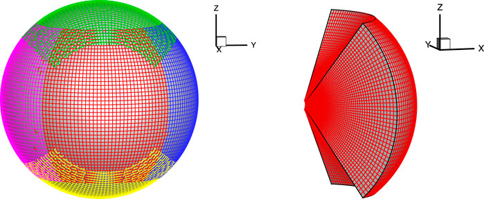
FIGURE 1. Six-component grid structure with partial overlap (left) and one-component mesh stacked in the r-direction (right). Adopted from Feng et al. (2010).
In both θ and ϕ directions, grid points are uniformly distributed: θi = θmin + (i − 1)Δθ, i = 1, …, Nθ − 1, ϕi = ϕmin + (i − 1)Δϕ, i = 1, …, Nϕ − 1, with Δθ = (θmax − θmin)/(Nθ − 2), Δϕ = (ϕmax − ϕmin)/(Nϕ − 2), where Nθ and Nϕ are the mesh numbers in latitudinal and longitudinal directions, respectively. In this paper,
There are two types of cells in our grid system after the computation area is partitioned. One is the hexahedron with six planes, shown in Figure 2A, and the other is the hexahedron with five planes and a spherical surface, shown in Figure 2B. The former denotes the interior computational cell and the latter the boundary cell near the inner boundary of the computational domain. The difference between them is that the boundary cell has one face lying on a spherical surface, and the associated area is labeled by the blue color.
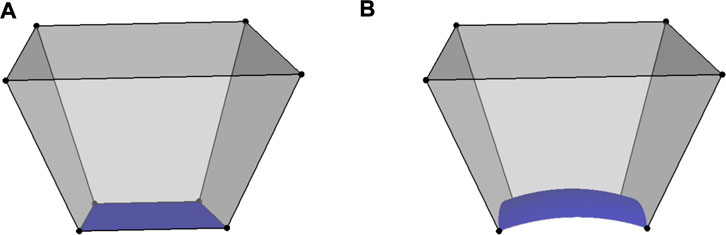
FIGURE 2. Hexahedral cells: (A) the interior cell, (B) the boundary cell.
3 Discontinuous Galerkin discretization
Introducing a pseudo-time derivative term to the Laplace’s Eq. 1 makes this equation into the following form:
where τ is the pseudo time. Obviously, the steady-state solution of Eq. 4 is the solution of the Laplace’s Eq. 1.
In DG method, the numerical solution of Eq. 4 in each cell of computational grid is represented as a linear combination of the local polynomial basis functions ψl(x):
Coefficients of this expansion, wl(τ), are the main unknown values in the DG methods. Usually, the DG method is termed as the DG (Pk) method if the variable Φ is represented using a piecewise polynomials of degree k. The number of basis functions, K, depends on the degree k of the expanded polynomials and the spatial dimensions d,
For DG (P2) case in three-dimensional space, K = 10, where P2 indicates that a piecewise polynomial of degree of two is used to compute the fluxes. The basis functions we choose are Taylor basis functions and are listed as follows. For cell Ωi,
where xi, yi and zi are the coordinates of the centroid of cell Ωi. Δxi, Δyi, and Δzi are the length scales in x −, y −, and z − directions, Δxi = 0.5 (xmax − xmin), Δyi = 0.5 (ymax − ymin), Δzi = 0.5 (zmax − zmin), and xmax, xmin, ymax, ymin, zmax, and zmin are the maximum and minimum coordinates in the local cell in three directions, respectively. And, the coefficients in Eq. 5, i.e., wl(τ), are the cell-average value and the scaled derivatives at the centroid of cell:
The weak formulation can be given through multiplying Eq. 4 by each basis function ψl(x), integrating it over cell Ωi with boundary Γi = ∂Ωi, and performing integration by parts:
where nij denotes the unit outward normal vector to the boundary Γi. Substituting Eq. 5 into Eq. 9 results in
The integral in Eq. 10 is computed exactly or approximately by using suitable numerical quadratures (Xia, 2013; Liu et al., 2017). To complete the DG space discretization, we need to define the numerical flux
In order to describe DDG method in a more convenient way, we introduce the following jump and average operators:
where the subscripts ⋅|L and ⋅|R denote the left and right states of a common face, respectively. With this definition, the x-direction, y-direction and z-direction components of flux for the DDG method can be given as
where β0 and β1 are regarded as two constant penalty parameters, and Δ is the characteristic face length. According to Cheng et al. (2016), we choose
where dij = (xj − xi, yj − yi, zj − zi) is the displacement vector from the centroid of Ωi to the centroid of Ωj. Hence, the numerical flux
At this moment, the flux Jacobian matrices for Φ and ∇Φ contributing to the diagonal block are respectively
and the flux Jacobian flux for Φ and ∇Φ contributing to the off-diagonal block are respectively
As for boundary face, the numerical flux
with
Therefore, at the outer boundary face,
where ΦB is given at the boundary specified by the Dirichlet condition. In this case, the numerical flux given by Eq. 19 becomes
and the flux Jacobian matrices for Φ and ∇Φ contributing to the diagonal block are respectively
At the inner boundary face,
where
and the flux Jacobian matrices for Φ and ∇Φ contributing to the diagonal block are
At an inner boundary face as a patch of the spherical surface, the normal direction of the boundary coincides with the radial direction. And, the outer normal direction of the inner boundary is negative to the radial direction, i.e., pointing to the interior of the Sun. As a result,
The spatial discretization in Eq. 10 leads to a system of ordinary differential equations:
where Mi denotes the mass matrix whose entries are
4 Implicit time integration
Using Euler implicit time integration, the semi-discrete system of ordinary differential Eq. 29 is rewritten as
where Δτ is the pseudo-time increment, and
where
with the superscripts i and j representing cell Ωi and Ωj, respectively.
Substituting Eq. 31 into Eq. 30, we obtain the following linear system over cell Ωi
where
For boundary cells, note that there are only five
where m denotes the iteration step, and ω the over-relaxation factor which is taken to be 1.3 in this work. This relaxation is performed to a specified tolerance, i.e.,
5 Numerical results
In this section, a 3D test case with the exact solutions is first performed to verify the effectiveness and accuracy of the developed DDG-PFSS code. Then we apply it to the extrapolation for solar potential magnetic field. All the computations in this study are accomplished on the TH-1A supercomputer from the National Supercomputing Center in TianJin, China, in which each computing node is configured with two Intel Xeon X5670 CPUs (2.93 GHz, six-core).
5.1 Validation of DDG-PFSS
To validate the solutions generated with the DDG-PFSS solver, we use an analytic solution, which is constructed according to Caplan et al. (2021), given by
The potential solution is given by
To test the code, we set the initial guess Φ = 0 and solve the system using the analytic Br of Eq. 40 as the inner boundary condition in the manner of Eq. 2 and using Eq. 3 as the outer boundary condition. The implicit solver is taken as converged when the L2 norm of the Φ residual is reduced by six orders of magnitude, i.e., ϵ = 1.0 × 10⁻⁶. For any solution variable s, the L2 norm error is defined as
where s(x) and s(x)exact are respectively the numerical and exact solutions evaluated at point x. Nglobal denotes the total number of the interior computational cells. Starting with a resolution of 40 × 12 × 12 × 6, we test the code with successively increased resolution. All runs are performed using 96 MPI processes. The results are presented in Table 1 and Figure 3. In Table 1, we present the L2 norm error of Φ on each level of meshes, as well as the order of accuracy for Φ. Between the coarser and finer meshes, following Lee, Ahn, and Luo (2018), the order of accuracy is measured as follows
with the superscripts “coarse” and “fine” denote the coarse mesh and fine mesh, respectively. Figure 3 displays the three-dimensional topologies of the gradient B = ∇Φ of Φ on the level of mesh with the resolution of 40 × 42 × 42 × 6. The left panel in this figure represents the analytic solution and the right panel the numerical solution. In these two panels, the starting points of the black lines representing ∇Φ are the same in order to make a visual comparison between the numerical solution and the exact solution. We see that the numerical solution is almost identical with the analytic solution, and the code exhibits the third-order accuracy as the mesh is gradually refined.
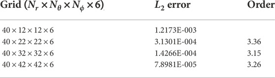
TABLE 1. L2 error and the order of accuracy for Φ.
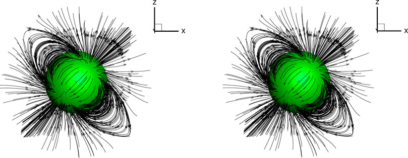
FIGURE 3. Depiction of the gradient ∇Φ of Φ in the test problem with the analytic solution: (left) analytic solution and (right) numerical solution.
5.2 Coronal potential magnetic field extrapolation
In this section, we extrapolate the coronal magnetic fields for CR 2060 (14 August To 10 September 2007) using the developed DDG-PFSS solver. The integral GONG synoptic magnetograms (in “mrmqs” format) are used as the inner boundary condition. These magnetograms are provided in the FITS format with the uniform 180 × 360, sin θ − ϕ mesh. With the help of MATLAB for reading the FITS files, we remesh the magnetograms to a uniform 181 × 361 latitude-longitude grid. In our DDG-PFSS solver, the magnetogram needs to be pre-processed, which is to remove the monopole. Therefore, the observed radial field Br (Rs, θj, ϕk) at the solar surface is corrected into
According to Schrijver et al. (2006) and Liu et al. (2011), we calculate some metrics that are used for checking the performance of the extrapolation solvers. They are Cvec, Ccs, Em and En, respectively, which are briefly defined below. Cvec is used to quantify the vector correlation,
where
where Mglobal is the total number of vectors in the domain to be calculated. Ccs = 1 means that
Em is a mean of the normalized vector errors,
The agreement is perfect when En and Em are equal to zero, which is unlike the first two metrics.
In Table 2, we show the metrics calculated using the extrapolated magnetic fields of the FDIPS and DDG-PFSS solvers. From the metrics, we see that the potential magnetic fields derived by the DDG-PFSS solver are slightly better than that obtained by the FDIPS method. Figure 4 presents the coronal magnetic field topologies obtained with (A) the SHE solver, (B) the FDIPS code and (C) the DDG-PFSS solver on the meridional plane of ϕ = 180°–0°. The backgrounds are colored with the radial component of magnetic field (Unit: G). The black lines represent the magnetic field lines, on which the arrowheads denote the directions. In order to make direct comparisons between these two numerical methods, the starting points at 1Rs of the magnetic fields are the same. By visual inspection, the large-scale magnetic topologies obtained from the three solvers are almost identical, such as the open-field regions, bipolar streamers and pseudo-streamers. In addition, we also present the comparison of the radial magnetic field between the two numerical solvers in Figure 5. The black, green and magenta lines represent the radial fields obtained by the SHE, FDIPS and DDG-PFSS solvers, respectively. The backgrounds are colored with the radial field of the SHE solver. From the low-latitude regions to the high-latitude regions, we can see that the radial field derived by the DDG-PFSS solver is closer to that of the SHE solver when compared to that derived by FDIPS. These results suggest the credibility of our established DDG-PFSS solver. In the following section, we continue to obtain other large-scale structures using our DDG-PFSS solver.
By tracing the magnetic field lines from the source surface to the photosphere, we obtain the coronal holes (CHs) regions, i.e., the footpoints of open magnetic field lines, which are shown in the dark regions in Figure 6. In Figure 6A, we present the 195 Å EUVI observation obtained by Solar Terrestrial Relations Observatory (STEREO)-A/Extreme Ultraviolet Imager (EUVI) instrument. In Figures 6B,C, we display the distributions of CHs derived from the SHE and DDG-PFSS solvers, respectively. From Figures 6B,C, we find no apparent differences between them. In addition, we calculate the CHs areas, shown as fraction of the Sun’s total surface area, which is about 13.77% for the SHE solver and 14.28% for the DDG-PFSS solver, respectively. From Figure 6A, we see that large CHs are mainly located in polar regions (polar CHs) during the solar minimum. The observed polar CHs and the extension of the southern polar CHs at about the longitudinal range of 90°–180° to lower latitude are well caught by the SHE and DDG-PFSS solvers. In observation, we also see some small and isolated CHs in the low-latitude regions, which we call as low-latitude CHs. Comparing the SHE- and DDG-derived results with observation shows that the configuration of low-latitude CHs is basically reproduced. However, some observed low-latitude CHs marked by red rectangles in Figure 6A are not captured by the SHE and DDG-PFSS solvers, which is also evidenced by Nikolić (2019). The red rectangles appearing in Figures 6B,C are located at the same positions as that shown in Figure 6A, with the purpose of making the visual comparison more convenient.
In Figure 7A, we show the synoptic map of polarized brightness (pB) observation at 2.5Rs. This synoptic map is created using data from the east limb of the SOHO/LASCO C2 instrument. The bright structures in the pB synoptic map may include the bipolar streamer and the pseudo-streamer (Wang, Sheeley, and Rich, 2007; Li, Feng, and Wei, 2021). The red line superimposed on this pB synoptic map denotes the magnetic neutral line (Br = 0) from the SHE solver, while the blue line represents the magnetic neutral line from the DDG-PFSS solver. From Figure 7A, we see that the blue line almost coincides with the red line and they are surrounded by the bright structures. Usually, the position of the magnetic neutral line is considered as the bipolar streamer belt. In comparison with the observation, the positions of SHE-derived and DDG-derived bipolar streamer belts agree reasonably with the observed pB bright structures. In addition, we use a streamer identification algorithm (Owens, Crooker, and Lockwood, 2014; Li, Feng, and Wei, 2021) to further identify the bipolar streamer and pseudo-streamer from the SHE- and DDG-derived results. That is, the regions where the parameter log (ds) > 1 are identified as bipolar streamer and pseudo-streamer belts. The parameter log (ds) is defined as
The PFSS model plays an important role in forecasting solar wind. Here, we take advantage of the Wang-Sheeley-Arge (WSA) model (Arge et al., 2003; Riley, Linker, and Arge, 2015) and the Arge-Pizzo kinematic evolution model (Arge and Pizzo, 2000; Riley and Lionello, 2011) to predict the solar wind speed vr at 1 AU. More specifically, by using the SHE- and DDG-derived magnetic fields we first configure the WSA model to obtain the solar wind speed at 30Rs, and then map the solar wind streams from 30Rs to 1 AU using the Arge-Pizzo kinematic evolution model. The general formulation of WSA model for solar wind speed is as follows
where a1 ∼ a8 are the empirical and adjustable parameters. fs represents the magnetic flux tube expansion factor and θb the minimum angular separation between an open magnetic field footpoint and its nearest coronal hole boundary. In Figure 8, we display the synoptic maps of two parameters fs and θb at 2.5Rs, in which fs and θb in Figure 8(A1, A2) are obtained by the SHE-derived magnetic fields, and those in Figure 8(B1, B2) from the DDG-derived magnetic fields. According to Riley and Lionello (2011), the Arge-Pizzo kinematic evolution model is expressed as
where Vi+1,j denotes the speed at ri+1 for longitude j. The iterative number in radial direction, which is applied between 30Rs and 1 AU, is set here to be 120. The mapped results are exhibited in Figure 9, which demonstrates the comparison between the OMNI data and the numerical results. The red lines in Figures 9A,B represent the mapped results based on the SHE solver and the DDG-PFSS solver, respectively. The black line denotes the OMNI data. The parameters in Eq. 48 which are chosen to produce the best match to the OMNI data are listed in Table 3.
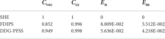
TABLE 2. Cvec, Ccs, En and Em for the extrapolated fields of the FDIPS and DDG-PFSS solvers.
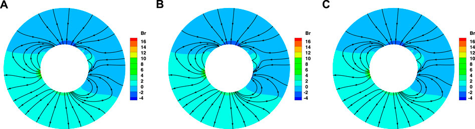
FIGURE 4. Topologies of the coronal magnetic fields on the meridional plane of ϕ =180°−0° from 1Rs to 2.5Rs, obtained with (A) the SHE solver, (B) FDIPS, and (C) the DDG-PFSS solver. In order to make direct comparisons between these two numerical methods, the starting points at 1Rs of the magnetic fields are the same.
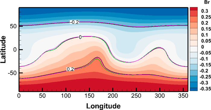
FIGURE 5. Radial magnetic field (Unit: G) at 1.8Rs for SHE (black lines), FDIPS (green lines) and DDG-PFSS (magenta lines). The backgrounds are colored with the radial field of the SHE solver. Negative and positive Br are denoted by blue and red color, respectively.
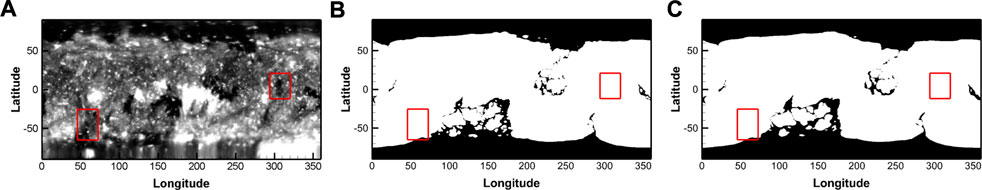
FIGURE 6. Synoptic maps of coronal holes: (A) observed by EUVI/SECCHI on board STEREO A; (B) obtained by the SHE solver; (C) obtained by the DDG-PFSS solver.
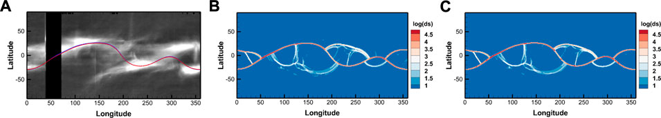
FIGURE 7. Synoptic map at 2.5Rs: (A) the pB at the east limb observed by SOHO/LASCO C2; (B) log (ds) obtained by SHE solver; (C) log (ds) obtained by DDG-PFSS solver. The red line in (A) denotes the magnetic neutral line (Br =0) from the SHE solver, while the blue line represents the magnetic neutral line from the DDG-PFSS solver.
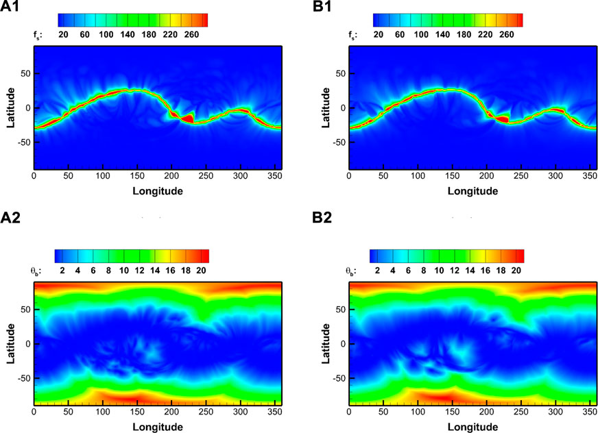
FIGURE 8. Magnetic flux tube expansion factor fs and the minimum angular separation between an open magnetic field footpoint and its nearest coronal hole boundary θb (Unit: degree) obtained by the SHE solver (A1, A2), and the DDG-PFSS solver (B1, B2).
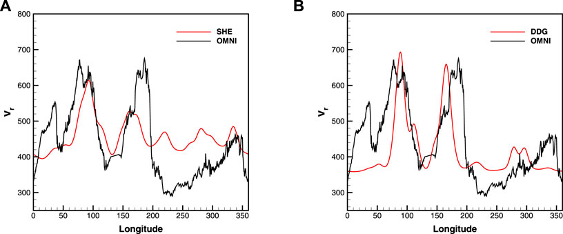
FIGURE 9. Comparisons between the interplanetary measurements from OMNI and the modeled radial velocity vr (km/s) based on the SHE solver (A) as well as the DDG-PFSS solver (B).

TABLE 3. The empirical parameters in WSA formula.
The comparison between the modeled and observational results suggests that the simulated results basically capture the structures of the high- and low-speed streams occurring in the observation, apart from the small deviation of the high-speed stream at about longitudinal range of 150°–190° shown in Figure 9A.
6 Conclusion
In this paper, we develop a DDG-PFSS solver for obtaining the potential magnetic field solutions. By introducing the pseudo-time into the Laplace’s Eq. 1, the Laplace’s equation is changed into a diffusion-like Eq. 4. The initial-boundary value problem for the modified equation is obtained to replace the boundary value problem for the Laplace’s equation. Then we apply the DG method to the space discretization of the modified equation. The steady-state solution of the initial-boundary value problem is the sought solution of the Laplace’s equation. As for the space discretization, we choose the DDG method to calculate the numerical flux across the interfaces because of its simplicity in implementation and efficiency in computation. In order to speed up the convergence, implicit backward Euler temporal discretization is applied to the pseudo-time system, and the resulting large linear system at each pseudo-time step is solved by the block SOR scheme.
To validate the DDG-PFSS solver, we test a problem with the exact solution, which demonstrates the effectiveness and third-order accuracy of the solver. Then we utilize this solver to calculate the global coronal magnetic field of CR 2060. The numerical magnetic fields generated by the DDG-PFSS solver are compared with those derived by the FDIPS code. The magnetic fields obtained by the SHE method serve as a reference solution. By comparison, we see that the magnetic fields derived by the DDG-PFSS solver are closer to that of the SHE solver. Finally, we also obtain the large-scale structures including CHs, bipolar streamer belts and pseudo-streamer belts using the DDG-PFSS solver. These structures have a good agreement with solar observations except for a few small and isolated low-latitude CHs. In addition, we obtain the solar wind speed at 1 AU using the WSA model and the Arge-Pizzo kinematic evolution model. The derived solar wind speed basically captures the structures of the high- and low-speed streams as occurred in the OMNI data. These results strongly suggest the credibility of our established DDG-PFSS solver. Compared to other numerical methods including the finite difference and finite volume methods, DDG discrete method possesses some attractive features, such as the compactness and the easy extension to high-order approximation. The numerical viscous flux defined by the DDG method is consistent and conservative (Liu and Yan, 2009). The most prominent feature of the DDG method is its simplicity in implementation and its efficiency in computation (Cheng et al., 2017). In a word, our DDG-PFSS model can be seen as an alternative contribution to computational space weather modelling in space physics.
The work is jointly supported by the National Natural Science Foundation of China (Grant Nos. 42030204, 41874202, 41731067, 41861164026, and 41531073), the strategic priority research program of CAS with Grant No. XDB09000000 and the Specialized Research Fund for State Key Laboratories. This work utilizes data obtained by the Global Oscillation Network Group (GONG) program, managed by the National Solar Observatory, which is operated by AURA, Inc. Under a cooperative agreement with the National Science Foundation. The data were acquired by instruments operated by the Big Bear Solar Observatory, High Altitude Observatory, Learmonth Solar Observatory, Udaipur Solar Observatory, Instituto de Astrofísica de Canarias, and Cerro Tololo Interamerican Observatory. The STEREO/SECCHI data are produced by a consortium of the NRL (United States), LMSAL (United States), NASA/GSFC (United States), RAL (United Kingdom), UBHAM (United Kingdom), MPS (Germany), CSL (Belgium), IOTA (France), and IAS (France). This work also utilizes data obtained by LASCO C2/SOHO. The OMNI data are obtained from the GSFC/SPDF CDAWeb interface at https://cdaweb.gsfc.nasa.gov/index.html. The work was carried out at the National Supercomputer Center in Tianjin, China, and the calculations were performed on TianHe-1 (A).
Data availability statement
The raw data supporting the conclusion of this article will be made available by the authors, without undue reservation.
Author contributions
XF put forward the idea of using DDG solver for obtaining the solar coronal potential magnetic field. XL implemented the code and run the results. All the authors are in involved in analysis of the numerical results and writing the manuscript.
Conflict of interest
The authors declare that the research was conducted in the absence of any commercial or financial relationships that could be construed as a potential conflict of interest.
Publisher’s note
All claims expressed in this article are solely those of the authors and do not necessarily represent those of their affiliated organizations, or those of the publisher, the editors and the reviewers. Any product that may be evaluated in this article, or claim that may be made by its manufacturer, is not guaranteed or endorsed by the publisher.
References
Altschuler, M. D., and Newkirk, G. (1969). Magnetic fields and the structure of the solar corona. Sol. Phys. 9 (1), 131–149. doi:10.1007/BF00145734
Arge, C. N., Odstrcil, D., Pizzo, V. J., and Mayer, L. R. (2003). “Improved method for specifying solar wind speed near the Sun,”. Editors M. Velli, R. Bruno, F. Malara, and B. Bucci (American Institute of Physics Conference Series), Sol. Wind Ten. 679. 190–193. doi:10.1063/1.1618574
Arge, C. N., and Pizzo, V. J. (2000). Improvement in the prediction of solar wind conditions using near-real time solar magnetic field updates. J. Geophys. Res. 105 (A5), 10465–10479. doi:10.1029/1999JA000262
Arnold, D. N. (1982). An interior penalty finite element method with discontinuous elements. SIAM J. Numer. Anal. 19 (4), 742–760. doi:10.1137/0719052
Bassi, F., Crivellini, A., Rebay, S., and Savini, M. (2005). Discontinuous Galerkin solution of the Reynolds-averaged Navier-Stokes and k − ω turbulence model equations. Comput. Fluids 34 (4), 507–540. Residual Distribution Schemes, Discontinuous Galerkin Schemes and Adaptation. doi:10.1016/j.compfluid.2003.08.004
Bassi, F., and Rebay, S. (1997). A high-order accurate discontinuous finite element method for the numerical solution of the compressible Navier-Stokes equations. J. Comput. Phys. 131 (2), 267–279. doi:10.1006/jcph.1996.5572
Caplan, R. M., Downs, C., Linker, J. A., and Mikic, Z. (2021). Variations in finite-difference potential fields. Astrophys. J. 915 (1), 44. doi:10.3847/1538-4357/abfd2f
Cheng, J., Liu, X., Liu, T., and Luo, H. (2017). A parallel, high-order direct discontinuous Galerkin method for the Navier-Stokes equations on 3D hybrid grids. Commun. Comput. Phys. 21 (5), 1231–1257. doi:10.4208/cicp.OA-2016-0090
Cheng, J., Yang, X., Liu, X., Liu, T., and Luo, H. (2016). A direct discontinuous Galerkin method for the compressible Navier-Stokes equations on arbitrary grids. J. Comput. Phys. 327, 484–502. doi:10.1016/j.jcp.2016.09.049
B. Cockburn, G. E. Karniadakis, and C. W. Shu (Editors) (2000). Discontinuous Galerkin methods (Berlin, Heidelberg: Springer). 978-3-642-64098-8. doi:10.1007/978-3-642-59721-3
Cockburn, B., and Shu, C. W. (1998). The local discontinuous Galerkin method for time-dependent convection-diffusion systems. SIAM J. Numer. Anal. 35 (6), 2440–2463. doi:10.1137/S0036142997316712
Dolejší, V., and Feistauer, M. (2015). Discontinuous Galerkin method. Cham: Springer. 978-3-319-19267-3. doi:10.1007/978-3-319-19267-3
Douglas, J., and Dupont, T. (1976). Interior penalty procedures for elliptic and parabolic Galerkin methods. Editors R. Glowinski, and J. L. Lions, 58, 207. doi:10.1007/BFb0120591
Feng, X. S., Yang, L. P., Xiang, C. Q., Wu, S. T., Zhou, Y. F., and Zhong, D. K. (2010). Three-dimensional solar wind modeling from the Sun to Earth by a SIP-CESE MHD model with a six-component grid. Astrophys. J. 723, 300–319. doi:10.1088/0004-637x/723/1/300
Feng, X., Li, X., Xiang, C., Li, H., and Wei, F. (2019). A new MHD model with a rotated-hybrid scheme and solenoidality-preserving approach. Astrophys. J. 871 (2), 226. doi:10.3847/1538-4357/aafacf
Hakamada, K., Kojima, M., Tokumaru, M., Ohmi, T., Yokobe, A., and Fujiki, K. (2002). Solar wind speed and expansion rate of the coronal magnetic field in solar maximum and minimum phases. Sol. Phys. 207, 173–185. doi:10.1023/A:1015511805863
Hartmann, R. (2006). Adaptive discontinuous Galerkin methods with shock-capturing for the compressible Navier-Stokes equations. Int. J. Numer. Methods Fluids 51 (9-10), 1131–1156. doi:10.1002/fld.1134
He, X., Wang, K., Feng, Y., Lv, L., and Liu, T. (2022). An implementation of mpi and hybrid openmp/mpi parallelization strategies for an implicit 3d ddg solver. Comput. Fluids 241, 105455. doi:10.1016/j.compfluid.2022.105455
Lee, E., Ahn, H. T., and Luo, H. (2018). Cell-centered high-order hyperbolic finite volume method for diffusion equation on unstructured grids. J. Comput. Phys. 355, 464–491. doi:10.1016/j.jcp.2017.10.051
Li, H., Feng, X., and Wei, F. (2021). Comparison of synoptic maps and PFSS solutions for the declining phase of solar cycle 24. JGR. Space Phys. 126 (3). doi:10.1029/2020JA028870
Liu, H. (2021). Analysis of direct discontinuous Galerkin methods for multi-dimensional convection–diffusion equations. Numer. Math. (Heidelb). 147, 839–867. doi:10.1007/s00211-021-01183-x
Liu, H., and Yan, J. (2009). The direct discontinuous Galerkin (DDG) methods for diffusion problems. SIAM J. Numer. Anal. 47 (1), 675–698. doi:10.1137/080720255
Liu, S., Zhang, H. Q., Su, J. T., and Song, M. T. (2011). Study on two methods for nonlinear force-free extrapolation based on semi-analytical field. Sol. Phys. 269, 41–57. doi:10.1007/s11207-010-9691-4
Liu, X., Feng, X., Xiang, C., and Shen, F. (2019). Hyperbolic cell-centered finite volume method for obtaining potential magnetic field solutions. Astrophys. J. 887 (1), 33. doi:10.3847/1538-4357/ab4b53
Liu, X., Xuan, L., Xia, Y., and Luo, H. (2017). A reconstructed discontinuous Galerkin method for the compressible Navier-Stokes equations on three-dimensional hybrid grids. Comput. Fluids 152, 217–230. doi:10.1016/j.compfluid.2017.04.027
Luo, H., Luo, L., Nourgaliev, R., Mousseau, V. A., and Dinh, N. (2010). A reconstructed discontinuous Galerkin method for the compressible Navier-Stokes equations on arbitrary grids. J. Comput. Phys. 229 (19), 6961–6978. doi:10.1016/j.jcp.2010.05.033
MacNeice, P., Jian, L. K., Antiochos, S. K., Arge, C. N., Bussy-Virat, C. D., DeRosa, M. L., et al. (2009). Validation of community models: 2. Development of a baseline using the wang-sheeley-arge model. Space weather. 7 (12), 1644–1667. doi:10.1029/2018SW002040
Nikolić, L. (2019). On solutions of the PFSS model with GONG synoptic maps for 2006-2018. Space weather. 17 (8), 1293–1311. doi:10.1029/2019SW002205
Nikolić, L., and Trichtchenko, L. (2012). Development of coronal field and solar wind components for MHD interplanetary simulations. Int. J. Environ. Chem. Ecol. Geol. Geophys. Eng. 6 (11), 698–702.
Nishikawa, H. (2007). A first-order system approach for diffusion equation. I: Second-order residual-distribution schemes. J. Comput. Phys. 227, 315–352. doi:10.1016/j.jcp.2007.07.029
Norquist, D. C., and Meeks, W. C. (2010). A comparative verification of forecasts from two operational solar wind models. Space weather. 8 (12). doi:10.1029/2010SW000598
Owens, M. J., Crooker, N. U., and Lockwood, M. (2014). Solar cycle evolution of dipolar and pseudostreamer belts and their relation to the slow solar wind. J. Geophys. Res. Space Phys. 119 (1), 36–46. doi:10.1002/2013JA019412
Riley, P., Linker, J. A., and Arge, C. N. (2015). On the role played by magnetic expansion factor in the prediction of solar wind speed. Space weather. 13 (3), 154–169. doi:10.1002/2014SW001144
Riley, P., and Lionello, R. (2011). Mapping solar wind streams from the sun to 1 au: A comparison of techniques. Sol. Phys. 270, 575–592. doi:10.1007/s11207-011-9766-x
Schatten, K. H., Wilcox, J. M., and Ness, N. F. (1969). A model of interplanetary and coronal magnetic fields. Sol. Phys. 6 (3), 442–455. doi:10.1007/BF00146478
Schrijver, C. J., De Rosa, M. L., Metcalf, T. R., Liu, Y., McTiernan, J., Régnier, S., et al. (2006). Nonlinear force-free modeling of coronal magnetic fields Part I: A quantitative comparison of methods. Sol. Phys. 235 (1-2), 161–190. doi:10.1007/s11207-006-0068-7
Stansby, D., Yeates, A., and Badman, S. T. (2020). pfsspy: A python package for potential field source surface modelling. J. Open Source Softw. 5 (54), 2732. doi:10.21105/joss.02732
Tóth, G., van der Holst, B., and Huang, Z. (2011). Obtaining potential field solutions with spherical harmonics and finite differences. Astrophys. J. 732, 102. doi:10.1088/0004-637X/732/2/102
Wang, Y. M., Sheeley, J. N. R., and Rich, N. B. (2007). Coronal pseudostreamers. Astrophys. J. 658 (2), 1340–1348. doi:10.1086/511416
Keywords: direct discontinuous Galerkin method, potential magnetic field, solar corona, numerical solution algorithm, pseudo-time derivative
Citation: Liu X, Feng X, Lv J, Wang X and Zhang M (2022) Direct discontinuous Galerkin method for potential magnetic field solutions. Front. Astron. Space Sci. 9:1055969. doi: 10.3389/fspas.2022.1055969
Received: 28 September 2022; Accepted: 08 November 2022;
Published: 01 December 2022.
Edited by:
Andrius Popovas, University of Oslo, NorwayCopyright © 2022 Liu, Feng, Lv, Wang and Zhang. This is an open-access article distributed under the terms of the Creative Commons Attribution License (CC BY). The use, distribution or reproduction in other forums is permitted, provided the original author(s) and the copyright owner(s) are credited and that the original publication in this journal is cited, in accordance with accepted academic practice. No use, distribution or reproduction is permitted which does not comply with these terms.
*Correspondence: Xueshang Feng, ZmVuZ3hAc3BhY2V3ZWF0aGVyLmFjLmNu