 Mehmet Aktukmak
 Zeyu Sun
 Monica Bobra2
 Tamas Gombosi
 Ward B. Manchester IV
 Yang Chen
 Alfred Hero
- 1Department of Electrical and Computer Engineering, University of Michigan, Ann Arbor, MI, United States
- 2W. W. Hansen Experimental Physics Laboratory, Stanford University, Stanford, CA, United States
- 3Department of Aerospace Engineering, University of Michigan, Ann Arbor, MI, United States
- 4Department of Climate and Space Sciences and Engineering, University of Michigan, Ann Arbor, MI, United States
- 5Department of Statistics, University of Michigan, Ann Arbor, MI, United States
In this paper, we consider incorporating data associated with the sun’s north and south polar field strengths to improve solar flare prediction performance using machine learning models. When used to supplement local data from active regions on the photospheric magnetic field of the sun, the polar field data provides global information to the predictor. While such global features have been previously proposed for predicting the next solar cycle’s intensity, in this paper we propose using them to help classify individual solar flares. We conduct experiments using HMI data employing four different machine learning algorithms that can exploit polar field information. Additionally, we propose a novel probabilistic mixture of experts model that can simply and effectively incorporate polar field data and provide on-par prediction performance with state-of-the-art solar flare prediction algorithms such as the Recurrent Neural Network (RNN). Our experimental results indicate the usefulness of the polar field data for solar flare prediction, which can improve Heidke Skill Score (HSS2) by as much as 10.1%1.
1 Introduction
Solar flares rapidly release magnetic energy stored in the Sun’s corona, which heats large areas of the surrounding atmosphere. The terrestrial impacts of flares can be serious, especially when they are high-intensity. Although weak flares have a limited impact on mankind, strong flares can disturb satellite communication and GPS-navigation systems, in addition to causing dangerous ionizing radiation exposure to astronauts orbiting the earth. Hence, timely prediction of solar flares, especially the strong ones, is desirable so that precautions can be taken. However, strong flares occur rarely as compared to weak flares, and the underlying mechanisms and the factors that trigger and determine the strength of the flares are not well understood. This makes the prediction of solar flares a complex task.
As the coronal field is anchored in the photosphere, the onset of flares has been linked to changes in the photospheric magnetic field (Sun et al., 2012; Wang et al., 2020). Consequently, it is reasonable to expect that photospheric magnetic fields in active regions (AR) may be useful indicators of flare-triggering mechanisms. The Helioseismic and Magnetic Imager [HMI; (Scherrer et al., 2012), (Hoeksema et al., 2014)] on Solar Dynamics Observatory [SDO; (Pesnell et al., 2012)] spacecraft has observed the photospheric magnetic field of the sun since 2010, taking high-resolution images with 1 arcsec spatial resolution and 720s cadence. From these magnetic field images, useful features are computed, known as Space-weather HMI Active Region Patches (SHARP) parameters, which are representative of the magnetic field’s scale, energy and complexity (Bobra et al., 2014). This time-series data has been successfully used for solar flare prediction for Solar Cycle 24 using machine learning algorithms (Bobra and Couvidat, 2015; Chang et al., 2017; Nishizuka et al., 2017; Florios et al., 2018; Jonas et al., 2018; Campi et al., 2019; Camporeale, 2019; Chen et al., 2019; Korsós et al., 2021). See also (Leka et al., 2019) for a comprehensive review.
Several supervised machine learning models have been proposed to predict solar flares from HMI observations. NOAA Geo-stationary Operational Environmental Satellites (GOES) flare list (Garcia, 1994) provides peak energy levels for each flare on a logarithmic scale separated into five flare intensity classes, labeled A, B, C, M, X, with A the weakest and X the strongest intensities. These can be used as categorical response variables in machine learning models for flare prediction. Such models use input features, such as HMI SHARP parameters, to apply off-the-shelf machine learning algorithms to predict the labels of the flares, including discriminant analysis (Leka et al., 2018), linear regression (Jonas et al., 2018), support vector machine (Bobra and Couvidat, 2015; Nishizuka et al., 2017; Florios et al., 2018), k-nearest neighbor (Nishizuka et al., 2017), random forests (Chang et al., 2017; Florios et al., 2018), multilayer perceptrons (Florios et al., 2018), and recurrent neural networks (Chen et al., 2019). Recently, the magnetogram images of the active regions have been used as features in deep learning models such as convolutional neural networks (CNN) [ (Huang et al., 2018), for prediction of flare intensity class. Ensemble models have also shown promise as a way of combining predictions of multiple models that use different data sources (Guerra et al., 2020; Sun et al., 2022).
Hale’s Polarity laws (Hale et al., 1919) for sunspots apprise that the polarities of the sunspots (distinguished in pairs with a leading/following counterpart from east to west) have a strong tendency to have the opposite pattern in the northern and southern hemispheres of the sun in a particular cycle. Moreover, the polarities of the spots of the present cycle are the opposite of the polarities in the previous cycle. Additionally, polar field reversals occur systematically at approximately the time of the solar cycle maximum (Babcock, 1959), with peak polar field values occurring at the time of the sunspot cycle minimum. Thus, the polar fields are 180° out of phase with the sunspot cycle. See Figure 1 for plots over time of the polar fields along with curves of sunspot number, unsigned AR flux, and AR latitude. Numerous works show how the polar field is reformed each cycle from a small fraction of active region flux, which is transported by meridional flows from mid-latitudes to the poles (Wang et al., 2005; Hathaway, 2015; Morgan and Taroyan, 2017).
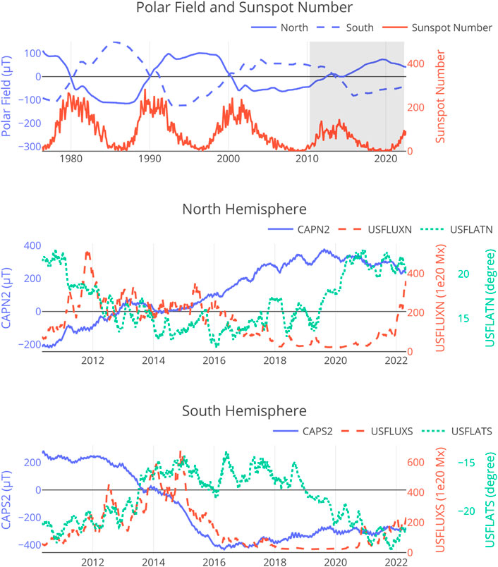
FIGURE 1. Top: The north and south polar strength and the monthly mean sunspot numbers plotted over 4 solar cycles. The shaded period is the time during which the HMI instrument has been generating data. Polar fields data are from the Wilcox Solar Observatory (Svalgaard et al., 1978; Hoeksema, 1995). Sunspot number data are from WDC-SILSO, Royal Observatory of Belgium, Brussels. Middle: Solar cycle variation of the north polar field strength (CAPN2), AR unsigned flux (USFLUXN), and flux-weighted AR latitude (USFLATN) obtained from HMI data. The unsigned flux in the northern hemisphere (USFLUXN) is positively correlated with the north polar fields (CAPN2), suggesting the inclusion of polar field data as additional features in a machine learning flare prediction model can potentially improve prediction accuracy. Bottom: Similar to the Middle panel but for the Southern Hemisphere of the sun.
It has been demonstrated that the strength of the sun’s polar fields can be used to predict the next solar cycle’s sunspot intensity based on the understanding of the sun’s magnetic dynamo (Dikpati and Gilman, 2006; Hiremath, 2008; Upton and Hathaway, 2013)2. Weak polar fields at the end of Cycle 23 motivated the authors of the 2005 paper (Svalgaard et al., 2005) to forecast a weak Solar Cycle 24. Indeed, Solar Cycle 24 has been the weakest solar cycle in a century. To graphically illustrate the strong association between polar fields and sunspot activity, we the polar fields and monthly mean sunspot number over four solar cycles in the top panel of Figure 1. It can be observed the magnitude of the difference between the two polar fields at the solar minimum is a good indicator of the intensity of the subsequent cycle.
The relation between polar fields and AR magnetic fields is more intricate, involving complex physical mechanisms. This is better observed with higher temporal resolution and in an AR-localized manner. The middle and bottom panels of Figure 1 shows how polar fields interact with total unsigned flux and latitudinal distribution of ARs in the northern and the southern hemisphere, respectively, during the period that HMI has been in operation (the shaded area in the top panel of Figure 1). The data are collected from the data product hmi.meanpf_720s, available at the Joint Science Operations Center (JSOC). The north and south polar field strengths are represented by CAPN2 and CAPS2, respectively, which correspond to the mean radial field within latitudes N60-N90 and the mean radial field within latitudes S60-S90. The unsigned AR flux can be well approximated by the unsigned flux in between S40 and N40, since flux is concentrated in ARs which are mostly located in those latitudes. Specifically, for the northern hemisphere, we compute the unsigned AR flux (USFLUXN) and unsigned-flux-weighted latitude (USFLATN) via.
where FLUXN_P (FLUXN_N) is positive (negative) flux between N0-N40 above a fixed threshold, and FLATN_P (FLATN_N) is positive (negative) flux weighted latitude between N0-N40. Similar quantities are computed for the southern hemisphere as well. The active regions’ locations follow the well-observed butterfly diagram of sunspots, starting approximately ± 40° latitude at the beginning of a solar cycle, and gradually drifting towards the equator as the cycle progresses. At the cycle minimum, there is an overlap of the old (near the equator) and new (near ± 40°) cycle spots. These trends can be observed from the lower two panels of Figure 1. It is worth noting that the rapid transition in AR latitude at the depth of solar minimum provides a strong signature of the solar cycle when the total flux and polar fields show the lowest variation with time. These strong and complex relations between polar fields and AR fields suggest supplementing SHARP features with HMI polar field strength may improve the prediction of AR-localized flare intensity levels. This is our main motivator for applying machine learning flare prediction approaches to the combined data.
In summary, we validate the usefulness of polar field features in predicting solar flares. The motivation is to assess whether combining SHARP keywords with polar field features can improve solar flare prediction performance or not. To this end, we design an experiment in which there are multiple possible ways of incorporating polar field data, four different machine learning models, and different train-test-validation splitting methods for each algorithm. In addition, we design a novel mixture of experts model tailored for incorporating polar field data for solar flare prediction context. Our experimental results indicate that polar field data can improve solar flare prediction performance. They also show that mixture of experts modeling is a simple yet effective alternative for combining polar field data and SHARP parameters, which can give similar or better performance to much more complicated neural network-based algorithms.
The rest of this paper is organized as follows. In Section 2, we describe how we incorporate multiple data sources into flare prediction algorithms, and we introduce several data-splitting methods for assessing the performances of the models. In Section 3, we formally define the machine learning models that are compared in this study including the new mixture of experts model. In Section 4, we describe the experimental setup in detail and present our results.
2 Data preparation
There are three distinct data sources we exploit in this study, namely, SHARP, GOES, and SPF datasets. The SHARP dataset provides parameters computed from the magnetograms produced by the HMI (See Table A3) instrument. These parameters are associated with the active regions that occurred from 2010 to 2020. We use the data product hmi.sharp_cea_720s, which contains definitive data in Cylindrical Equal-Area (CEA) coordinates and is available at the Joint Science Operations Center (JSOC). The GOES dataset includes solar flare event records measured by Geostationary Operational Environmental Satellites (GOES). This dataset can be downloaded using the SunPy package3 and it covers the HMI time period from 2010 to 2020. The flare events are labeled by A, B, C, M, and X, based on the peak intensity of X-ray flux measures. The Solar Polar Fields (SPF) dataset consists of two solar polar field features, namely, CAPS2 and CAPN2. These features correspond to the mean radial field in latitudes N60-N90, and the mean radial field in latitudes S60-S90, respectively. Both HMI and MDI instruments record these features, which can also be downloaded from JSOC. The MDI instrument was operational from 1996 to 2010 and the HMI has been operational since 2010.
2.1 SPF preprocessing
The noise levels on CAPS2 and CAPN2 features are significant, and the noise level is different in the HMI and MDI instruments. Hence, we consider smoothing by using a Kalman filter to filter out noise over these features. Note that the variance over the time series data is not solely due to noise. There is strong yearly modulation due to the Earth-solar B0 angle, where the solar rotation axis varies by ±7°. Furthermore, there is strong 27-day modulation due to solar rotation.
We implement the Kalman filter using the local level model (Murphy, 2012) where the state transition and observation models are defined as follows:
where yt is the raw noisy observation at time t, at is the filtered data, and
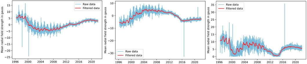
FIGURE 2. Raw (blue curve) and Kalman filtered (red curve) polar field features. Polar field strengths at the north pole CAPN2, south pole CAPS2, and the solar cycle approximation, defined as the unsigned polar field difference |CAPS2(t) − CAPN2(t)|, are shown in the left, middle, and right-hand panels respectively. The data source switched from MDI to HMI in 2010, which is accompanied by a visually obvious reduction in noise. The HMI data source has lower noise due to its high resolution.
2.2 Observation preprocessing
In this section, we describe how we use the HMI SHARP dataset and the GOES flare intensity labels to construct the training and test data for our discriminative machine learning algorithms, developed in the next section. Our Preprocessing steps for these data follow the approach in (Chen et al., 2019; Jiao et al., 2020; Sun et al., 2022).
We only include ARs having unique NOAA AR numbers (Jiao et al., 2020) into our training set. We eliminate low-quality observations by excluding ARs that occur outside of range ± 70 relative to the central meridian (Chen et al., 2019). Similarly to (Bobra et al., 2014; Chen et al., 2019) we focus on predicting whether a solar flare from a given active region will be strong (M/X class) or weak (B class). The A-class flares are excluded as they are almost indistinguishable from the background radiation. The C-class flares are frequently missing their NOAA AR numbers in the GOES database, making their locations difficult to track (Bobra and Couvidat, 2015). Exclusion of A and C flares and combining M and X class flares together creates a binary classification problem that enables the comprehensive comparative computational analysis we report in Section 4. This is a step along the way of establishing the value of polar field data for the more complex classification task of classifying between the five labels A, B, C, M, X, which is worthwhile of future study.
As in (Jiao et al., 2020), the class label of an AR is designated as the strongest flare occurring in a 24-h prediction period, according to the GOES database. Thus an AR is assigned a B label if there are no M/X flares within 24 h, while it is assigned label M/X otherwise. This is accomplished as follows. For each of the flares occurring in an AR, variables are extracted from the time segment spanning a 24-h time period from 48 h to 24 h before the occurrence of the flare. Since the cadence of the HMI observations is one sample every 12 min this yields a matrix of 22 SHARP predictor variables defined over 120-time points. If, for a given flare, the corresponding predictor variables have NaN values no class prediction is generated and we omit the flare from our analysis. Furthermore, in our analysis, we do not use any flare labels in the first 24 h of the beginning of an ARs since such flares would have no associated observed predictor variables. Once these omissions are taken into account, the total number of observations (predictor variables-label pairs) is 2,663. See Table 1 for a summary of our set of SHARP features.
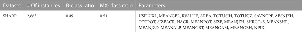
TABLE 1. SHARP dataset statistics after preprocessing step. See Appendix Table A3 for the definitions of the keywords.
2.3 Train-validation-test splitting
We consider three different methods for splitting the set of AR samples into train-test sets. In all three methods, we split the AR’s into 80% train and 20% test samples. 1) Instance-based splitting. The indexes of the splits are generated randomly without replacement. This split can measure the goodness-of-fit but is prone to information leakage when the observations of a particular AR are scattered among the splits (Sun et al., 2022). 2) AR-based splitting. AR numbers are used instead of the observation indexes for random index generation. This split prevents the information leakage that happens in Random splitting but may introduce another form of information leakage due to sympathetic flaring between neighboring ARs (Sun et al., 2022). 3) Month-based splitting. The timestamps are used to split the sets in terms of months with the same ratio. This split can also measure the goodness of fit and is closer to the operational forecasting setting. Each feature in the dataset is normalized over the time windows of the training data. Specifically, for each AR the mean and standard deviation of each feature is computed over the time points of the training sample. Then for each AR and each variable, the mean is subtracted and the result is divided by the standard deviation for both training and test samples.
3 Prediction algorithms
We consider four machine learning models that can exploit polar field features for the flare prediction task: 1) Logistic Regression (LR); 2) Mixture of Experts (MOE); 3) Multi-Layer Perceptron; 4) Recurrent Neural Network.
3.1 Logistic regression
Logistic Regression (LR) is a model for which the conditional distribution of the response variable as a Bernoulli distribution conditioned on the features of an AR sample in the case of binary classes, and categorical (multinomial) distribution for multiple classes. Specifically, for the binary case, LR models the conditional distribution of the response variable as
where i indexes the data points, yi = {0, 1} denotes the response variable (i.e., flare class), and xi corresponds to the SHARP parameters. The model parameters Θ are estimated from the training set by using Maximum Likelihood Estimation (MLE). In particular, the MLE objective over the N AR samples
which is convex in Θ, and has a unique solution. We use LBFG-S (Liu and Nocedal, 1989) to optimize the model parameters. In order to introduce polar field features to LR, a simple approach is to concatenate them with the SHARP parameters and apply the algorithm with these augmented features.
3.2 Mixture of Logistic regressions
A richer family of conditional distributions can be obtained by using a mixture of experts (MOE) framework (Yuksel et al., 2012). For classification tasks, each expert is an LR model. The predictions of the experts are mixed probabilistically according to mixture coefficients, which are obtained by using another linear model called the gating function. The output of the gating function is constrained to be a simplex to support proper mixing coefficients. This is achieved by using a Softmax function
Let zi denote a K dimensional categorical valued latent variable that indicates which expert is active for data point (AR) i, where K is the total number of experts initialized. The categorical conditional distribution of the latent variable zi induced by the gating function is given as
where ti denotes the polar field features associated with data point i, and V represents the gating function parameters that map features to the logits of the categorical distribution. After the softmax function, we obtain proper mixture coefficients for data point i. Since the experts are logistic regression models, their conditional distributions are given as
where Θk denotes the parameters of the expert k. The marginal likelihood of this model can be computed by integrating out the latent variables as follows
The objective is to maximize marginal log-likelihood with respect to the logistic regression and gating function parameters. The Expectation Maximization algorithm is a suitable optimization method for latent variable models. The algorithm optimizes the expected complete data log-likelihood (ECLL) instead of marginal, where the former forms a lower bound for the latter. There are two alternating steps, E and M steps. In the E-step of the algorithm, the posterior distributions of the latent variables are computed and their expectations are plugged into the complete data log-likelihood to obtain ECLL. Subsequently, the ECLL is maximized with respect to the model parameters in the M-step. These steps are iterated until ECLL converges. For the mixture of experts model, the ECLL is given as
where we replace the explicit expression of the prior distribution of mixture coefficients. rik denotes the posterior distribution of zi, which can be computed as
in the E-step of the EM algorithm. Replacing the posterior in the complete data log-likelihood, we get parameter-specific objectives to optimize in the M-step. Specifically, for the model parameters of the experts, the objective becomes
which can be computed by using any gradient-based optimizer. Note the similarity of this objective with Eq. 6. Hence, the former corresponds to weighted Logistic Regression. For the parameters of the gating function, the objective takes the following form
which is also similar to the Logistic Regression objective in Eq. 6 except that the response variable is simplex instead of discrete. This objective can also be maximized with any gradient-based optimizer. We use LBFG-S for all gradient-based optimization tasks. In summary, the E-step constitutes computing posterior distributions of the latent variables given the current values of the parameters by using Eq. 11, the M-step constitutes maximizing Eq. 12 and Eq. 13 with respect to Θk and V. When Eq. 10 converges, the iterations are halted. If we don’t use polar field features, mixing coefficients are unconditional as analogous to Gaussian Mixture Models.
3.3 Multi-layer perceptron
The Multi-layer Perceptron (MLP) is a non-linear discriminative classification model. MLPs can be more powerful than their linear counterparts when the interactions between the features and the response variables can not be explained by linear decision boundaries. An MLP can be obtained by stacking multiple fully connected layers. Each layer performs an affine transformation, and subsequently applies a deterministic non-linear function, e.g., softmax, relu, tanh. Stacking multiple layers result in a complex deterministic function of the input features. Let fΘ denote this function with the exception that the last layer does not apply any activation functions. Here, Θ represents the set of the affine transformation parameters of all the layers. Then, the conditional distribution for a binary classification task is given as
where the loss function is the same with LR as in Eq. 6.
The maximization of this distribution can be achieved by using a back-propagation algorithm (Hecht-Nielsen, 1992). We consider using polar field features as the additional features by concatenating them with the SHARP parameters.
Analogously to LR, a mixture of MLPs can be constructed by initializing multiple MLPs and mixing them using the probabilistic objective given in Eq. 9 (Bishop, 1994). However, in the MLP case, the EM algorithm is no longer applicable. Fortunately, back-propagation can still be used to maximize the objective. Similar to the Mixture of Logistic regression, a separate gating function can be initialized that maps polar field features to the mixture coefficients. This function can be linear or non-linear (MLP). In our experiments, we did not observe a significant performance change for Mixture of MLPs over NN-Augmented. Hence, we omit the Mixture of MLPs in this study.
3.4 Recurrent neural network
The aforementioned algorithms do not take the sequential nature of the observations into account. A more principled approach would model temporal data by assuming Markov chains between the consecutive inputs or outputs. Recurrent Neural Networks (RNN) do that by forming a first-order Markov chain between the hidden units. RNNs have shown significant success for sequential data modeling, and LSTM, a variant of RNNs, achieves state-of-the-art performance in flare forecasting from time series SHARP data (Chen et al., 2019; Liu et al., 2019; Sun et al., 2022). For this study, we use a particular version to classify the sequences of the input observations, also known as time series classification. The conditional distribution of the model is given as:
which implies that the observed label is dependent on a sequence of input data points. The length of the sequence is denoted as T and is a hyper-parameter of the model. The log-likelihood function associated with the RNN model is
where Θ represents the parameters of the model and can be optimized by using the backpropagation algorithm and T = 120 is the number of temporal samples in each AR training sample. The polar field features are incorporated as additional input features by concatenating them with the SHARP parameters.
4 Experiments
4.1 Configurations
The 4 algorithms described in Section 3 were compared in terms of relative performance improvements when adding the polar field to the SHARP features. Our SHARP dataset consists of 2,663 samples with 22 parameters over 120 time points. As described above we consider 3 different data splits: instance-based, AR-based, and month-based. For polar field features, we create two modes: raw CAPS2 and CAPN2 used as two separate input features; and cycle, where the absolute difference of CAPS2 and CAPN2 is used as a lower dimensional solar cycle approximation (see Figure 3). We also consider smoothed versions of CAPS2 and CAPN2 by using the Kalman filter, and unfiltered versions of these features. Hence, the total number of experimental configurations is 12 if we don’t use the polar field feature, and 48 otherwise. We perform cross-validation by using training splits for each configuration to select the regularization strengths of the algorithms. Also, we perform 20 runs to assess the significance of the accuracies. Hence, the total number of runs is around 7k.
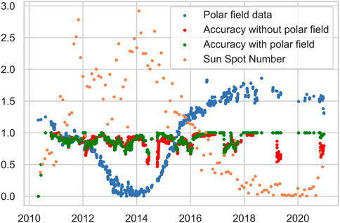
FIGURE 3. The classification accuracy curves of MOE with and without using polar fields data w.r.t. to the sunspot number when the splitting method is instance-based. Cycle approximation with filtered data is used as input. The curves are moving averaged over 90 days. The incorporation of the data substantially improves classification accuracy in some portions of the solar cycle.
4.2 Tuning
The hyper-parameters of the machine learning algorithms must be tuned for fair performance comparison. Cross-validation on the training set is used to select the best hyper-parameters for each experimental configuration. First, the training dataset is divided into 5 folds. The first fold is held out for measuring the performance of a hyper-parameter setting while the rest are used for training the algorithm. Then the hold-out set is alternated one by one so the total number of empirical realizations of performance for each hyper-parameter setting is 5. The average of these 5 values is then used as the score of that particular setting. We use the Heidke Skill Score HSS2 (Cohen, 1960; Bobra and Couvidat, 2015) for quantifying performance, which is defined as follows:
where TP, TN, FP, and FN correspond to true-positive, true-negative, false-positive, and false-negative values computed from binary classification predictions and ground truth, respectively.
All the algorithms studied were implemented with the standard L2-norm regularization approach to minimize overfitting. Regularization is accomplished by a penalty method, where the sum of the L2-norm squared of each parameter vector is weighted by a regularization parameter and added to the log-likelihood functions of each of the predictor models discussed in Section 3. The regularization parameters are tuned to optimize the performance of each algorithm. For LR, MLP, and RNN, the regularization strength is a single scalar that is common for all the elements of the parameters. The grid search range for this scalar is chosen as [0.1, 1, 10]. For MOE, we have separate parameters for the gating function and the experts. We use one scalar regularization parameter for the parameters of the gating function, and another for the parameters of the experts. The grid range for these two hyper-parameters is similarly determined as [0.1, 1, 10].
In addition to regularization tuning, the mixture model has a hyper-parameter associated with the total number of experts being initialized. The grid search range for this hyper-parameter is set as (Cohen, 1960; Bishop, 1994; Bobra et al., 2014; Bobra and Couvidat, 2015; Campi et al., 2019; Camporeale, 2019; Chen et al., 2019). We fix the network structure of RNN and MLP. In particular, 32 nodes with one hidden layer are initialized for both models.
4.3 Significance assessment
To assess the significance of the results, we repeat each experimental configuration n = 20 times with and without using polar field data. We then compute p-values from one-sided paired t-tests. The t-statistic is computed as
4.4 Results
The results are compiled in Table 2. We report HSS2 computed on the test set as the performance metric. For each algorithm, we only keep the configurations with statistically significant performance improvement due to the incorporation of polar field data, where significance is defined as a p-value less than 0.05 (5% level) of a one-sided paired t-test of equal mean performance, computed from 20 runs. For the LR model, there are two configurations that exhibit significant performance differences when polar field features are incorporated. Both of them imply that performance improves with the incorporation polar field. Particularly when we use unfiltered cycle approximation for the polar field features and filtered raw features, we obtain performance boost for the month (8.2%) and instance-based splits (1.5%), respectively. For the MOE model, there are four significant cases with all of them yielding performance improvements. The performance boost is up to 9.9%. The model can exploit the polar field augmented data regardless of filtering and preprocessing options when the splits are instance and month based to improve flare classification performance. For filtered raw features, the MLP improves performance on instance-based splitting by 4.9% and non-filtered cycle approximation on month-based splitting improves by 7.0%. The RNN performance is boosted regardless of filtering, preprocessing, and splitting options for four significant cases, achieving improvements as high as 10.1%. In summary, out of 12 significant cases for four algorithms, 11 of them provide performance increase, which suggests that polar field features to have high potential to improve solar flare prediction performance.
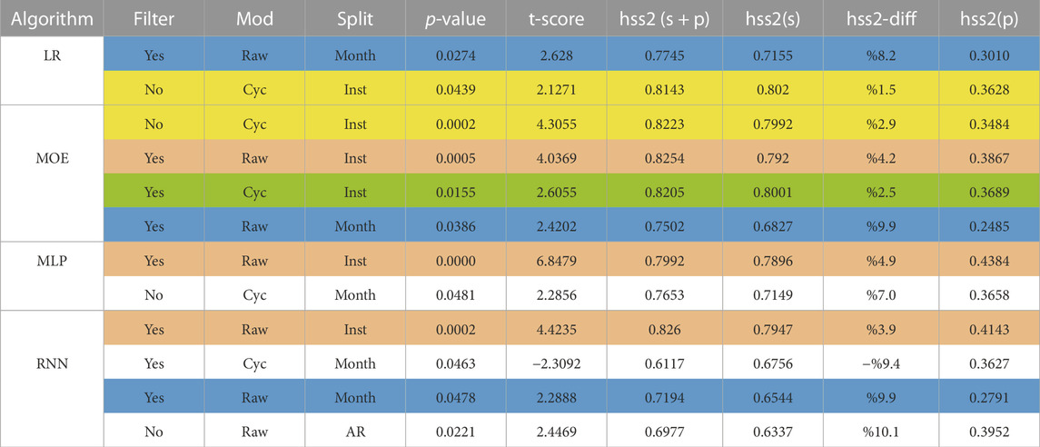
TABLE 2. Table of statistically significant (p-value ≤ 5%) performance improvements due to adding polar field features to SHARP features, The hss2 skill score argument (p) means only polar fields data, (s) means only SHARP parameters, and (s + p) means both data sources are used as input to the algorithms. (diff) is the mean hss2 score percentage difference when the polar field is incorporated in addition to SHARP parameters. The highlight colors in the table specify the common configurations where MOE achieves statistically significant performance improvements due to adding the polar field. The full tables including the statistically non-significant configurations are provided in the supplementary.
The column hss2(p) shows the prediction performance of the algorithms when only polar field data is used. The results indicate that sole use of polar field data gives poor skill scores, which is less than half of those of the SHARP data alone, for solar flare prediction. However, the hss2(p) scores are far from zero since solar cycle intensity and polar fields are correlated, as discussed in Section 1. Solar cycle intensity affects the expected intensities of the flares in particular time frames. Due to this connection, one can expect that coarse predictions about the classes of solar flares can be made with polar field data since it captures information about the solar cycle.
For the MOE model, the solar cycle dependency of the classification accuracy is shown in Figure 3 by repeating five experiments using instance-based splitting. We plot sunspot numbers, polar fields data (cycle approximation), accuracy without polar fields data, and accuracy with polar fields data. The classification accuracy curves are smoothed out with a 90-day moving average. We observe that MOE can exploit polar field data to improve classification accuracy in some parts of the solar cycle. The average classification accuracies over the whole HMI period are 0.88 and 0.91 for without and with polar field data, respectively. One can also observe the high negative correlation between the sunspot number and the curve of the polar field, which is computed as -0.86.
Finally, we compare the performance improvements of the models in Table 2. Only those configurations for which the p-value was significant at a level of 5% are shown. Among all algorithms MOE stands out as the only one to attain highly significant performance improvement (p-value = 0.0002) when no Kalman filtering is used, the magnitude difference north and south polar field data are used (the solar cycle approximation), and the splitting is instance based. MOE, MLP, and RNN, all have highly significant performance improvement when the polar field data is smoothed using the Kalman filter, the northern and southern polar fields are not combined into a cycle approximation (raw) and the split is instance based. Overall, among the five common configurations for which MOE achieves statistically significant improvement at the 5% level, MOE exhibits better performance in three of them, comparable performance in one of them, and slightly worse performance in the other one. We conclude that MOE is a promising machine learning model that can incorporate polar field data to improve flare classification accuracy.
We conclude this section by discussing some of the limitations of this study, which create opportunities for future research. Firstly, while we have established the value of polar field data when the train vs. test data split is randomized over time, our conclusions may not translate to operational flare forecasting where train and test data are drawn from past and future observations, respectively. We could not implement such a temporally defined data splitting to train our algorithms due to the fact that HMI data is currently available only over a single solar cycle. Secondly, it is possible that we could strengthen our conclusions by accounting for the temporal and longitudinal correlations of the polar field and active region magnetograms. In particular, instead of summarizing the polar field as the difference between both north and south polar fields (CAPN2 and CAPS2) we might be able to improve our model by incorporating the spatial coordinates of the active regions and independently applying CAPN2 and CAPS2 to the northern and southern hemisphere active regions, respectively (see Figure 1). Alternatively, it might be beneficial to incorporate a dynamic physics-based prediction model to account for dependencies between past active region activity and present polar field intensity. Furthermore, the added value of using polar field data may increase if we expanded the feature dimension to use the higher resolution HMI image data instead of just SHARP summarized data of active regions.
5 Conclusion
In this paper, we investigated the utility of the sun’s north and south polar field strength for improving solar flare prediction from HMI data. We presented an extensive experimental study, that analyzes multiple ways of preprocessing schemes for polar field data, several machine learning models that can incorporate this additional data source, diverse experimental conditions, and multiple splitting methods. The mixture of experts model was introduced for this particular global data incorporation task Our experimental results showed that polar field data is valuable for improving classification performance in multiple configurations. Additionally, we demonstrated that the proposed mixture of experts model can effectively supplement SHARP parameters with polar field data with for improved flare prediction.
The results suggest a causal connection between isolated ARs captured in the SHARP data and the global magnetic field captured in the polar field. The connection could come through the polar field itself due to the causal relationship between the event of decaying ARs and the subsequent drift of enhanced field towards poles. Hence, AR activity is anti-correlated to the polar field with a certain phase shift. In this study, we find that the probability of individual flare events is also correlated to the total sunspot number through the solar cycle, which closely follows the polar field strength. To put this work in context we point out that the polar field data has been used to inform solar cycle predictions with reasonable accuracy (Pesnell, 2012; Pesnell, 2020). We believe this work represents the first time the global field has been used to augment the prediction of solar flares.
In future work, there are several promising directions to enhance current results. The phase shift between the solar cycle/AR activity and polar field strengths can be estimated jointly by developing a more sophisticated model that can estimate and take into account phase shifts to improve prediction performance. The ARs in the northern and southern hemispheres can be modeled separately for more focused predictions. The correlation between the polar field strengths and other global indicators such as total active region area and flux-weighted latitude at a certain time can be investigated and possibly utilized for improved prediction performance. Finally, the data and the model may be further refined by using HMI high-dimensional image data instead of SHARP features.
Data availability statement
Publicly available datasets were analyzed in this study. This data can be found here: http://jsoc.stanford.edu/data/hmi/sharp/; http://jsoc.stanford.edu/data/hmi/polarfield/.
Author contributions
MB, AH, and YC provided the conceptualization, AH suggested the mathematical modeling approach and supervised the research. MA developed the model and performed the statistical analysis and wrote the first draft of the paper, ZS identified the data resources, helped download them, and advised MA on the analysis. YC, WM, and TG provided feedback on the research results and suggested improvements to the paper. WM made physical interpretation of the model results. All authors were involved in reviewing and approving the final manuscript.
Funding
This work was partially supported by NASA DRIVE Science Center grant 80NSSC20K0600, NASA grant 80NSSC18K1208, and DOE grant DE-NA0003921.
Conflict of interest
The authors declare that the research was conducted in the absence of any commercial or financial relationships that could be construed as a potential conflict of interest.
Publisher’s note
All claims expressed in this article are solely those of the authors and do not necessarily represent those of their affiliated organizations, or those of the publisher, the editors and the reviewers. Any product that may be evaluated in this article, or claim that may be made by its manufacturer, is not guaranteed or endorsed by the publisher.
Supplementary material
The Supplementary Material for this article can be found online at: https://www.frontiersin.org/articles/10.3389/fspas.2022.1040107/full#supplementary-material
Footnotes
1Acknowledgements: The authors would like to thank Graham Barnes for his valuable comments and suggestions. This work was partially supported by NASA DRIVE Science Center grant 80NSSC20K0600 and W. Manchester was partially supported by NASA grant 80NSSC18K1208.
2https://ntrs.nasa.gov/api/citations/20130013068/downloads/20130013068.pdf.
References
Bobra, M. G., and Couvidat, S. (2015). Solar flare prediction using sdo/hmi vector magnetic field data with a machine-learning algorithm. Astrophys. J. 798 (2), 135. doi:10.1088/0004-637x/798/2/135
Bobra, M. G., Sun, X., Todd Hoeksema, J., Turmon, M., Liu, Y., Hayashi, K., et al. (2014). The helioseismic and magnetic imager (hmi) vector magnetic field pipeline: Sharps–space-weather hmi active region patches. Sol. Phys. 289 (9), 3549–3578. doi:10.1007/s11207-014-0529-3
Campi, C., Benvenuto, F., Maria Massone, A., Shaun Bloomfield, D., Georgoulis, M. K., and Piana, M. (2019). Feature ranking of active region source properties in solar flare forecasting and the uncompromised stochasticity of flare occurrence. Astrophys. J. 883 (2), 150. doi:10.3847/1538-4357/ab3c26
Camporeale, E. (2019). The challenge of machine learning in space weather: Nowcasting and forecasting. Space weather. 17 (8), 1166–1207. doi:10.1029/2018sw002061
Chang, L., Deng, N., Wang, J. T. L., and Wang, H. (2017). Predicting solar flares using sdo/hmi vector magnetic data products and the random forest algorithm. Astrophys. J. 843 (2), 104. doi:10.3847/1538-4357/aa789b
Chen, Y., Manchester, W. B., Hero, A. O., Toth, G., Benoit, D., Zhou, T., et al. (2019). Identifying solar flare precursors using time series of sdo/hmi images and sharp parameters. Space weather. 17 (10), 1404–1426. doi:10.1029/2019sw002214
Cohen, J. (1960). A coefficient of agreement for nominal scales. Educ. Psychol. Meas. 20 (1), 37–46. doi:10.1177/001316446002000104
Dikpati, M., and Gilman, P. A. (2006). Simulating and predicting solar cycles using a flux-transport dynamo. Astrophys. J. 649 (1), 498–514. doi:10.1086/506314
Florios, K., Kontogiannis, I., Park, S-H., Guerra, J. A., Benvenuto, F., Bloomfield, D. S., et al. (2018). Forecasting solar flares using magnetogram-based predictors and machine learning. Sol. Phys. 293 (2), 28–42. doi:10.1007/s11207-018-1250-4
Garcia, H. A. (1994). Temperature and emission measure from goes soft x-ray measurements. Sol. Phys. 154 (2), 275–308. doi:10.1007/bf00681100
Guerra, J. A., Murray, S. A., Bloomfield, D. S., and Gallagher, P. T. (2020). Ensemble forecasting of major solar flares: Methods for combining models. J. Space Weather Space Clim. 10, 38. doi:10.1051/swsc/2020042
Hale, G. E., Ellerman, F., Nicholson, S. B., and Joy, A. H. (1919). The magnetic polarity of sun-spots. Astrophys. J. 49, 153. doi:10.1086/142452
Hathaway, D. H. (2015). The solar cycle. Living Rev. Sol. Phys. 12 (1), 4–87. doi:10.1007/lrsp-2015-4
Hecht-Nielsen, R. (1992). “Theory of the backpropagation neural network,” in Neural networks for perception (Elsevier), 65–93. doi:10.1016/C2013-0-11676-5
Hiremath, K. M. (2008). Prediction of solar cycle 24 and beyond. Astrophys. Space Sci. 314 (1), 45–49. doi:10.1007/s10509-007-9728-9
Hoeksema, J. T. (1995). The large-scale structure of the heliospheric current sheet during the ulysses epoch. High Latitude Heliosphere 72, 137–148. doi:10.1007/978-94-011-0167-7_25
Hoeksema, J. T., Liu, Y., Hayashi, K., Sun, X., Schou, J., Couvidat, S., et al. (2014). The Helioseismic and Magnetic Imager (HMI) vector magnetic field pipeline: Overview and performance. Sol. Phys. 289, 3483–3530. doi:10.1007/s11207-014-0516-8
Huang, X., Wang, H., Xu, L., Liu, J., Li, R., and Dai, X. (2018). Deep learning based solar flare forecasting model. i. results for line-of-sight magnetograms. Astrophys. J. 856 (1), 7. doi:10.3847/1538-4357/aaae00
Jiao, Z., Sun, H., Wang, X., Ward, M., Gombosi, T., Hero, A., et al. (2020). Solar flare intensity prediction with machine learning models. Space weather. 18 (7), e2020SW002440. doi:10.1029/2020sw002440
Jonas, E., Bobra, M., Shankar, V., Hoeksema, J. T., and Recht, B. (2018). Flare prediction using photospheric and coronal image data. Sol. Phys. 293 (3), 48–22. doi:10.1007/s11207-018-1258-9
Korsós, M. B., Erdélyi, R., Liu, J., and Morgan, H. (2021). Testing and validating two morphological flare predictors by logistic regression machine learning. Front. Astron. Space Sci. 7, 571186. doi:10.3389/fspas.2020.571186
Leka, K. D., Barnes, G., and Wagner, E. L. (2018). The nwra classification infrastructure: Description and extension to the discriminant analysis flare forecasting system (daffs). J. Space Weather Space Clim. 8, A25. doi:10.1051/swsc/2018004
Leka, K. D., Park, S-H., Kusano, K., Andries, J., Barnes, G., Bingham, S., et al. (2019). A comparison of flare forecasting methods. ii. benchmarks, metrics, and performance results for operational solar flare forecasting systems. Astrophys. J. Suppl. Ser. 243 (2), 36. doi:10.3847/1538-4365/ab2e12
Liu, D. C., and Nocedal, J. (1989). On the limited memory bfgs method for large scale optimization. Math. Program. 45 (1), 503–528. doi:10.1007/bf01589116
Liu, H., Liu, C., Wang, J. T. L., and Wang, H. (2019). Predicting solar flares using a long short-term memory network. Astrophys. J. 877 (2), 121. doi:10.3847/1538-4357/ab1b3c
Morgan, H., and Taroyan, Y. (2017). Global conditions in the solar corona from 2010 to 2017. Sci. Adv. 3 (7), e1602056. doi:10.1126/sciadv.1602056
Nishizuka, N., Sugiura, K., Kubo, Y., Den, M., Watari, S., and Ishii, M. (2017). Solar flare prediction model with three machine-learning algorithms using ultraviolet brightening and vector magnetograms. Astrophys. J. 835 (2), 156. doi:10.3847/1538-4357/835/2/156
Pesnell, W. D. (2012). Solar cycle predictions (invited review). Sol. Phys. 281 (1), 507–532. doi:10.1007/s11207-012-9997-5
Pesnell, W. D. (2020). Lessons learned from predictions of solar cycle 24. J. Space Weather Space Clim. 10, 60. doi:10.1051/swsc/2020060
Pesnell, W. D., Thompson, B. J., and Chamberlin, P. C. (2012). The solar dynamics observatory (sdo). Sol. Phys. 275, 3–15. doi:10.1007/s11207-011-9841-3
Scherrer, P. H., Schou, J., Bush, R. I., Kosovichev, A. G., Bogart, R. S., Hoeksema, J. T., et al. (2012). The helioseismic and magnetic imager (HMI) investigation for the solar dynamics observatory (SDO). Sol. Phys. 275, 207–227. doi:10.1007/s11207-011-9834-2
Sun, X., Hoeksema, J. T., Liu, Y., Wiegelmann, T., Hayashi, K., Chen, Q., et al. (2012). Evolution of magnetic field and energy in a major eruptive active region based on SDO/HMI observation. Astrophys. J. 748 (2), 77. doi:10.1088/0004-637x/748/2/77
Sun, Z., Bobra, M. G., Wang, X., Wang, Y., Sun, H., Gombosi, T., et al. (2022). Predicting solar flares using cnn and lstm on two solar cycles of active region data. Astrophys. J. 931 (2), 163. doi:10.3847/1538-4357/ac64a6
Svalgaard, L., Duvall, T. L., and Scherrer, P. H. (1978). The strength of the sun’s polar fields. Sol. Phys. 58 (2), 225–239. doi:10.1007/bf00157268
Svalgaard, L., Cliver, E. W., and Kamide, Y. (2005). Sunspot cycle 24: Smallest cycle in 100 years? Geophys. Res. Lett. 32 (1), L01104. doi:10.1029/2004gl021664
Upton, L., and Hathaway, D. H. (2013). Predicting the sun’s polar magnetic fields with a surface flux transport model. Astrophys. J. 780 (1), 5. doi:10.1088/0004-637x/780/1/5
Wang, Y-M., Lean, J. L., and Sheeley, N. R. (2005). Modeling the sun’s magnetic field and irradiance since 1713. Astrophys. J. 625 (1), 522–538. doi:10.1086/429689
Wang, X., Chen, Y., Toth, G., Manchester, W. B., Gombosi, T. I., Hero, A. O., et al. (2020). Predicting solar flares with machine learning: Investigating solar cycle dependence. Astrophys. J. 895 (1), 3. doi:10.3847/1538-4357/ab89ac
Appendix A: Definitions of the SHARP parameters
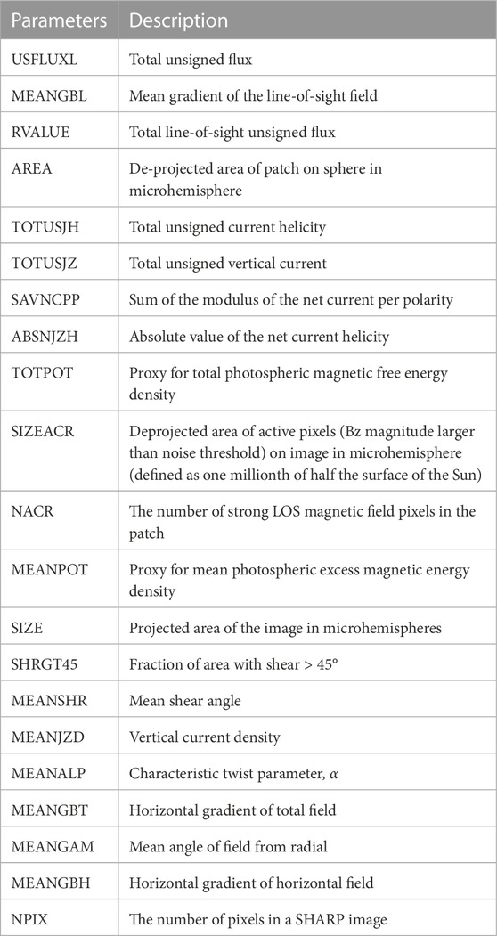
TABLE A3. List of SHARP parameters and brief descriptions.
Keywords: solar flare prediction, polar fields, solar cycle, mixture modeling, active regions
Citation: Aktukmak M, Sun Z, Bobra M, Gombosi T, Manchester IV WB, Chen Y and Hero A (2022) Incorporating polar field data for improved solar flare prediction. Front. Astron. Space Sci. 9:1040107. doi: 10.3389/fspas.2022.1040107
Received: 08 September 2022; Accepted: 29 November 2022;
Published: 21 December 2022.
Edited by:
Robertus Erdelyi, The University of Sheffield, United KingdomReviewed by:
Duncan Mackay, University of St Andrews, United KingdomHuw Morgan, Aberystwyth University, United Kingdom
Copyright © 2022 Aktukmak, Sun, Bobra, Gombosi, Manchester IV, Chen and Hero. This is an open-access article distributed under the terms of the Creative Commons Attribution License (CC BY). The use, distribution or reproduction in other forums is permitted, provided the original author(s) and the copyright owner(s) are credited and that the original publication in this journal is cited, in accordance with accepted academic practice. No use, distribution or reproduction is permitted which does not comply with these terms.
*Correspondence: Alfred Hero, aGVyb0B1bWljaC5lZHU=