 Paolo Massa
 A. Gordon Emslie
- Department of Physics and Astronomy, Western Kentucky University, Bowling Green, KY, United States
In this “Methods” paper, we investigate how to compress SDO/AIA data by transforming the AIA source maps into the Fourier domain at a limited set of spatial frequency points. Specifically, we show that compression factors of one order of magnitude or more can be achieved without significant loss of information. The exploration of data compression techniques is motivated by our plan to train Neural Networks on AIA data to identify features that lead to a solar flare. Because the data is spatially resolved and polychromatic (as opposed to spatially-integrated, such as GOES, or monochromatic, such as magnetograms), the network can be trained to recognize features representing changes in plasma properties (e.g., temperature, density), in addition to temporal changes revealed by Sun-integrated data or physical restructuring revealed by monochromatic spatially-resolved data. However, given the immense size of a suitable training set of SDO/AIA data (more than 1011 pixels, requiring more than one TB of memory), some form of data compression scheme is highly desirable and, in this paper, we propose a Fourier based one. Numerical experiments show that, not only Fourier maps retain more information on the original AIA images compared to straightforward binning of spatial pixels, but also that certain types of changes in source structure (e.g., thinning or thickening of an elongated filamentary structure) may be equally, if not more, recognizable in the spatial frequency domain. We conclude by describing a program of work designed to exploit the use of spatial Fourier transform maps to identify features in four-dimensional data hypercubes containing spatial, spectral, and temporal information of the state of the solar plasma prior to possible flaring activity.
1 Introduction
After more than a century and a half of ground-based optical observations of solar flares (Carrington, 1859; Hodgson, 1859), nearly a century of ground-based radio observations (Reber, 1944), and more than 70 years of study in wavelengths that can only be observed from spacecraft platforms (Tousey et al., 1951), our ability to forecast if and when these enigmatic events will occur, and to predict the likely nature of those events that do occur (e.g., electromagnetic radiation signatures; energy spectrum and elemental composition of energetic particles that are released into interplanetary space; extent, mass, and energy of the associated coronal mass ejection), is still at a fairly rudimentary level. It is generally understood (e.g., Tandberg-Hanssen and Emslie, 1988; Forbes et al., 2006) that flares, and their associated solar eruptive events, occur when energy stored in stressed, current-carrying magnetic fields in a solar active region (AR) is released—on timescales that are, perplexingly, orders of magnitude shorter than would be expected from global electrodynamic considerations. However, how magnetic energy is allowed to steadily build up in active regions over hours to days, without significant dissipation, only for a large fraction of this stored energy to suddenly be released on timescales of seconds to tens of minutes, is not well understood at all.
Prior to the occurrence of a flare, we can expect two main types of changes in the physical conditions in an active region.
• Morphological. It is well known, since the seminal studies of Hagyard et al. (1984a,b), that solar flares occur in regions of enhanced magnetic shear; this shear is a critical element in enabling magnetic field lines to reconnect (see, e.g., Priest and Forbes, 2007) and so release their stored magnetic energy as a flare and/or coronal mass ejection (CME). Quantitative measures of magnetic shear (i.e., deviation from a current-free potential magnetic field configuration) have been developed for a variety of complex magnetic field geometries (Falconer et al., 2008), as observed by solar magnetogram instruments, which can measure both line-of-sight field intensities (e.g., the Michelson Doppler Imager (MDI) on the NASA Solar and Heliophysics Observatory (SoHO); Scherrer et al., 1995) or, of considerably greater scientific value, vector magnetic field components determined from interpretation of the Stokes polarization parameters in suitbale spectral lines (e.g., Balasubramaniam and West, 1991). Such measures of magnetic complexity (including twist alone, and twist in concert with its longitudinal extent; Falconer, 1997) and/or magnetic field intensity (Falconer et al., 2006)) have been used to forecast coronal mass ejections from line-of-sight magnetogram observations (Falconer et al., 2002, 2007). In addition to large-scale morphological changes, it is also likely, in view of the need for the formation of small-scale regions (e.g., Drake et al., 2013) to efficiently dissipate magnetic energy, that the degree of filamentation of AR features (e.g., the striation of elongated structures into finer scales) may presage flaring activity.
• Thermodynamic. The release of magnetic energy will cause heating and the acceleration of non–thermal particles (see, e.g., Zharkova et al., 2011; Petrosian, 2016). The ensuing temperature and pressure gradients will drive changes in the atmospheric temperature and density profiles (see, e.g., Mariska et al., 1989), which are manifested in the intensities of emission in different spectral lines, notably in the ultraviolet and X-ray ranges of the spectrum (Mrozek et al., 2007). Thus, either independent of, or in concert with, morphological changes, we can expect significant changes in the emissivity in defined wavelength bands in the minutes leading up to the impulsive phase of a solar flare.
In summary, both morphological and thermodynamic changes can be expected to reveal important clues as to the likelihood of imminent flaring activity. As discussed in Section 2.3 below, the high-spatial-resolution, multi-wavelength observations of ARs made possible by the Atmospheric Imaging Assembly (AIA; Lemen et al., 2012) on the NASA Solar Dynamics Observatory (SDO) make them especially suitable for both types of measurement.
The ability to effectively forecast solar flares has two main benefits—operational and scientific. On the operational level, an empirical ability to predict flares (even without a deep understanding of the underlying causes) would in and of itself be valuable, inasmuch as it would allow prediction, and hence some degree of mitigation, of space weather events (Baker, 1998; Camporeale et al., 2018) that can occur when the flaring region is magnetically well-connected to the Earth. The recently-enacted Promoting Research and Observations of Space Weather to Improve the Forecasting of Tomorrow (PROSWIFT) legislation in the United States calls on federal research agencies such as NASA and NSF to work collaboratively with academia and public stakeholders, both public and private, to develop reliable flare prediction and mitigation strategies in order to protect several key elements of modern infrastructure, including satellite communications networks and electric power grids. Reliable flare predictions on timescales of hours to days can be used to warn of impending space weather events (or even to issue “all clear” forecasts for periods during which no significant space weather event is anticipated). From a scientific perspective, the ability to accurately predict flares requires (similar to the accurate prediction of terrestrial weather) a thorough understanding of the mechanisms through which flare energy is stored and released, and such an understanding would not only be of fundamental value to solar physics, but would also be applicable to many other areas of astrophysical research. Finally, in an intriguing blend of operational need and scientific investigation, the ability to make predictions of impending flare activity of timescales of minutes to tens of minutes can be used to inform the launch of short-duration rocket science payloads (e.g., Savage et al., 2021) that aim to “catch” a flare in its early stages, or to command the pointing of spacecraft instruments toward the Sun or a pertinent active region.
In this “Methods” paper, we present a plan to use machine learning models to identify features that presage a solar flare, using images acquired by the SDO Atmospheric Imaging Assembly. Distinct from other contemporary approaches that are based either on extracting features from solar images and using them for training Neural Networks (NNs; see e.g., Bobra et al., 2014; Georgoulis et al., 2021), or on feeding the networks with the images themselves (see Guastavino et al., 2022, and references therein), our methodology searches for patterns in the AIA images that are evident at different scales, as evidenced in spatial Fourier transforms of the native data. Fourier-based imaging algorithms are already in common use in interferometric radio astronomy, where each telescope-telescope baseline yields a corresponding spatial Fourier component of the source, and have also been used in hard X-ray imaging spectroscopy, providing much of the basis for the proposed methodology (see Section 3).
The motivation behind the use of spatial Fourier transform information for feature identification and extraction is twofold. First, potential approaches that are based on training NNs directly on AIA images are very demanding from a computational point of view, both in terms of memory needed for storing such a large amount of data and in terms of the computational power needed for processing it. Standard SDO/AIA images are 4,096 × 4,096 pixels and, even if cropped around an AR area of interest (say, 200 × 200 pixels), a training set consisting of 10,000 “datacubes,” each involving 20 min of data (100 observing intervals at the highest—12 s—time cadence), and using all seven AIA EUV channels, would contain 10, 000 × 100 × 200 × 200 × 7 ≃ 3 × 1011 pixels. Assuming 4 bytes per pixel, the resulting data set would be more than one TB, far too large to be easily stored and processed. Some degree of data compression is therefore highly desirable. Second, certain types of features (such as spatial periodic effects) are more discernible in the Fourier domain, so that analysis of spatial Fourier components may offer further insight into the nature of the features that lead to a flare.
To the best of our knowledge, there have been no previous attempts to address the flare forecasting task using spatial Fourier components as primary data for training NNs. However, it is known in the machine learning literature (Xu et al., 2020) that data compression without significant loss of information can be more easily achieved in the frequency domain, since many spatial frequencies are simply not relevant for tasks addressed by NNs. Moreover, several recent studies have demonstrated that NN performance and training efficiency can indeed be improved if the networks are provided with input data that has been transformed into the frequency domain (e.g., Hertel et al., 2016; Xu et al., 2020; Zhang et al., 2020). These results lend considerable encouragement to the idea of flare forecasting utilizing “visibility” maps corresponding to the AIA images instead of the images themselves.
Our approach is inspired by indirect Fourier imaging techniques that have been applied to hard X-ray imaging spectroscopy data from instruments such as the Reuven Ramaty High Energy Solar Spectroscopic Imager (RHESSI; Lin et al., 2002) and the Spectrometer/Telescope for Imaging X-rays (STIX; Krucker et al., 2020) on board the Solar Orbiter mission. For these bi-grid collimator instruments, the native form of the data is a sparse set (30 for STIX and up to an order of magnitude more for RHESSI) of spatial Fourier components, termed “visibilities.” This fundamental nature of the RHESSI and STIX data therefore required the development and implementation (Piana et al., 2022) of image reconstruction algorithms based on such sparsely-populated spatial frequency information, with, as it turned out, considerable success. Thus, although the native form of the SDO/AIA data is, of course, a set of conventional pixel-by-pixel maps, it is still of interest to explore converting this information into Fourier component form, with a view to training NNs on such highly-compressed, informationally-dense, data sets. We shall show below that much of the useful information in an AIA image can indeed be encapsulated in a relatively small number of sparsely-distributed spatial Fourier components.
The outline of the paper is as follows. Section 2 is devoted to the description of the AIA data under consideration, and its potential to reveal properties of solar ARs that presage a solar flare. In Section 3 we present our spatial-Fourier-transform approach to feature identification from the AIA data and we show how to create data hypercubes that contain, in a dataset of manageable size, essential information on the spatial, temporal, and temperature structure of pre-flare ARs. Application of this method to sample AIA data is presented in Section 4, and the results discussed in Section 5. Finally, our conclusions are presented in Section 6.
2 The potential of different data sets for flare forecasting
2.1 GOES soft X-ray flux
The likelihood of imminent flaring activity can be ascertained by monitoring changes in the emission in the 1–8 Å soft X-ray channel of the Geostationary Operational Environmental Satellites (GOES; Nagem et al., 2018; Ehrengruber and Melchior, 2020). However, while changes in the thermodynamic properties of the solar corona during pre-flare activity do produce excess emission in the GOES 1–8 Å channel, such measurements suffer from four main drawbacks as a reliable diagnostic of imminent flaring activity:
• precursor soft X-ray emission takes place in an AR that may have a substantially enhanced level of soft X-ray emission already, so that the contrast in the pre-flare region is relatively low;
• soft X-ray emission comes from heated ten-million-degree material, and so the emission in this waveband becomes substantial only after a significant amount of flare energy has already been released;
• GOES measures soft X-ray emission from the entire solar disk, and hence is not especially sensitive to strong local enhancements, such as those that may precede a flare; and
• soft X-ray emission is dominated by broadband continuum emission, which, although a valid indicator of energy release, is not the best diagnostic of detailed information about the evolving temperature structure of the solar atmosphere.
All of these factors imply that, while a rise in the GOES flux may well portend a subsequent flare event, it need not necessarily do so. Moreover, useful signals may well be swamped by soft X-ray emission unrelated to the flare development and, since the signal is integrated over the entire solar disk, information on the location of the impending flare would not be immediately available. This could be a major drawback in an operational context, such as observing campaigns (e.g., Savage et al., 2021) involving instruments with a limited field of view that need to be pointed toward the correct AR in order to observe the resulting flare.
2.2 Magnetograms
Given the key role that the solar magnetic field plays in storing and releasing the energy of a flare, a clearly appropriate, and also more surgical, approach to flare forecasting relies on the use of line-of-sight magnetograms, such as those recorded by the Helioseismic and Magnetic Imager (HMI; Scherrer et al., 2012) on board the SDO. Prominent features in ARs that have configurations that are believed to lead to subsequent flaring (e.g., regions of high magnetic shear; Moore et al., 2001) are extracted and machine learning models are trained on these features to predict the occurrence of a flare several (e.g., 12, 24, 48) hours in advance. There are at least two sets of features that are derived from HMI magnetograms: first, features contained in the metadata of the Spaceweather HMI Active Region Patch (SHARP) data products (Bobra et al., 2014) and, second, features defined within the FLARECAST project (Georgoulis et al., 2021). Both sets of features have been proven to contain information related to flare occurrence, and several works (e.g., Bobra and Couvidat, 2015; Liu et al., 2017; Florios et al., 2018; Campi et al., 2019) have assessed the predictive capabilities of machine learning methods trained on those sets. More recently, approaches based on training Convolutional Neural Networks (CNNs) directly on HMI magnetograms (or on time sequences of HMI magnetograms) have been investigated (see e.g., Huang et al., 2018; Li et al., 2020; Yi et al., 2021; Chen et al., 2022; Guastavino et al., 2022).
2.3 SDO/AIA data
An even more surgical approach to flare prediction is suggested by the availability of high-spatial-resolution, multi-wavelength, EUV observations obtained with the SDO/AIA telescope, which has provided (along with other data) full–disk 4,096 × 4,096 pixel images of the Sun, with 0″.6 × 0″.6 resolution, in seven different EUV wavelengths (93 Å, 131 Å, 171 Å, 193 Å, 211 Å, 304 Å, 335 Å) every 12 s since its launch in 2012; this represents an unprecedented archive resource for the investigation of the physical processes that lead to the onset of a solar flare. Due to the immense amount of data available, and an open policy for data distribution, this archive has attracted a lot of attention in the past few years for the development of machine learning methods (e.g., Huang et al., 2018; Galvez et al., 2019; Inceoglu et al., 2022). Although several recent works have dealt with combining HMI and AIA data for improving the predicting capabilities of machine learning techniques (e.g., Jonas et al., 2018; Nishizuka et al., 2018), to the best of our knowledge, no attempt has been made to forecast solar flares by using information encoded in the AIA data alone.
By contrast with the broadband emission in the GOES 1–8 Å band, extreme ultraviolet (EUV) emission, produced in the 105–107 K solar atmosphere, including the high and low corona and the so-called “transition region” between the hot corona and the relatively cool (∼ 104 K) solar chromosphere, is characterized by a set of intense, relatively narrow, emission spectrum lines, each produced by a given atomic species that is formed over a fairly narrow range in temperature T. The intensity (erg cm−2 s−1) observed at a distance R = 1 AU in a given image pixel of area A (cm2) and observing channel i is proportional to the integral of the line-of-sight-integrated Differential Emission Measure (DEM; cm−5 K−1; see, e.g., Phillips et al., 2008) in that pixel multiplied by an emissivity function Gi(T) (erg cm3 s−1) which accounts for a variety of effects, including the abundance of the responsible atomic species and its ionization and excitation states. Formally, the intensity in a given pixel (x, y) in the ith AIA channel at time t is given by
Changes in the plasma properties of the solar atmosphere (e.g., heating, cooling, mass motions) during a magnetic reconnection event can cause very significant changes in both density and temperature profiles, with corresponding changes in the differential emission measure profile DEM(x, y; T; t) and hence in the observed intensities Ii(x, y; t). Cheung et al. (2015) have shown how the integral Equation 1 may be inverted to construct the emission measure profile DEM(x, y; T; t) at each AIA pixel (x, y) and time t, given the time evolution of the observed intensities Ii(x, y; t). Such data hypercubes DEM(x, y; T; t) contain information on the spatial, thermal, and temporal evolution of the plasma. They can reveal much more information than monochromatic HMI data: both can identify physical restructuring of features in the field of view, but the AIA data hypercubes can also show changes in the DEM profiles within a source of interest; changes that can reveal heating and cooling processes, either in the absence of, or coupled with, physical restructuring.
Figure 1 shows two 200-pixel × 200-pixel (120″ × 120″) images, recorded in the 304 Å (panel (A)) and 131 Å (panel (B)) AIA channels on 26 October 2014 at 12:48:17 UT and 12:48:20 UT, respectively. The images show AR 12192 a few minutes before it produced a C9.2 GOES class flare extending from 13:04 UT and 13:16 UT. In an attempt to reproduce the essential features of these images with fewer data points, Figure 2 shows these “ground-truth” images binned into both 10-pixel by 10-pixel, and 5-pixel by 5-pixel blocks, resulting in images with 20 × 20, and 40 × 40 data points, respectively. Although the amount of data required to produce these images is considerably less (factors of 100, and 25, respectively) than for the original images, there is clearly a significant loss of information in the spatially-binned images. On the other hand, as we shall show below, compressing the data using spatial Fourier transforms still produces a much smaller dataset, with a size comparable to that used to construct Figure 2, but retains essential information on the features in the source maps.
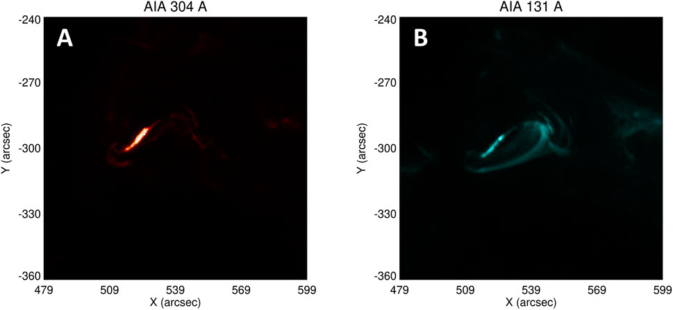
FIGURE 1. Images taken in the 304 Å (A) and 131 Å (B) SDO/AIA channels on 2014 October 26 around 12:48 UT. The images have the standard
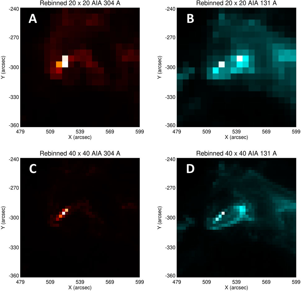
FIGURE 2. The images of Figure 1, binned into “blocks” measuring 10-pixels by 10-pixels (panels (A) and (B) and 5-pixels by 5-pixels (panels (C) and (D)). Panels (A) and (B) each contain 20 × 20 = 400 data points, while panels (C) and (D) each contain 40 × 40 = 1,600 data points. Note the significantly degraded information content in these images compared to the 40,000-data-point images of Figure 1.
3 Visibilities: Sparsely-populated spatial Fourier transforms of a map
The formal relationship between an image I (x, y) and its spatial Fourier transform
where (xo, yo) is a suitably chosen reference point; it corresponds to the point of zero phase in the image, and is usually chosen near the region of brightest intensity, to avoid unnecessary phase oscillations in the brightest regions of the source that contribute most to the integral in Eq. 2. The standard Fast Fourier Transform (FFT) algorithm generates amplitudes and phases of spatial Fourier components at a number of spatial frequency (u, v) points that is equal to the number of pixels in the original image, and hence results in little to no data compression. However, as we shall show below, it is not necessary to evaluate each and every spatial Fourier component in order to obtain essential information on the features present in a typical pre-flare AIA image; much of the useful information in an image can be encapsulated in a relatively small number of sparsely-distributed spatial Fourier components (or “visibilities”). Use of such a sparse set of Fourier components permits not only a considerable degree of data compression, but also the intriguing opportunity to identify features that would not necessarily be immediately obvious from spatial maps (e.g., striation of a filament into longitudinal sub-filaments). Such a data compression scheme is commonly used in image compression formats such as. png, but its application to analysis of solar data, in particular with application to flare prediction, is, to the best of our knowledge, new.
Solar hard X-ray images over the last 2 decades have been obtained through the use of bi-grid collimator instruments such as RHESSI (Lin et al., 2002) and STIX (Krucker et al., 2020). As explained in Hurford et al. (2002) and Piana et al. (2022), the native data product of such instruments are spatial Fourier transforms of the image, with the wavevector (u, v) components reflecting the pitch (inversely proportional to
Figure 3 illustrates the capability of computed visibilities to yield essential information on source structure, using synthetic maps containing single elliptical Gaussian sources with varying eccentricity, starting with a zero-eccentricity (circular) Gaussian (panels (A1-A4)). For the circular Gaussian source, the Fourier transform (visibility) amplitude map is, of course, another Gaussian, with a width in the spatial frequency domain that is inversely proportional to the width of the spatial Gaussian source. As the eccentricity increases, the characteristic scale associated with the minor axis decreases, so that the spatial Fourier transforms of the source maps (computed using the FFT algorithm; panels (B1-B4)) extend to higher and higher spatial frequencies, with the orientation of the line from the origin in the spatial frequency plane to the region of high Fourier power being oriented parallel to the minor axis (i.e., perpendicular to the major axis) of the spatial ellipse. Panels (C1-C4) in Figure 3 show the spatial Fourier transform (visibility) amplitudes computed using the sparse set of (u, v) points shown in panel (B) of Figure 4. We have verified that the apparent distortion of the expected elliptical Gaussian shape is entirely due to the manner in which the sampled (u, v) values, plotted as a uniformly-spaced pattern here, are actually unevenly distributed in the (u, v) plane in accordance with the “square-root” grid of Figure 4; furthermore, the calculated visibility amplitudes on the relatively coarse grid of spatial frequency (u, v) values sampled match those obtained on the finer grid used by the FFT.
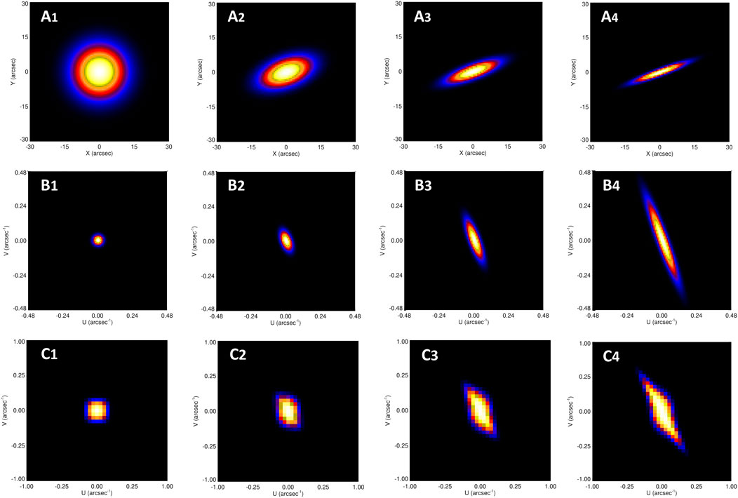
FIGURE 3. (A1––A4) A series of idealized elliptical Gaussian sources with different eccentricities, starting with a zero-eccentricity (circular) Gaussian. (B1–B4) Amplitudes of the spatial Fourier transforms (“visibilities”) of these sources, calculated using the FFT algorithm. (C1–C4) Visibility amplitudes obtained using the discrete Fourier transform 2, considering a relatively small (39 × 39) number of spatial frequency points selected in accordance with panel (B) of Figure 4. Note that the FFT-generated transforms in panels (B1–B4) are generated at spatial frequency points that have equal spacing in both u and v, whereas panels (C1–C4) use a grid with equal spacing in
Although the native form of the RHESSI and STIX data was such a sparsely-distributed set of visibilities, the high-quality pixel-by-pixel images of the AIA dataset do not, of course, compel us to examine images in the spatial Fourier domain. But our experience with the RHESSI and STIX datasets show that it nevertheless may be advantageous to do so anyway. First of all, it allows us to compress a considerable quantity of data into a relatively small number of Fourier components without significant loss of information, as proved by the results obtained by means of many algorithms which have been developed for solving visibility-based image reconstruction problems (see Massa et al., 2022; Piana et al., 2022). This is useful in significantly reducing the computational time and effort needed to train NNs for analyzing datacubes with high data content. But there is another possible advantage to a shift to the spatial frequency domain: as we shall show below, it also allows ready identification of features that might otherwise escape recognition. Since each visibility
We now discuss the range of spatial frequencies necessary to provide adequate coverage of the range of spatial scales present in the images of Figure 1. At one extreme, spatial frequencies |u| must be sampled up to a value corresponding to the physical scale of an image pixel, viz. 0.6″; using the standard Cauchy-Schwartz “uncertainty principle” inequality Δu Δx ≳ 1/2, this requires that we sample up to values of |u| at least as large as 1/(2 × 0.6) ≃ 0.8 arcsec−1. We have therefore chosen |umax| = |vmax| = 1 arcsec−1, so as not to over-resolve fine features on the scale of individual pixels. At the other extreme, the maximum value of |x| in the images is 60″, corresponding to |u| = 1/(2 × 60) ≃ 0.08 arcsec−1; accordingly, we choose |umin| = |vmin| = 0.01 arcsec−1. The range of sampled |u| values thus spans a range of 100:1, equal to the ratio of the maximum value |x| to the pixel size. Between 0.01 and one arcsec−1, we selected |u| and |v| values that are equally spaced in
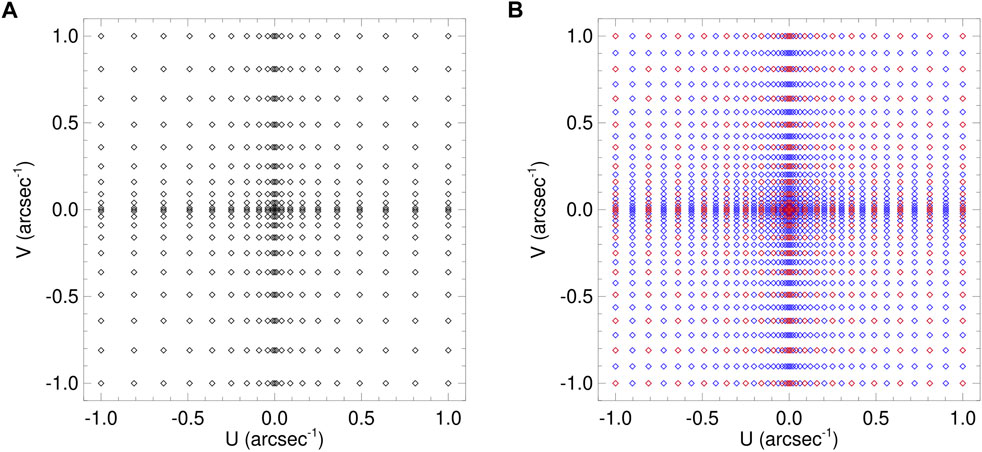
FIGURE 4. Spatial frequency points at which visibility information is computed. Two sets of sampled points are shown. (A) A relatively coarse 21 × 21 grid; (B) a finer 39 × 39 grid. In panel (B) we plot the 39 × 39 grid in blue and, for comparison, we overlay the 21 × 21 grid in red.
Figure 4 shows two such samplings of the spatial frequency (u, v) space. Panel (A) shows a relatively coarse 21 × 21 point grid, corresponding to the sampled values [0, 0.1, 0.2, … , 0.9, 1.0] of
Given a finite set of visibilities
where (Δu Δv)i,j is the area in the (u, v) plane represented in the Riemann sum by the value
4 Application to AIA images
Figure 5 shows the visibility amplitude maps constructed using sets of 21 × 21 (panels (A) and (B)) and 39 × 39 (panels (C) and (D) spatial frequencies (u, v), distributed as shown in Figure 4. Eq. 2 shows that the visibility
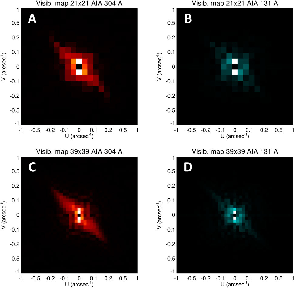
FIGURE 5. Spatial Fourier transform (“visibility”) amplitude maps of the images in Figure 1, using Eq. 2 applied at the spatial frequency (u, v) points shown in both panels of Figure 4. Panels (A) and (B) contain 21 × 21 points, while panels (C) and (D) contain 39 × 39 points, respectively.
Panels (A) and (B) of Figure 6 show the original SDO/AIA 304 Å and 131 Å images of Figure 1. Panels (C) through (F) show images reconstructed from the visibility maps of Figure 5 (including the associated phases, where the point (xo = 539, yo = −300) was chosen as the phase origin). The reconstructions were performed using the MEM_GE method (Massa et al., 2020), which has already been applied with considerable success in the rendition of RHESSI and STIX images. This algorithm minimizes the χ2 discrepancy between the observed visibilities and those predicted from the reconstructed image, subject to a regularization constraint involving the magnitude of a suitably-defined entropy function. As described by Massa et al. (2020) and Piana et al. (2022), the method significantly reduces the “ringing” effects (which appear in this case as a periodic repetition of the main feature, oriented approximately along a direction corresponding to the longitudinal axis of the principal source—see, for example, panel (J) of Figure 6) by imposing a smoothness constraint to the solution. Although “ringing” artifacts are still present in the MEM_GE reconstructed image, their intensity is much less pronounced compared to what they would be if the image had been reconstructed through a direct inverse Fourier transform (Eq. (3)). The reconstructions in panels (C) and (D) were performed using the 21 × 21 grid of sampled (u, v) points (panel (A) of Figure 4), while the reconstructions in panels (E) and (F) were performed using the 39 × 39 grid (panel (B) of Figure 4).
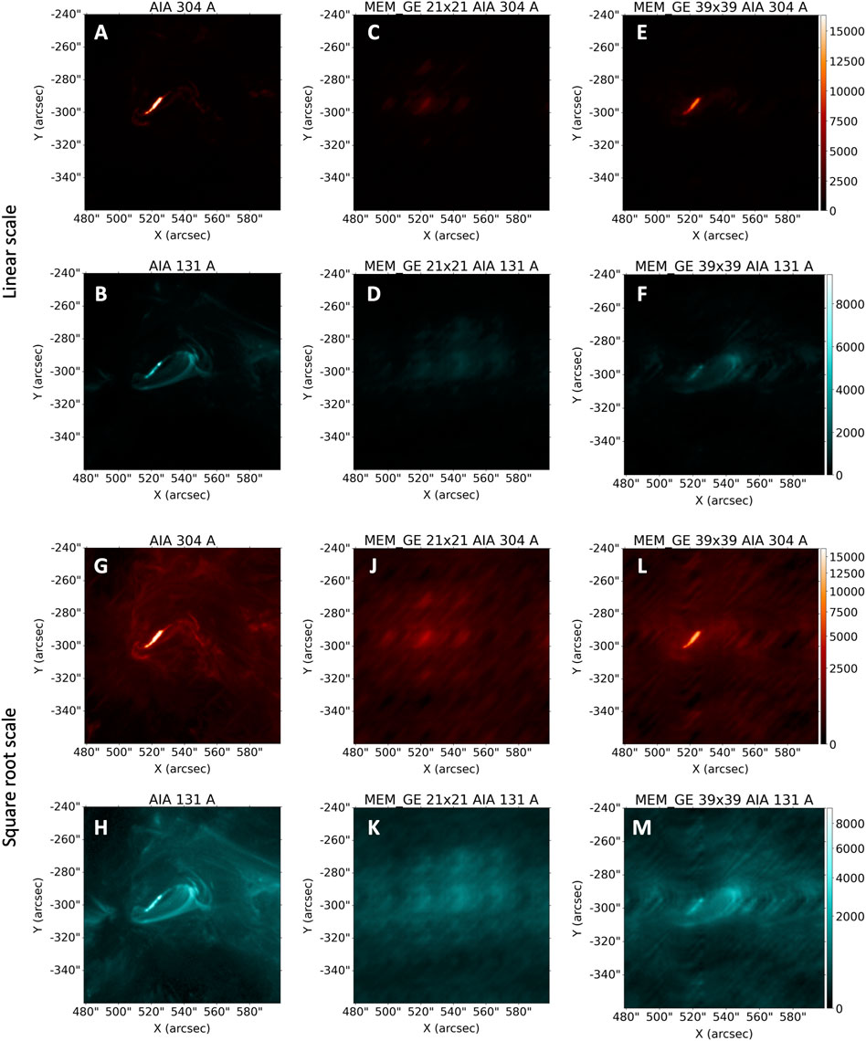
FIGURE 6. Reconstructed images using the visibility maps of Figure 5 (including the associated phases, see text for details) and the MEM_GE algorithm. (A and B) original images; (C and D) reconstructed images using 21 × 21 visibility points (panel (A) of Figure 4); (E and F) reconstructed images using 39 × 39 visibility points (panel (B) of Figure 4). (G–M) show the same information, with a square root intensity scaling applied to provide greater detail on relatively weak pixels. The color map is shared by panels in the same row.
Panels (G) through (M) show the same information as panels (A) through (F), but using a square-root-scaled color table in order to highlight pixels with weaker intensity. Panels (J) and (K), both of which were reconstructed using the relatively coarse 21 × 21 grid of sampled (u, v) points, reveal four rather obvious “ghost” sources, located at positions Δx ≃ 25″ above/below and left/right of the actual principal source. Such a displacement corresponds to a spatial frequency u = 1/(2Δx) ≃ 0.02 arcsec−1, showing that the region of the (u, v) plane around this value is not adequately sampled by the 21 × 21 grid. Indeed, this value of u corresponds to
To evaluate the reliability of the MEM_GE reconstructions, and hence to show that visibility maps do indeed retain essential information about the original AIA images, we can compare the pixel values of the reconstructed images to those of the ground-truth maps. Figure 7 shows two-dimensional histograms of the pixel values of the MEM_GE reconstructions (ordinate) plotted as a function of the corresponding pixel values (abscissa) in the original AIA images. Since the dynamic range of the AIA maps is rather large, and there are only a few very intense pixels, we applied a logarithmic binning to both the x- and y-axes of each histogram, which are plotted with respect to logarithmic axes. The color scale shows the number of points that belong to each (AIA intensity, reconstructed intensity) bin.
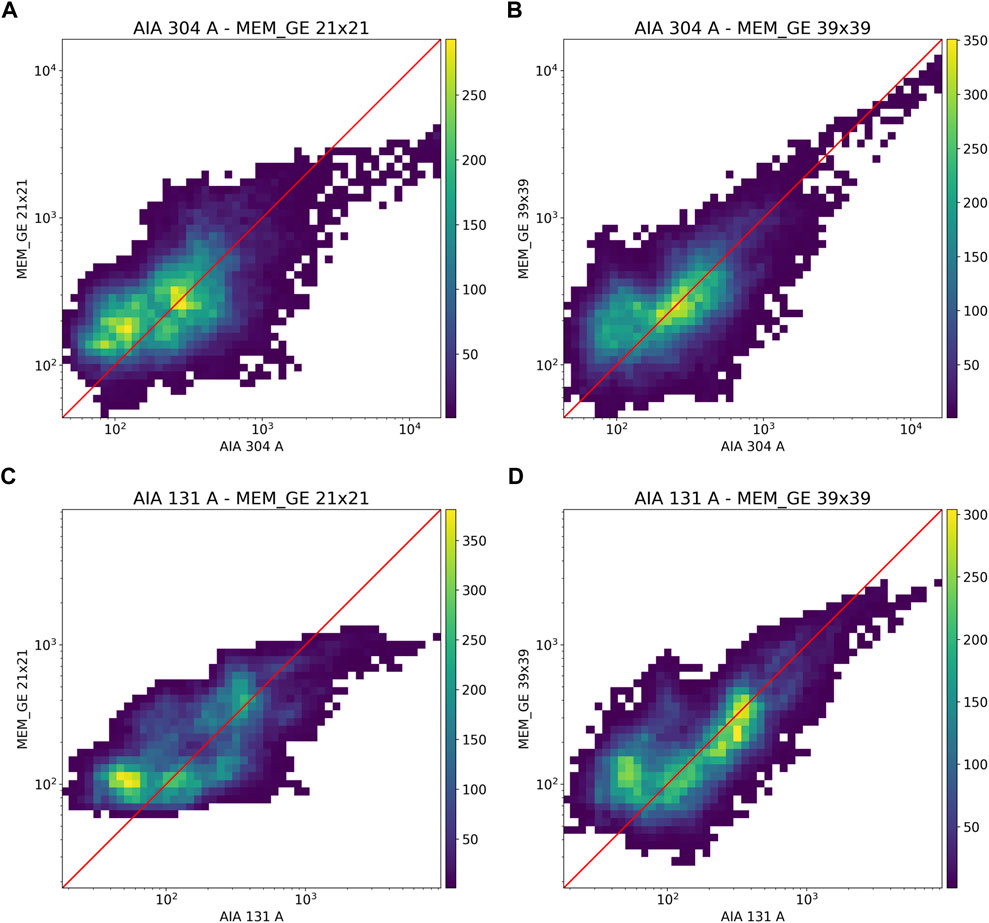
FIGURE 7. Histograms of the pixel values of the MEM_GE reconstructions, shown in Figure 6, plotted (vertical axes) versus the corresponding pixel values in the AIA maps (horizontal axes). Both the x- and y-axes have been binned in logarithmic steps and the color map refers to the number of points falling within each bin. Panels (A) and (B) show the histograms of the MEM_GE reconstructions of the AIA 304 Å image from 21 × 21 and from 39 × 39 visibilities, respectively. Panels (C) and (D) show the same information, but for the AIA 131 Å image. In each panel, a logarithmic scaling is applied to both the x- and y-axes and a red line representing equality is plotted as a reference.
Panels (A) and (C) of Figure 7 shows that MEM_GE, when used with the limited (21 × 21) number of visibilities corresponding to the (u, v) points in the left panel of Figure 4, generally fails to reproduce the original AIA images with high fidelity. The MEM_GE reconstructions generally underestimate the intensities in bright pixels, while overestimating the intensities of weaker pixels (e.g., the yellow areas above the red line that represents equality of the original and reconstructed pixel intensities). This is due to an insufficient sampling of the (u, v)-plane: the resulting “ringing” effects in the reconstructions smear out the information in low and high pixel values (as shown also in Figure 6, panels (C), (D), (J), and (K)), resulting in a smaller dynamic range than in the original images, as evidenced by the fact that the “symmetry axis” of the 2-D histogram shapes lies at an angle less than 45° to the horizontal axis. However, panels (B) and (D) of Figure 7 demonstrate that sampling the set of 39 × 39 visibilities (right panel of Figure 4) significantly increases the accuracy in the reconstruction, consistent with what was shown in panels (E), (F), (L), and (M) of Figure 6. In those histograms, a much larger number of points is concentrated around the red 45° identity line, although the MEM_GE reconstructions still tend to slightly underestimate the peak values in the AIA images.
To compare the loss of information associated with Fourier–based data compression with that of straightforward binning of spatial pixels, we quantitatively evaluated the differences between the original AIA images and the images formed by MEM_GE reconstructions, and spatial rebinning, respectively. We considered different values for the data compression factor, defined as DCF = (200/N)2, where N2 is either the number of spatial Fourier component values used (because of the Fourier transform antisymmetry with respect to the origin of the (u, v)-plane, these N2 values are N2/2 amplitudes and N2/2 phases) or the number of original pixels binned into each “metapixel, \dprime respectively. We used three metrics: (1) the mean Structural SIMilarity index (SSIM, Wang et al., 2004), which compares4 intensities, contrast and structure of the original and reconstructed images; (2) the Normalized Root Mean Squared Error (NRMSE), a dimensionless metric that measures the pixel-averaged RMS difference between the original and reconstructed images, expressed as a fraction of the mean pixel intensity; and (3) the Peak Signal to Noise Ratio (PSNR), which is the ratio of the intensity of the brightest pixel to the (un-normalized) root mean square error (RMSE), expressed in decibel (dB) units, such that PSNR = 20 log10(Imax/RMSE). We note that for the PSNR and SSIM metrics, a larger number represents a better agreement (in particular, a 1.0 value for SSIM represents a perfect match), while for the NRMSE metric, a smaller number represents a better fit. Thus, the y axis of the NRMSE plot is reversed.
Panels (A) through (C) of Figure 8 show the values of these three metrics, for the AIA 304 Å image, as a function of the data compression factor. Since each of the metric evaluations used require images with the same number of data points, we replicated each pixel of the rebinned images to create a 200/N × 200/N square of identically-valued pixels at each location, so that the final map size is again 200 × 200 (but the compression effect remains unaltered). Panels (D) through (F) of Figure 8 show the values of the same three metrics for the AIA 131 Å image.
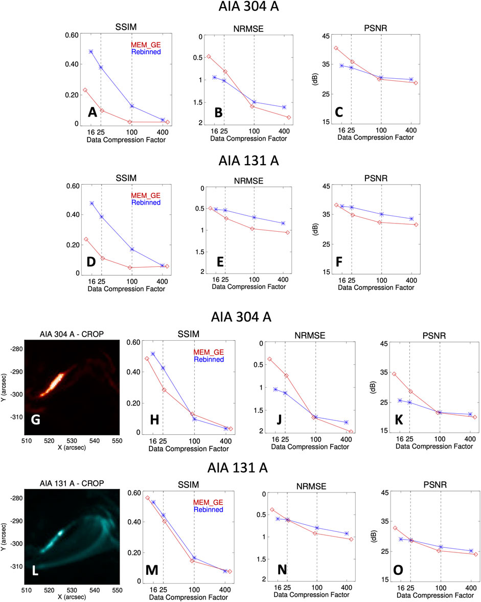
FIGURE 8. SSIM, NRMSE, and PSNR metrics associated with the MEM_GE reconstructions (red) and the spatially rebinned images (blue) for different data compression factors. Panels (A) through (C) show the metrics for the AIA 304 Å image shown in Figure 1, while panels (D) through (F) show the same information for the AIA 131 Å image. Panels (H) through (K), and (M) through (O), are analogous to Panels (A) through (C), and (D) through (F), respectively. However, in this case, the metrics are computed with respect to a cropped 70-pixel × 70-pixel subregion of the original images, as shown in panels (G) and (L). A logarithmic scaling has been applied to the x-axis of each metrics panel; in addition, in order that “better” be represented by a point nearer the top of each panel, the y axes of panels (B), (E), (J), and (N), representing the NRMSE metric, have been reversed. The vertical lines at DCF ≃ 25 and 100 in each panel represent the data compression factors corresponding to the rebinned images shown in Figure 2. The DCF values adopted for the MEM_GE reconstructions are slightly different from those of the rebinned images, as shown by the small horizontal shifts between the red and blue points.
We first consider the AIA 304 Å results (Panels (A) through (C)). For high data compression factors DCF ≳ 100, the visibility-based MEM_GE reconstructions and spatially-rebinned images have comparable (and quite poor) values for all three metrics, showing that such a high level of data compression is simply not feasible using either method. As the DCF is reduced to more reasonable values, the SSIM metric shows an improvement of a factor of about 10 (from ≃ 0.05 to ≃ 0.5) for the spatially-rebinned compression method, and an slightly smaller factor of
By contrast, as the DCF is reduced, the RMSE and PSNR metrics for both methods improve, but now more markedly so for the visibility-based MEM_GE method. Quantitatively, on reducing the DCF from ≃ 400 to ≃ 16, the NRMSE for the spatially-rebinned images decreases by a factor of
Next considering the AIA 131 Å results (panels (D) through (F)), for high data compression factors the MEM_GE reconstruction method gives consistently poorer metrics than for the spatially-rebinned images, with NRMSE values about 1.3 times larger, and corresponding PSNR values about 2 dB lower. This poorer performance reflects the more complicated spatial structure in the 131 Å image, which renders an accurate reconstruction with a limited number of visibility values more challenging, especially when high data compression factors are involved. However, as the DCF is reduced, the metrics associated with the MEM_GE method improve by a more significant factor, resulting, by DCF ≃ 16, in NRMSE and PSNR values that are comparable to those for the spatial rebinning data compression method.
A possible reason for the apparent poor performance of the MEM_GE reconstructions when the SSIM metric is applied, is as follows. As shown in panels (E) and (F), and (L) and (M) of Figure 6, MEM_GE is able to retrieve with greatest accuracy the most intense parts of the AIA images, while the areas with lower-intensity pixels are significantly corrupted by the “ringing” artifacts caused by the limited number of Fourier components utilized. Hence, comparing MEM_GE image reconstructions of the entire map with the original AIA data includes a significant area in which these “ringing” artifacts are present and hence in an overall degraded representation of the performance of the method. This could lead to an apparent conclusion that Fourier-based data compression methods are less effective than straightforward rebinning of pixels in physical space.
However, it is important to point out, particularly for the purposes of flare forecasting, that it is generally only the brightest areas of the AIA images that are most likely to contain information about the underlying physical processes that lead to a flare. Recognizing this, in Panels (H) through (K) and (M) through (O) of Figure 8 we compare the methods using only a 70-pixel × 70-pixel subregion (Panels (G) and (L)) that is centered around the most intense features, and contains (200/70)2 ≃ 8× fewer pixels than the original 200-pixel × 200-pixel image.
Panels (H) and (M) show that the SSIM values for both methods, applied to both the 304Å and 131Å cropped images, are now almost identical, and they both show about a tenfold improvement with reduction in the DCF. For the 304 Å image, as the DCF is progressively reduced to lower values, the NRMSE (panel (J)) reduces by a factor of almost two for spatial rebinning, but by an even greater factor of five for MEM_GE. These improvements in the NRMSE correspond to PSNR improvements (panel (K)) of ≃ 6 dB and ≃ 14 dB, respectively. Thus, in comparing only the maps in the vicinity of the brightest pixels, the MEM_GE method significantly outperforms the spatially-rebinning method by about 10 dB PSNR (or, equivalently, produces an NRMSE that is a factor of 3 less) at more practicable data compression factors. For the 131 Å image, the SSIM metrics are again comparable for both methods, while the NRMSE (panel (N)) now improves from ≃ 1.0 at a DCF ≃ 400 to ≃ 0.6 (rebinning) and ≃ 0.4 (MEM_GE) at DCF ≃ 16. The PSNR (panel (O)) similarly varies from ≃25 dB at a DCF ≃ 400 to ≃ 29 dB (rebinning) and ≃ 33 dB (MEM_GE), respectively, at DCF ≃ 16.
We finally observe that, while reconstructing an image from the visibilities and comparing it to the original AIA map is one method of evaluating the effectiveness of the compression method, this test is potentially biased for at least two reasons. First, the results depend heavily on the reconstruction algorithm used. The MEM_GE algorithm used was initially developed to analyze sparse visibility data from the RHESSI and STIX instruments (Massa et al., 2020; Massa et al., 2022; Piana et al., 2022), the data from which are inherently spatial Fourier transforms corresponding to a pre-selected set of (u, v) points, chosen to address the science requirements of those missions (Hurford et al., 2002; Krucker et al., 2020). It is therefore distinctly possible that results shown in Figures 7, 8 could improve if a reconstruction method were used that was more tailored to the form of the AIA data. Second, once the number of Fourier components to be used for compressing AIA images (and hence the data compression factor) has been fixed, we still have the freedom to adjust the location of the sampled spatial frequencies in order to “capture” the maximum amount of information in the images themselves. The grids of (u, v)-points that we adopted, as shown in Figure 4, apparently do represent a reasonable choice, given their success in replicating features in the orginal image, but they are almost certainly not optimal. We refer the reader to Section 5 (and Figure 10) for a discussion about a machine learning technique that could be used for adapting the location of the (u, v)-frequencies to best represent AIA images for a given data compression factor.
Looking at the top left and (conjugate) bottom right quadrants of the panels in Figure 5, there is a rather obvious difference in intensity (i.e., Fourier spectral power) between the left (304 Å; panels (A) and (C)) and right (131 Å; panels (B) and (D)) sets of frames. In the 304 Å visibility amplitude maps, there is considerable spectral power along a region connecting the second and fourth quadrants, but such a feature is not as evident in the 131 Å visibility maps. The presence of such a feature in a visibility map corresponds (cf. Figure 3) to the presence of a source with a narrow width measured in a direction oriented parallel to the line joining the origin and the (u, v) region in question (in this case, top-left to bottom-right). Indeed, inspection of the original data of Figure 1 shows just such a bright narrow-width source in the 304 Å image, which is not as pronounced in the 131 Å image. We submit that this feature is just as evident, and possibly even more pronounced, in the visibility maps, even though these maps contain far fewer data points than in the original spatial maps.
We pursue this further in Figure 9. Panels (A) and (B) show SDO/AIA 304 Å AIA images taken 12 s apart, at 12:48:07 UT and 12:48:19 UT, respectively. There is a rather obvious brightening with time of a core region within the principal source, which is clearly revealed in panel (C), which is the difference map [(B)-(A)]. Panels (D) and (E) are the corresponding 39 × 39 visibility amplitude maps, and their difference [(E)-(D)] is shown in panel (F).
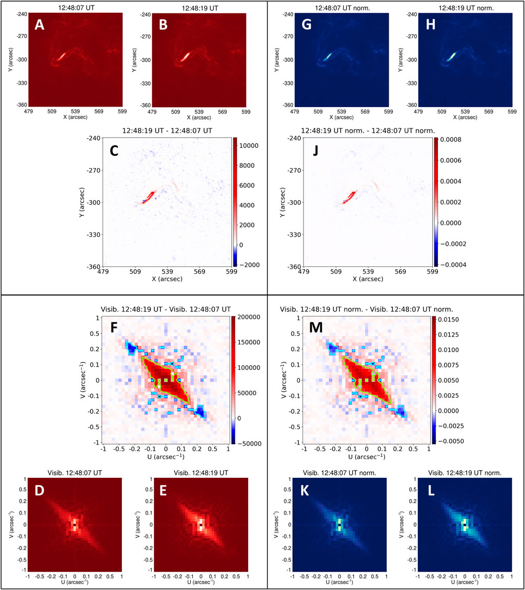
FIGURE 9. Top left quadrant: 304 Å images at 12:48:07 UT (A) and 12:48:19 UT (B), and their difference image [(B)–(A)] (panel (C)). Bottom left quadrant: Visibility amplitude maps (D) and (E) corresponding to maps (A) and (B), respectively, and their difference [(E)–(D)] (panel (F)). Top right quadrant: Normalized intensity maps (G) and (H), corresponding to images (A) and (B), respectively, and their difference [(H)–(G)] (panel (J)). Bottom right quadrant: Visibility amplitude maps (K) and (L) corresponding to the normalized intensity maps (G) and (H), respectively, and their difference [(L)–(K)] (panel (M)). Contour levels corresponding to 20% of the minimum (negative) value (light blue) and 33% of the maximum value (light green) are overlaid in each of the visibility difference maps (F) and (M). Specifically, the light blue contours correspond to values of − 9,900 (panel (F); un-normalized) and − 0.001 ((panel (M); normalized), while the light green contours correspond to values of 66,000 and 0.004, respectively.
The interpretation of visibility amplitude difference maps is rather subtle. Changes in visibility amplitude can result from two main effects: an overall change in the source brightness, and/or a restructuring of the source to different spatial scales. To emphasize the latter effect, panels (G) and (H) show normalized (to the total signal in the overall map) source maps corresponding to maps (A) and (B), and panels (K) and (L) show the corresponding visibility amplitude maps. Panel (J) shows the difference in the normalized spatial maps [(H)-(G)] and panel (M) shows the difference [(L)-(K)] in the normalized visibility maps.
Panel (M), showing the shift over time in the distribution of visibility amplitude over the spatial frequency plane, is the key result. For this particular event, it shows a clear reduction (red contours) of Fourier power at higher spatial frequencies in the second and fourth quadrants, with a corresponding enhancement - white contour—at lower spatial frequencies. As pointed out in the discussion regarding Figure 3, such a change corresponds to a thickening (shift to larger spatial scales and so smaller spatial frequencies) of a source in the direction parallel to the line from the origin to the region of enhanced Fourier power. Close examination of the spatial maps in panels (A) and (B), and of the difference map in panel (C), does indeed reveal such a thickening of the principal source in the associated second-to-fourth-quadrant direction. However, while these spatial maps do present adequate evidence of such a change in source structure, we suggest that the contrast evident in the visibility amplitude difference maps (panels (F) and (M)), reveals this change in source structure in a rather striking way. Further, panel (M) quantifies this thickening as a shift in normalized spectral power from spatial frequencies
In summary, not only does an analysis of source structure in the spatial frequency domain allow a significant level of data compression compared to the original spatial maps, without losing significant information on the overall source structure; in formation on the source structure can also be enhanced by the data complexity reduction that is obtained by means of such a transformation. Accordingly, we argue that visibility maps provide an excellent opportunity for the identification of features associated with evolving source structures, and hence for training NNs in the recognition of pre-flare signatures.
5 Discussion
We have shown that analysis of SDO/AIA images in terms of visibilities (spatial Fourier transforms of the source map) can rather straightforwardly reveal differences (whether between different wavelength channels, or associated with temporal evolution within a single channel) in source structure, with a significantly fewer number of data points.
We now briefly discuss possible explanations for the appearance and behavior of the bright elongated filamentary structure in the 304 Å images. Any viable physical explanation must take into account the obviously less dominant appearance of this feature in the co-temporal 131 Å images (Figure 1). Since the 131 Å channel contains spectral lines formed (Lemen et al., 2012) at quite high temperatures (log T(K) ≃ 5.7 and 7.2), while emission in the He II 304 Å channel is produced by plasma at much lower temperatures log T ≃ 5.0, it is reasonable to conclude that the enhanced 304 Å emission is due to the presence of relatively cool plasma in that region. The presence of this cool material, and its observed spreading in a direction transverse to the filamentary channel in which it is found (Figure 9), could result from cooling of plasma in place, from the injection of relatively cool plasma into the region, from a draining of relatively hot material from the region, or perhaps from the transverse diffusion of (quasi-neutral) material across the magnetic field lines that define the direction of the bright filament. Which of these (or even other) possible explanations is correct can best be determined by placing the maps in the context of a longer temporal sequence that also includes information from the other five AIA EUV channels, thus providing additional information across the broad range of temperatures represented (Lemen et al., 2012) by the AIA data. Such a characterization of the spatial and temporal properties of the density and temperature distributions in a solar active region has enormous potential for diagnosis of conditions that could lead to a flare.
The results of Section 3 were obtained using rectangular grids of sampling points in the (u, v) plane that (intentionally) involved equal square-root spacing between adjacent grid points, in order to concentrate more sampled (u, v) points at low spatial frequencies. Although such a heuristic grid is apparently quite well-suited to the study of a wide range of spatial scales, it is unlikely to be the optimum choice for reconstructing observed AIA images, and it would clearly be advantageous to more densely sample regions of spatial frequency (u, v) that reflect the size scales of dominant features in the original image. Here machine learning tools can again be brought into play. Figure 10 shows a schematic of an algorithm to optimize the grid of (u, v) points used to best represent an image with a relatively sparse set of spatial Fourier components (visibilities). It consists of an encoder-decoder scheme, where the encoder is the Fourier transform computed in a set of spatial frequencies (u, v) and the decoder is a standard NN consisting of transposed convolution layers (Zeiler et al., 2010). The decoder maps an array of visibilities back into an image, which can then be compared with the original by using the ℓ2 squared difference loss function. The (fixed number) N spatial frequency points (u, v) are not determined a priori, but are instead conceived as parameters of the NN. During the training process, the NN determines the optimal locations in the (u, v) plane of the N points that best reconstruct, by means of the decoder, the AIA images from the corresponding visibilities. The spatial frequency points
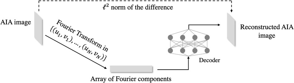
FIGURE 10. Neural network architecture that can be used for learning the best (u, v) coverage for representing an AIA image.
Such a process will result in the most useful datacubes for flare prediction. Moreover, it has value in informing instrument design: up to this juncture, the set of (u, v) values corresponding to the native data obtained from bi-grid occulting instruments such as RHESSI and STIX has been determined on the basis of a somewhat arbitrary selection of desired spatial (actually, angular) resolutions, coupled with other factors such as technological limitations. Clearly it would be advantageous to select the sampled (u, v) points based on the features of the Fourier spectrum that are likely to be present in actual sources. Repeating a similar training process using images with configurations typical of solar hard X-ray sources could thus reliably inform the design of future instrumentation.
In future works we will investigate how to predict the occurrence of a flare by implementing and training NNs with architectures similar to the one used by Guastavino et al. (2022) (see Figure 11). Specifically, the architecture consists of 3-D Convolutional Neural Networks (CNNs) which are applied to each one of the time steps t1, … , tM of the AIA datacube. Then, the processed information passes through fully-connected layers and through a Long-Short Term Memory (LSTM) network that takes into account the temporal evolution of the AIA data. Finally, the application of a sigmoid function returns an output between 0 and 1, representing the probability of a future flaring occurrence. However, in contrast to Guastavino et al. (2022), which was designed for use with monochromatic HMI images, and hence used 2-D CNNs, we shall make use of 3-D CNNs in order to effectively look for patterns across the different channels in the AIA data (or, equivalently, across the temperature domain).
The generation of reliable flare predictions through application of such an NN must await a significant amount of future work, including:
1. since the AIA images in different wavelength channels are produced sequentially, these images must be “synchronized” by interpolating (e.g., using Lagrange polynomials) to produce a time sequence of AIA images in each channel that all correspond to the same time;
2. apply the Cheung et al. (2015) DEM inversion algorithm to these synchronized images in order to obtain DEM(x, y; T; t) data hypercubes;
3. use Equation 2 to convert these into
4. train a NN (see Figure 11) on these data hypercubes to recognize features that lead to a correct prediction of the label associated with the data hypercube (e.g., a [0,1] binary “flare/non-flare” prediction, or the prediction of a continuous value such as GOES intensity, duration, integral of intensity over time, etc.).
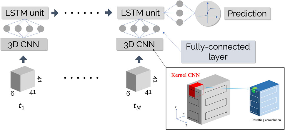
FIGURE 11. Schematic of a CNN that applies 3-D (u, v; T) filter layers to an
However, the main message of the present work is to stress the overall value of using spatial Fourier components (visibilities) to accurately encode source spatial information in a relatively small number of data points, and so reduce the computational burden relative to what would be needed to train NNs on the much larger datasets associated with direct spatial images.
6 Conclusion
We have seen that using a sparsely populated set of spatial Fourier components (visibilities) to represent AIA images of solar ARs not only allows a very significant compression (by a factor of ∼ 50) without significant loss of information on source features, but also allows identification of features that might be challenging to detect directly from spatial maps. Such highly compressed data sets can therefore be used to train NNs to recognize features that presage a solar flare. Further, compression of the data into spatial Fourier components admits the implementation of reasonably-sized three-dimensional NNs that also sample the data across temperature space, and so can be trained to recognize features corresponding to thermodynamic processes such as heating and cooling, in addition to the spatial signatures revealed by monochromatic images such as magnetograms.
Data availability statement
The SDO/AIA datasets analyzed, and the IDL codes implemented for this study, can be found at https://github.com/paolomassa/Fourier_transform_AIA.git.
Author contributions
The motivation and overall direction for this study was provided by AE. PM carried out the analysis of the data sets and the image reconstructions using visibility data and the MEM_GE code. Both authors played an equal role in writing the manuscript.
Funding
This work was supported by NASA Kentucky under NASA award number 80NSSC21M0362.
Acknowledgments
We appreciate the invitation to present this work in this Special Volume, and we hope that it motivates others to pursue investigations along similar lines. We thank the reviewers for careful reading of the originally submitted version of the manuscript and for several very helpful suggestions that led to its improvement. We are particularly grateful to one of the reviewers for the suggestion of using diverging color maps in Figure 9, which distinctly improved the visualization of the information in the key visibility difference maps. We also thank Mark Cheung and Marc DeRosa for some very valuable discussions on the use of AIA data for flare prediction purposes and on the DEM inversion procedure discussed in Section 2.3, Sabrina Guastavino, Gongbo Liang, and Hameedullah Farooki for valuable discussions regarding the implementation of the NNs described in the paper, and Ivan Novikov for a critical reading of the manuscript.
Conflict of interest
The authors declare that the research was conducted in the absence of any commercial or financial relationships that could be construed as a potential conflict of interest.
Publisher’s note
All claims expressed in this article are solely those of the authors and do not necessarily represent those of their affiliated organizations, or those of the publisher, the editors and the reviewers. Any product that may be evaluated in this article, or claim that may be made by its manufacturer, is not guaranteed or endorsed by the publisher.
Footnotes
1Note that the definition of Fourier transform we adopt is typical of astronomical applications and differs from the usual one used in harmonic analysis by the use of a plus sign inside the complex exponential. Since the information presented here (e.g., Figures 5, 9) regards visibility amplitudes, this distinction has no significant impact on the results. Further, although the choice of origin (xo, yo) does not affect the amplitude information presented in those Figures, the images reconstructed from the visibility data (see Figure 6) do use the phase information, and so the choice of origin is important for the fidelity of these reconstructed images.
2“Ringing” effects are a manifestation of the Gibbs phenomenon in the context of image reconstruction. They appear as periodic repetition of artifacts representing the true source structure and are fundamentally due to the loss of information associated with the truncation of high-spatial-frequency embedded in the signal (see page 123 of Bertero and Boccacci, 1998).
3It should also be possible to substantially eliminate these artifacts without significantly increasing the number of sampled spatial frequency points, if the selected spatial frequencies are chosen with sufficient care—see Section 5.
4For the computation of SSIM, we set the constant values C1, C2 and C3 equal to zero (see Eqs 6, 9 and 10 in Wang et al., 2004), since there are no instabilities due to values close to zero in the denominators.
References
Baker, D. N. (1998). What is space weather? Adv. Space Res. 22, 7–16. doi:10.1016/S0273-1177(97)01095-8
Balasubramaniam, K. S., and West, E. A. (1991). Vector magnetic fields in sunspots. I. Stokes profile Analysis using the marshall space flight center magnetograph. Astrophys. J. 382, 699. doi:10.1086/170757
Bertero, M., and Boccacci, P. (1998). Introduction to inverse problems in imaging. Boca Raton, FL: CRC Press.
Bobra, M. G., and Couvidat, S. (2015). Solar flare prediction using SDO/HMI vector magnetic field data with a machine-learning algorithm. Astrophys. J. 798, 135. doi:10.1088/0004-637X/798/2/135
Bobra, M. G., Sun, X., Hoeksema, J. T., Turmon, M., Liu, Y., Hayashi, K., et al. (2014). The helioseismic and magnetic imager (HMI) vector magnetic field pipeline: SHARPs - space-weather HMI active region patches. Sol. Phys. 289, 3549–3578. doi:10.1007/s11207-014-0529-3
Campi, C., Benvenuto, F., Massone, A. M., Bloomfield, D. S., Georgoulis, M. K., and Piana, M. (2019). Feature ranking of active region source properties in solar flare forecasting and the uncompromised stochasticity of flare occurrence. Astrophys. J. 883, 150. doi:10.3847/1538-4357/ab3c26
Camporeale, E., Wing, S., and Johnson, J. (2018). Machine learning techniques for space weather. Philadelphia, PA: Elsevier.
Carrington, R. C. (1859). Description of a singular appearance seen in the Sun on September 1, 1859. Mon. Not. R. Astron. Soc. 20, 13–15. doi:10.1093/mnras/20.1.13
Chen, J., Li, W., Li, S., Chen, H., Zhao, X., Peng, J., et al. (2022). Two-stage solar flare forecasting based on convolutional neural networks. Space Sci. Technol. 2022, 1–10. doi:10.34133/2022/9761567
Cheung, M. C. M., Boerner, P., Schrijver, C. J., Testa, P., Chen, F., Peter, H., et al. (2015). Thermal diagnostics with the atmospheric imaging assembly on board the solar dynamics observatory: A validated method for differential emission measure inversions. Astrophys. J. 807, 143. doi:10.1088/0004-637X/807/2/143
Drake, J. F., Swisdak, M., and Fermo, R. (2013). The power-law spectra of energetic particles during multi-island magnetic reconnection. Astrophys. J. 763, L5. doi:10.1088/2041-8205/763/1/L5
Ehrengruber, J., and Melchior, M. (2020). “Exploring predictive capabilities of GOES and SDO/EVE data for flare forecasting,” in 2020 IEEE International Conference on Big Data (Big Data), 4192–4199. doi:10.1109/BigData50022.2020.9378339
Falconer, D. A. (1997). A correlation between length of strong-shear neutral lines and total X-ray brightness in active regions. Sol. Phys. 176, 123–126. doi:10.1023/A:1004989113714
Falconer, D. A., Moore, R. L., and Gary, G. A. (2002). Correlation of the coronal mass ejection productivity of solar active regions with measures of their global nonpotentiality from vector magnetograms: Baseline results. Astrophys. J. 569, 1016–1025. doi:10.1086/339161
Falconer, D. A., Moore, R. L., and Gary, G. A. (2007). Forecasting coronal mass ejections from line-of-sight magnetograms. J. Atmos. Solar-Terrestrial Phys. 69, 86–90. doi:10.1016/j.jastp.2006.06.015
Falconer, D. A., Moore, R. L., and Gary, G. A. (2006). Magnetic causes of solar coronal mass ejections: Dominance of the free magnetic energy over the magnetic twist alone. Astrophys. J. 644, 1258–1272. doi:10.1086/503699
Falconer, D. A., Moore, R. L., and Gary, G. A. (2008). Magnetogram measures of total nonpotentiality for prediction of solar coronal mass ejections from active regions of any degree of magnetic complexity. Astrophys. J. 689, 1433–1442. doi:10.1086/591045
Florios, K., Kontogiannis, I., Park, S.-H., Guerra, J. A., Benvenuto, F., Bloomfield, D. S., et al. (2018). Forecasting solar flares using magnetogram-based predictors and machine learning. Sol. Phys. 293, 28. doi:10.1007/s11207-018-1250-4
Forbes, T. G., Linker, J. A., Chen, J., Cid, C., Kóta, J., Lee, M. A., et al. (2006). CME theory and models. Space Sci. Rev. 123, 251–302. doi:10.1007/s11214-006-9019-8
Galvez, R., Fouhey, D. F., Jin, M., Szenicer, A., Muñoz-Jaramillo, A., Cheung, M. C. M., et al. (2019). A machine-learning data set prepared from the NASA solar dynamics observatory mission. Astrophys. J. Suppl. Ser. 242, 7. doi:10.3847/1538-4365/ab1005
Georgoulis, M. K., Bloomfield, D. S., Piana, M., Massone, A. M., Soldati, M., Gallagher, P. T., et al. (2021). The flare likelihood and region eruption forecasting (FLARECAST) project: Flare forecasting in the big data & machine learning era. J. Space Weather Space Clim. 11, 39. doi:10.1051/swsc/2021023
Guastavino, S., Marchetti, F., Benvenuto, F., Campi, C., and Piana, M. (2022). Implementation paradigm for supervised flare forecasting studies: A deep learning application with video data. Astron. Astrophys. 662, A105. doi:10.1051/0004-6361/202243617
Hagyard, M. J., Moore, R. L., and Emslie, A. G. (1984a). The role of magnetic field shear in solar flares. Adv. Space Res. 4, 71–80. doi:10.1016/0273-1177(84)90162-5
Hagyard, M. J., Smith, J., Teuber, D., and West, E. A. (1984b). A quantitative study relating observed shear in photospheric magnetic fields to repeated flaring. Sol. Phys. 91, 115–126. doi:10.1007/BF00213618
Hertel, L., Phan, H., and Mertins, A. (2016). “Comparing time and frequency domain for audio event recognition using deep learning,” in 2016 international joint conference on neural networks (IJCNN) (IEEE), 3407–3411.
Hodgson, R. (1859). On a curious appearance seen in the Sun. Mon. Not. R. Astron. Soc. 20, 15–16. doi:10.1093/mnras/20.1.15a
Huang, X., Wang, H., Xu, L., Liu, J., Li, R., and Dai, X. (2018). Deep learning based solar flare forecasting model. I. Results for line-of-sight magnetograms. Astrophys. J. 856, 7. doi:10.3847/1538-4357/aaae00
Hurford, G. J., Schmahl, E. J., Schwartz, R. A., Conway, A. J., Aschwanden, M. J., Csillaghy, A., et al. (2002). The RHESSI imaging concept. Sol. Phys. 210, 61–86. doi:10.1023/A:1022436213688
Inceoglu, F., Shprits, Y. Y., Heinemann, S. G., and Bianco, S. (2022). Identification of coronal holes on AIA/SDO images using unsupervised machine learning. Astrophys. J. 930, 118. doi:10.3847/1538-4357/ac5f43
Jonas, E., Bobra, M., Shankar, V., Todd Hoeksema, J., and Recht, B. (2018). Flare prediction using photospheric and coronal image data. Sol. Phys. 293, 48. doi:10.1007/s11207-018-1258-9
Krucker, S., Hurford, G. J., Grimm, O., Kögl, S., Gröbelbauer, H. P., Etesi, L., et al. (2020). The spectrometer/telescope for imaging X-rays (STIX). Astron. Astrophys. 642, A15. doi:10.1051/0004-6361/201937362
Lemen, J. R., Title, A. M., Akin, D. J., Boerner, P. F., Chou, C., Drake, J. F., et al. (2012). The atmospheric imaging assembly (AIA) on the solar dynamics observatory (SDO). Sol. Phys. 275, 17–40. doi:10.1007/s11207-011-9776-8
Li, X., Zheng, Y., Wang, X., and Wang, L. (2020). Predicting solar flares using a novel deep convolutional neural network. Astrophys. J. 891, 10. doi:10.3847/1538-4357/ab6d04
Lin, R. P., Dennis, B. R., Hurford, G. J., Smith, D. M., Zehnder, A., Harvey, P. R., et al. (2002). The reuven ramaty high-energy solar spectroscopic imager (RHESSI). Sol. Phys. 210, 3–32. doi:10.1023/A:1022428818870
Liu, C., Deng, N., Wang, J. T. L., and Wang, H. (2017). Predicting solar flares using SDO/HMI vector magnetic data products and the random forest algorithm. Astrophys. J. 843, 104. doi:10.3847/1538-4357/aa789b
Mariska, J. T., Emslie, A. G., and Li, P. (1989). Numerical simulations of impulsively heated solar flares. Astrophys. J. 341, 1067. doi:10.1086/167564
Massa, P., Battaglia, A. F., Volpara, A., Collier, H., Hurford, G. J., Kuhar, M., et al. (2022). First hard X-ray imaging results by solar orbiter STIX. Sol. Phys. 297, 93. doi:10.1007/s11207-022-02029-x
Massa, P., Schwartz, R., Tolbert, A. K., Massone, A. M., Dennis, B. R., Piana, M., et al. (2020). MEM_GE: A new maximum entropy method for image reconstruction from solar X-ray visibilities. Astrophys. J. 894, 46. doi:10.3847/1538-4357/ab8637
Moore, R. L., Sterling, A. C., Hudson, H. S., and Lemen, J. R. (2001). Onset of the magnetic explosion in solar flares and coronal mass ejections. Astrophys. J. 552, 833–848. doi:10.1086/320559
Mrozek, T., Tomczak, M., and Gburek, S. (2007). Solar impulsive EUV and UV brightenings in flare footpoints and their connection with X-ray emission. Astron. Astrophys. 472, 945–955. doi:10.1051/0004-6361:20077652
Nagem, T., Qahwaji, R., Ipson, S., and Wang, Z. (2018). Deep learning technology for predicting solar flares from geostationary operational environmental satellite data. Int. J. Adv. Comput. Sci. Appl. 9, 492–498. doi:10.14569/ijacsa.2018.090168
Nishizuka, N., Sugiura, K., Kubo, Y., Den, M., and Ishii, M. (2018). Deep flare net (DeFN) model for solar flare prediction. Astrophys. J. 858, 113. doi:10.3847/1538-4357/aab9a7
Petrosian, V. (2016). Particle acceleration in solar flares and associated CME shocks. Astrophys. J. 830, 28. doi:10.3847/0004-637X/830/1/28
Phillips, K. J. H., Feldman, U., and Landi, E. (2008). Ultraviolet and X-ray spectroscopy of the solar atmosphere. Cambridge University Press.
Piana, M., Emslie, A. G., Massone, A. M., and Dennis, B. R. (2022). Hard X-ray imaging of solar flares. Berlin: Springer-Verlag.
Savage, S., Winebarger, A., Glesener, L., Golub, L., Chamberlin, P., Hi-C Flare Team, , et al. (2021). The first solar flare sounding rocket campaign and its potential impacts for high energy solar instrumentation. Am. Astronomical Soc. Meet. Abstr. 53, 313.15.
Scherrer, P. H., Bogart, R. S., Bush, R. I., Hoeksema, J. T., Kosovichev, A. G., Schou, J., et al. (1995). The solar oscillations investigation - Michelson Doppler imager. Sol. Phys. 162, 129–188. doi:10.1007/BF00733429
Scherrer, P. H., Schou, J., Bush, R. I., Kosovichev, A. G., Bogart, R. S., Hoeksema, J. T., et al. (2012). The helioseismic and magnetic imager (HMI) investigation for the solar dynamics observatory (SDO). Sol. Phys. 275, 207–227. doi:10.1007/s11207-011-9834-2
Tandberg-Hanssen, E., and Emslie, A. G. (1988). The physics of solar flares. Cambridge University Press.
Tousey, R., Watanabe, K., and Purcell, J. D. (1951). Measurements of solar extreme ultraviolet and X-rays from rockets by means of a CoSO4:Mn phosphor. Phys. Rev. 83, 792–797. doi:10.1103/PhysRev.83.792
Wang, Z., Bovik, A., Sheikh, H., and Simoncelli, E. (2004). Image quality assessment: From error visibility to structural similarity. IEEE Trans. Image Process. 13, 600–612. doi:10.1109/TIP.2003.819861
Xu, K., Qin, M., Sun, F., Wang, Y., Chen, Y.-K., and Ren, F. (2020). “Learning in the frequency domain,” in Proceedings of the IEEE/CVF conference on computer vision and pattern recognition, 1740–1749.
Yi, K., Moon, Y.-J., Lim, D., Park, E., and Lee, H. (2021). Visual explanation of a deep learning solar flare forecast model and its relationship to physical parameters. Astrophys. J. 910, 8. doi:10.3847/1538-4357/abdebe
Zeiler, M. D., Krishnan, D., Taylor, G. W., and Fergus, R. (2010). “Deconvolutional networks,” in 2010 IEEE computer society conference on computer vision and pattern recognition (IEEE), 2528–2535.)
Zhang, Q., Barri, K., Babanajad, S. K., and Alavi, A. H. (2020). Real-time detection of cracks on concrete bridge decks using deep learning in the frequency domain. Engineering 7, 1786–1796. doi:10.1016/j.eng.2020.07.026
Keywords: flare forecasting, SDO/AIA data, data compression, Fourier transforms, neural networks, space weather
Citation: Massa P and Emslie AG (2022) Efficient identification of pre-flare features in SDO/AIA images through use of spatial Fourier transforms. Front. Astron. Space Sci. 9:1040099. doi: 10.3389/fspas.2022.1040099
Received: 08 September 2022; Accepted: 15 November 2022;
Published: 07 December 2022.
Edited by:
Yang Chen, University of Michigan, United StatesReviewed by:
Zeyu Sun, University of Michigan, United StatesDebi Prasad Choudhary, California State University, United States
Copyright © 2022 Massa and Emslie. This is an open-access article distributed under the terms of the Creative Commons Attribution License (CC BY). The use, distribution or reproduction in other forums is permitted, provided the original author(s) and the copyright owner(s) are credited and that the original publication in this journal is cited, in accordance with accepted academic practice. No use, distribution or reproduction is permitted which does not comply with these terms.
*Correspondence: Paolo Massa, cGFvbG8ubWFzc2FAd2t1LmVkdQ==