 B. L. Burkholder
 R. Cuellar3
 K. Nykyri
 X. Ma
X. Ma
95% of researchers rate our articles as excellent or good
Learn more about the work of our research integrity team to safeguard the quality of each article we publish.
Find out more
ORIGINAL RESEARCH article
Front. Astron. Space Sci. , 24 November 2022
Sec. Space Physics
Volume 9 - 2022 | https://doi.org/10.3389/fspas.2022.1040082
This article is part of the Research Topic Advances on Upper-Atmosphere Characterization for Geodetic Space Weather Research and Applications View all 6 articles
To investigate the meso-scale structure (100 s of km) of the ionosphere at mid-latitudes, the spectral properties in calculated total electron content (TEC) at a cluster of GPS receivers in and around Florida are analyzed. The ionosphere does not respond exactly the same to periodic solar driving at different locations around the planet, due to the complex electrodynamic interactions of the coupled magnetosphere-ionosphere system. Therefore, at each GPS receiver in the cluster we compare spatio-temporal variations of the spectral amplitudes for diurnal, solar rotation, and seasonal oscillations. The amplitudes for these dominant oscillations are organized with respect to magnetic latitude of the receiver. A low-latitude and high-latitude station are also included to put the mid-latitude ionospheric response into a global context. The amplitudes of diurnal, seasonal, and solar rotation signals are well ordered by magnetic latitude, superposed with meso-scale deviations between stations separated by
Meso-scale (100 s of km) structures form in the ionosphere due to different plasma instabilities (Kelley, 1989a; Kelley, 1989b), some examples of their manifestation including equatorial plasma bubbles (Woodman and La Hoz, 1976), storm enhanced density plumes (Foster et al., 2021), and (medium-scale) traveling ionospheric disturbances (Hines, 1959, 1960; Hunsucker, 1982). In addition, lightning- and thunderstorm-induced generation of acoustic-gravity waves (Lay et al., 2015) can directly impact the ionosphere at mid-latitudes (Lay et al., 2018) and can be detected from analysis of very low frequency (VLF) pulses (Cheng and Cummer, 2005). The combination of all these processes impact the mid-latitude ionosphere and create irregularities that can disrupt radio-communication (Aa et al., 2019).
Dense arrays of ground-based Global Positioning System (GPS) receivers, such as the National Oceanic and Atmospheric Administration (NOAA) Continuously Operating Reference Stations (CORS) Network (NCN), can be used to probe meso-scale ionosphere structures. In principle, it is possible to resolve strong gradients and ionospheric irregularities at a regional scale using distributed sensors (Lay et al., 2018). A natural use of such a data set would be to train an artificial intelligence (AI) to predict the ionospheric total electron content at a regional scale based on solar wind conditions. But, it is the case that the mid-latitude total electron content is dominated by the diurnal signal, with meso-scale structures superposed as fluctuations. Therefore, it is the goal of this study to characterize the ionospheric response to persistent external driving on a regional scale, i.e. what are the amplitudes of strong sinusoidal variations of total electron content (TEC) for the different observatories in a closely separated network of sensors and how do they change in time?
The harmonic response of the ionosphere has received attention for decades through space and ground-based measurements. Davies et al. (1980) compared diurnal variations of TEC during magnetically quiet and disturbed conditions from a total of 5 radio beacons in the United States and Europe. Perevalova et al. (2010) used a widely distributed network of GPS receivers to construct Global Ionospheric Maps (GIMs) with a resolution of 5° longitude and 2.5° latitude. Based on the GIMs, the authors seasonally characterized the heliomagnetically quiet diurnal TEC response for low (0–20°), mid (40–55°), and high (60–87.5°) latitudes, providing a global scale picture of the daily response of the ionosphere. Huang and Roussel-Dupré (2005) quantified the diurnal, seasonal, and solar cycle variations of TEC using Fast On-Orbit Recording of Transient Events (FORTE)-received Los Alamos Portable Pulser (LAPP) signals in Los Alamos, New Mexico. Olwendo et al. (2016) studied the diurnal and annual variations of TEC from 12 receivers in East Africa separated by 25° geographic latitude containing the magnetic equator. They noted the difficulty of accurately computing vertical TEC (vTEC) from slant TEC (sTEC) due to large spatiotemporal gradients of the equatorial ionization anomaly. Guo et al. (2015) constructed TEC time series on a global 5° × 2.5 ° grid using more than 350 GPS stations. Morlet wavelet analysis was used to determine periods of TEC variations and the 1-day, 26.5-day, semi-annual and annual cycles were found to be the dominant signals. Recently, Yasyukevich et al. (2017) employed harmonic spectral analysis to study annual, seasonal, and diurnal variations of the ionosphere. They looked at a full solar cycle of data from 2 GPS receivers in Russia and found oscillations with periods of 1, 1/2 … up to 1/5 of a day, and 27-day are clearly distinguished in the TEC spectra at high and middle latitudes. During solar maximum, the amplitude of harmonics was twice as high, and the number of clearly manifested harmonics was more than during the solar minimum. They also found using F10.7 solar radio flux that the amplitude of all the ionospheric harmonics follows the solar activity level changes.
Numerous other studies have indicated the presence of periodic signatures in the ionosphere at various locations on Earth (Xingliang et al., 2005; Cai, 2007; Afraimovich et al., 2008; Amiri-Simkooei and Asgari, 2011; Chauhan et al., 2011; Olwendo et al., 2012; Liu et al., 2014; Tariku, 2015; Elemo et al., 2018; Ogwala et al., 2019; Akinyemi et al., 2021). Note that the majority of characterization studies have been performed in low-latitude or high-latitude regions where geomagnetic activity dominates the physical processes. At mid-latitudes, tropospheric and geomagnetic phenomena compete in disturbing the ionosphere, and it is not well understood how these multiple sources affect the ionospheric drivers. Even for the relatively lower density night-time mid-latitude ionosphere the Perkins instability produces periodic variations of TEC (Perkins, 1973). The result of these many processes is that a solar cycle spectrum of TEC is composed of signals spanning small-to meso-to larger spatio-temporal scales.
Measurements from the NOAA CORS network can be obtained from the National Geodetic Survey: https://geodesy.noaa.gov/CORS/. The data rate varies between stations but we use stations taking more than 1 sample per minute and down-sample to 1 sample per minute. The data are daily GNSS Observation files which are provided in the receiver-independent exchange (RINEX) format and must be converted to vTEC. The GPS-TEC analysis software, developed by Gopi Seemala (Ma and Maruyama, 2003; Seemala and Valladares, 2011), uses phase and code values for both L1 and L2 GPS frequencies to eliminate the effect of clock errors and tropospheric water vapor, and thus calculate relative values of sTEC (Sardón et al., 1994; Sardón and Zarraoa, 1997; Arikan et al., 2008). Then, the absolute values of sTEC are obtained by accounting for the differential code biases at the satellites (Valladares et al., 2009). The final vTEC data is then calculated by including the geometric factor. The equations used by the GPS-TEC software can be found in Ma and Maruyama. (2003). It is known that the true value of TEC is difficult to calculate due to the receiver biases, but this is largely affecting the DC component of the spectrum so it is not relevant to our study.
The data for this study includes 15 mid-latitude stations within 10 degrees of geographic latitude and longitude (corresponding to an area of ∼700 mi2) of one another (see table of geomagnetic latitude and longitude in Figure 1) covering solar cycle 24 from 2009 to 2019. The station in Jacksonville, Florida (ZJX1), a central location in the cluster, is at magnetic latitude
with
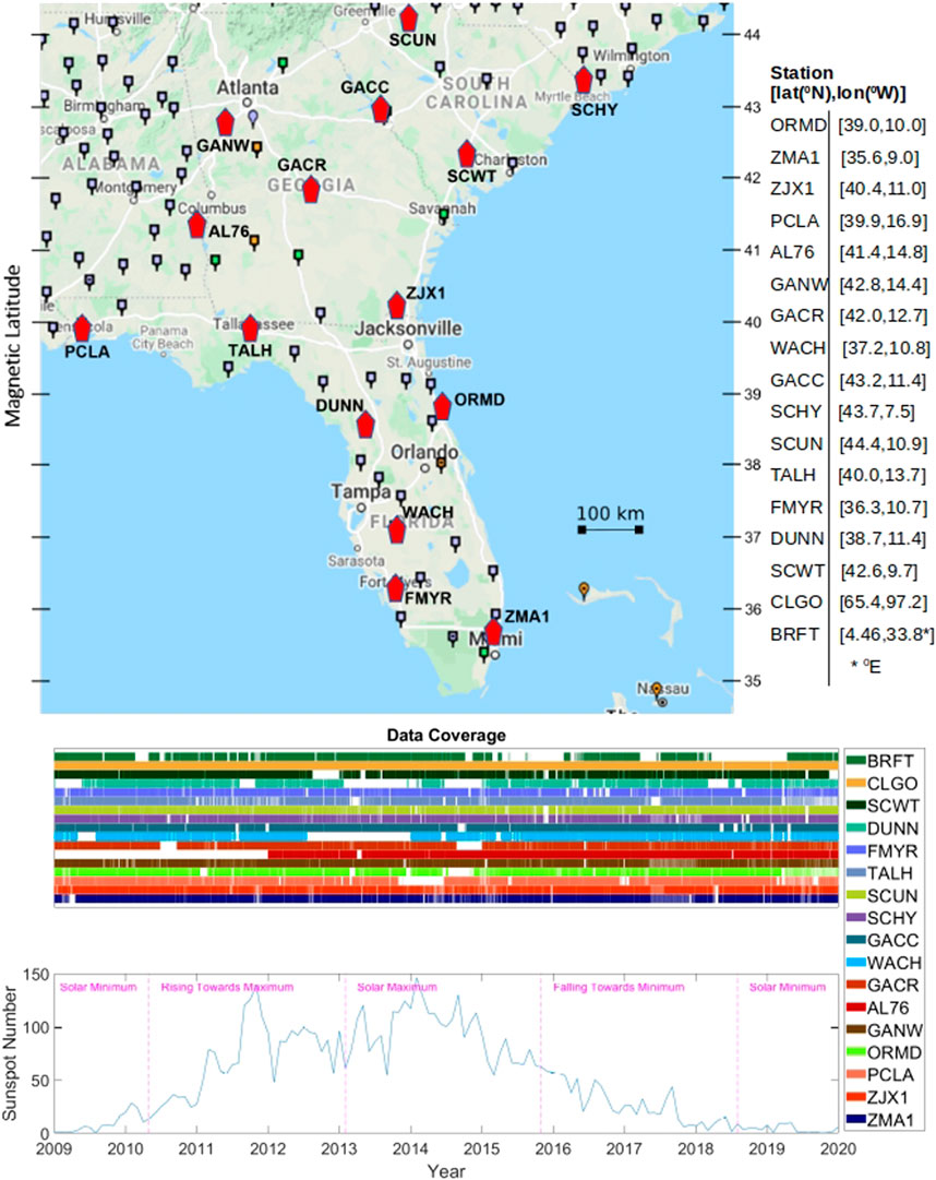
FIGURE 1. Map of CORS GPS receivers with table giving magnetic latitude and longitude of each station (top), data coverage of stations in this study (middle), and sunspot number (obtained from the NOAA Space Weather Prediction Center) with labeled phases of solar cycle 24 (bottom). The stations BRFT (Brazil) and CLGO (Alaska) are not shown on the map. Large red pentagons on the station map show the GPS receivers used in this study, and many other CORS stations are given by small squares or circles.
In addition to calculating the spectrum for an entire solar cycle of data, we also sequester portions of the time series corresponding to the different phases of solar cycle 24. We have defined these intervals as shown in the bottom panel of Figure 1, which gives the sunspot number time series for 1 January 2009 to 1 January 2020. The phases are defined as Solar Minimum: 1 January 2009–15 May 2010 and 16 August 2018–1 January 2020, Rising toward Maximum: 16 May 2010–15 February 2013, Solar Maximum: 16 February 2013–15 November 2015, Falling toward Minimum: 16 November 2015–15 August 2018.
The Miami (ZMA1) TEC time series for 1 January 2009 to 1 January 2020 is shown in the top panel of Figure 2. Note that the sunspot number (bottom of Figure 1) peaks strongly during solar maximum from 2014 to 2015 but also has a peak of similar magnitude during the second half of 2011. On the longest visible time-scale, the TEC time series from Miami reflects the shape of the sunspot number curve. Also easy to pick out are the annual and semi-annual cycles of TEC. The diurnal variation dominates the signal being too high frequency to easily identify in the 11-year time series. However, the second panel of Figure 2 shows the Lomb-Scargle periodogram for the TEC time series, which indicates the signal with a frequency of 365/year has the largest power at about 20 TECU. The magenta (cyan) vertical dashed lines indicate the location of a fundamental frequency at 1/year (365/year) and the corresponding harmonics for n = 2,3, … The fundamental and first harmonic of the seasonal cycle have similar power. In the case of the diurnal cycle, many harmonics are well resolved. The fundamental dominates the harmonics in power but it is noteworthy that the first harmonic has similar power to the seasonal signal. The power in the signal at the solar rotation ∼ 27 day period (∼14/year, see red arrow) is broadband and lacking in discernible harmonics, because it results from multiple sources on the Sun which do not always last a full solar rotation.
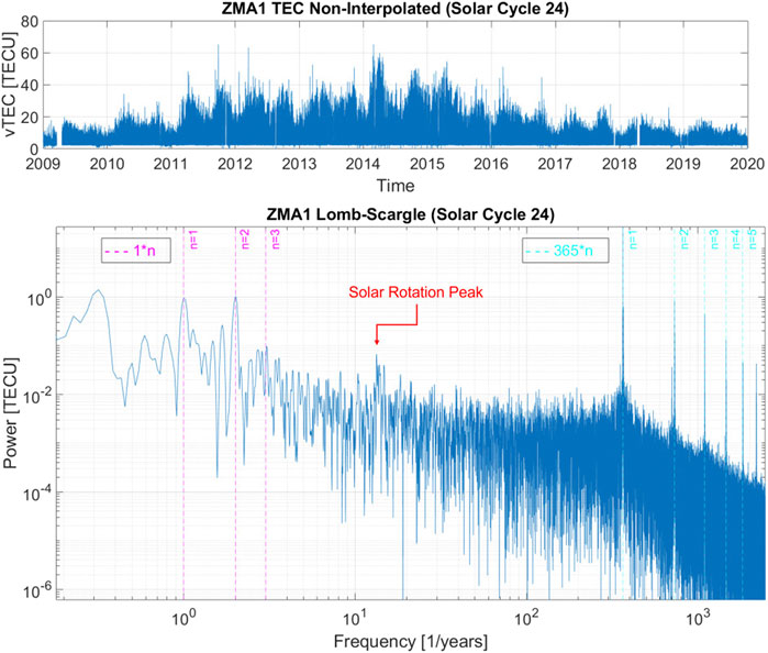
FIGURE 2. TEC time series (top) and Lomb-Scargle periodogram (bottom) for station ZMA1 during solar cycle 24 (1 January 2009 to 1 January 2020). Annual and semi-annual signatures can be easily identified in the time series, along with higher amplitude diurnal variations. In the spectrum a vertical pink (cyan) dashed line is overlaid at the fundamental frequency of 1/year (365/year) along with some harmonics n = ,2,3, … The solar rotation peak also appears as a broadband source.
Figure 3 shows Lomb-Scargle periodograms for the TEC time series from Figure 2 split into the different phases of the solar cycle. The diurnal cycle (365/year), first harmonic, and many more harmonics (not shown), are well resolved during all phases of the solar cycle. The solar rotation is well resolved during all phases except for solar minimum. At solar minimum, the annual signal dominates the semi-annual signal. During the rising phase, the semi-annual signal is slightly more powerful than the annual signal. At solar maximum, the annual signal is slightly more powerful than the semi-annual signal. During the falling phase, the annual signal is significantly more powerful than the semi-annual signal but not so much as during solar minimum. Splitting the data into phases of the solar cycle shows also that the frequency for “annual”, “semi-annual”, and “solar rotation” is not fixed in time. Only from an entire solar cycle of data are the annual and semi-annual signals present as well-resolved peaks very close to 1/year and 2/year. Later, we will discuss the solar rotation peak for the different solar cycle phases.
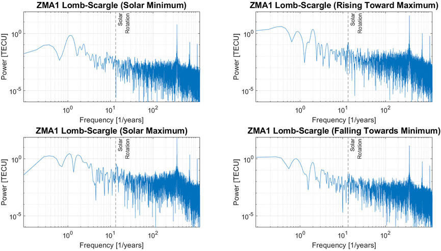
FIGURE 3. Lomb-Scargle periodograms for the TEC time series from ZMA1 during solar minimum (top left), rising (top right), solar maximum (bottom left), and falling (bottom right) phases of solar cycle 24.
We construct periodograms for each station similar to Figures 2, 3 and extract the amplitudes for the diurnal, annual, and seasonal oscillations, as well as the relevant harmonics. The power in the fundamental diurnal frequency for each station is plotted in Figures 4, 5 as a function of magnetic latitude of the station. Figure 4 shows solar minimum (top) and rising phase (bottom) and Figure 5 shows solar maximum (top) and falling phase (bottom). The error bars are computed from a 90-day sliding window (with 30-day separations) periodogram for the corresponding phase. The smallest fundamental diurnal amplitude from all sub-intervals is the value of the downwards error bar and like-wise for the upwards error bar. The error bars thus represent the variability of the signal over the corresponding solar cycle phase. The amplitude at all stations corresponds to solar activity level and magnetic latitude. If we assume the stations should fall on a straight line connecting CLGO and BRFT, deviations from such a line represent the meso-scale ionospheric structure of interest to this study. At solar minimum and falling phase, within the mid-latitude cluster of stations the power deviates from a straight line by 1-2 TECU, while the deviation is 10–20 TECU for rising phase and solar max. It may be alarming to the reader that the error bars are much larger than these variations, but since the error bars represent the time-variation of the amplitudes, it can be expected that all the stations are having their largest or smallest amplitudes at a similar time of the year. Note also that the variation between stations is similar at the top and bottom of the error bars, compared with the variations between stations for the blue points. This is an effect of meso-scale variations (from station-to-station) superposed onto the fundamental signal which does not have a constant frequency in time. A final consideration to take into account when comparing the error bars with the blue points is that the error bars are computed from the spectrum of a time series that is shorter than the spectrum which produced each blue point.
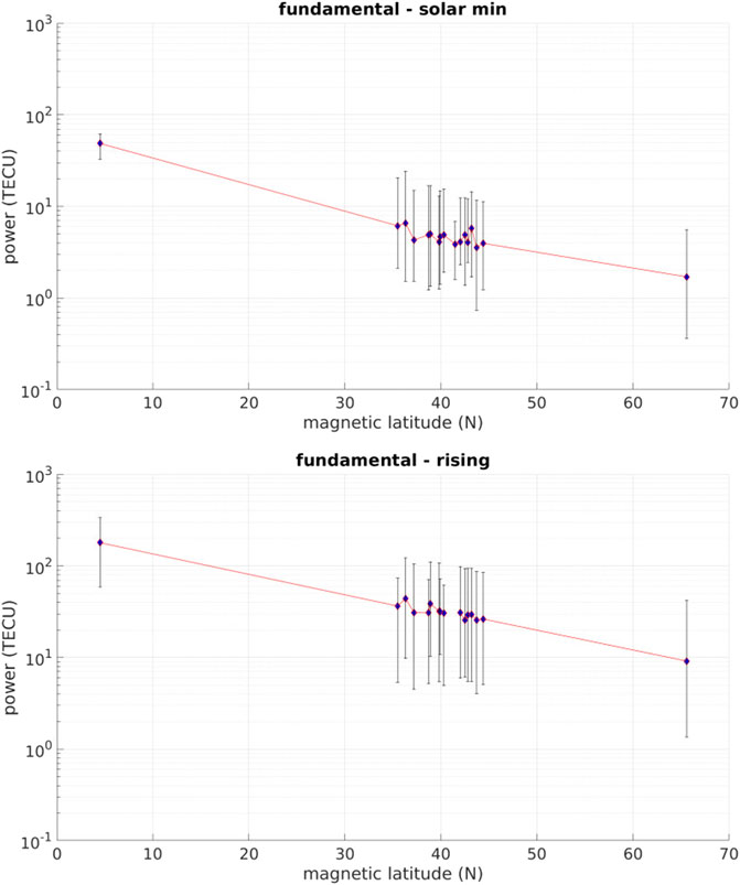
FIGURE 4. Each blue dot is the amplitude of the 365/year signal calculated from a Lomb-Scargle periodogram for the corresponding phase of solar cycle 24 (solar minimum on top and rising phase on bottom). The amplitudes are plotted with respect to the magnetic latitude of the station. Error bars are calculated as the smallest and largest amplitudes from a sliding window periodogram over 90 days sub-intervals of each solar phase. As a general trend the amplitudes align with magnetic latitude and solar activity. Meso-scale deviations from this trend indicate the presence of meso-scale ionosphere structure.
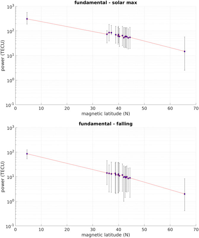
FIGURE 5. Each blue dot is the amplitude of the 365/year signal calculated from a Lomb-Scargle periodogram for the corresponding phase of solar cycle 24 (solar maximum on top and falling phase on bottom). The amplitudes are plotted with respect to the magnetic latitude of the station. Error bars are calculated as the smallest and largest amplitudes from a sliding window periodogram over 90 days sub-intervals of each solar phase. As a general trend the amplitudes align with magnetic latitude and solar activity. Meso-scale deviations from this trend indicate the presence of meso-scale ionosphere structure.
The diurnal signal mostly results from the day-night cycle of photoionization, and the reason to characterize this signal with high accuracy is because the amplitude is much greater than that of most isolated ionospheric structures. What we aim to predict is the location and extent of ionosphere structures associated with strong TEC gradients generated by geomagnetic disturbances originating from the Sun (i.e., storm enhanced density plume). Of course, these disturbances would not be resolved as peaks in the spectra (unless they are associated with a feature on the Sun that lasts longer than a solar rotation), but by knowing what the diurnal amplitude is at any station and any time, it becomes possible to subtract out this component of the signal and have remaining only the variations due to meso-scale ionospheric structures.
A sequence of harmonics in the spectra can be indicative of a signal that is more fundamentally a square wave than a sinusoid. This is an expected feature of the ionospheric TEC because the steady-state ionospheric density is determined by the balance of ionization and recombination. At night-time photoionization ceases but there is still a residual ionization from cosmic rays Webber. (1962), so the recombination rate will decrease throughout the night until it is in balance with the cosmic-ray ionization rate. To identify a square wave, the spectrum must have a series of harmonics with amplitudes that decrease with n. Figures 6, 7 illustrate the presence of meso-scale ionosphere structure based on the ratio of the amplitudes in the fundamental vs n = 1 harmonic, in the same way as Figures 4, 5. In Brazil, the amplitude ratio maximizes at solar maximum and minimizes at solar minimum, and, surprisingly (because it is a log scale plot), has a larger upward error bar for all phases except the falling phase. In Alaska, the amplitude ratio is mostly constant throughout the solar phases, having the smallest variation from minimum to maximum of all stations in this study. Quantitatively, the standard deviation of amplitude ratio across the 4 solar phases is 1.8 in Alaska, 7.8 in Brazil, and an average of 13.7 from all mid-latitude stations in this study. Similar to low-latitude, at middle-latitude the amplitude ratios correspond well with solar activity (higher ratio for more solar activity). Averaged across all mid-latitude stations the amplitude ratio is 19.1 at solar minimum, 43.9 in rising phase, 53.3 at solar maximum, and 31.9 in falling phase. Note also that from station-to-station at middle latitudes the ratio can vary by 10 or greater during all solar phases, similar to the variations demonstrated in Figures 4, 5. Additionally, during the solar minimum and falling phases, a few of the downward error bars approach 1. This is not the result of a square wave but suggests at these stations there is a driver at a frequency of twice per day rather than being a harmonic of the diurnal signal, potentially the semi-diurnal atmospheric tide (Oberheide et al., 2015).
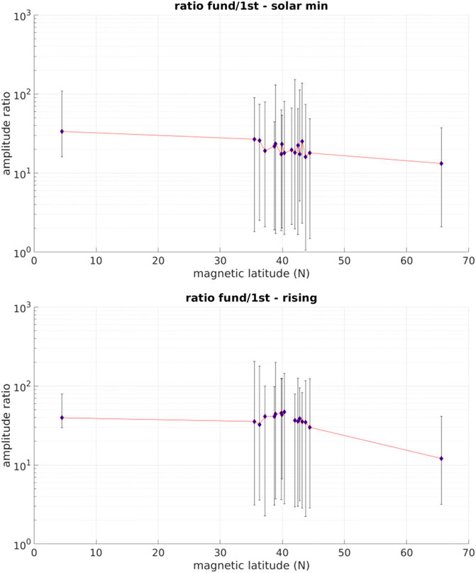
FIGURE 6. Ratio of fundamental diurnal vs. first harmonic amplitudes as a function of magnetic latitude during solar minimum (top) and rising phase (bottom). Error bars are the smallest and largest ratios from a sliding window periodogram over 90-day sub-intervals of each solar phase.
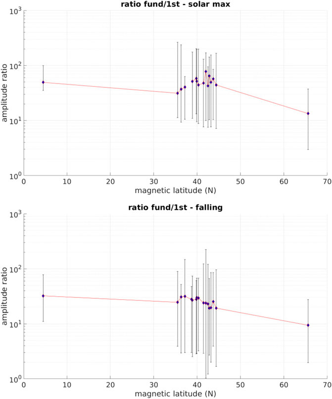
FIGURE 7. Ratio of fundamental diurnal vs. first harmonic amplitudes as a function of magnetic latitude during solar maximum (top) and falling phase (bottom). Error bars are calculated from 90-day sub-intervals. Errors bars approaching a ratio of 1 suggest the presence of a strong semi-diurnal driver.
For the 1/year signal derived from a periodogram of the entire solar cycle time series only a single harmonic is well resolved and the amplitude ratio between fundamental and first harmonic fluctuates about 1. This indicates a competition between drivers with frequencies of 1/year and 2/year, which are otherwise known as the annual and semi-annual cycles. Figure 8 quantifies the mid-latitude meso-scale structure of these different drivers. The top panel shows the amplitude of the annual signal as a function of magnetic latitude and the bottom panel shows the ratio of annual to semi-annual amplitudes. The error bars are constructed the same as Figure 4 but using a 3-year sliding window. From the top panel, there is a similar general dependence on magnetic latitude as for the fundamental diurnal signal and also a station-to-station deviation that is maximally 1-2 TECU from a power law fit. The bottom panel contains information about the competition of drivers with 1/year and 2/year frequencies. Within the cluster of mid-latitude stations the ratio of periodogram amplitudes from the entire cycle solar varies from less than 1 in some locations to greater than 1 in others. The error bars also indicate many of the stations go from a ratio that is less than 1 to greater than 1 or vice versa throughout the course of the solar cycle. In Brazil and Alaska, the error bars show the ratio is never greater than 1. The source of this meso-scale mid-latitude structure in the spectra is not the result of transient solar driving, as those effects occur on much shorter time scales, but must result from the interaction of the ionosphere with the neutral atmosphere and ground.
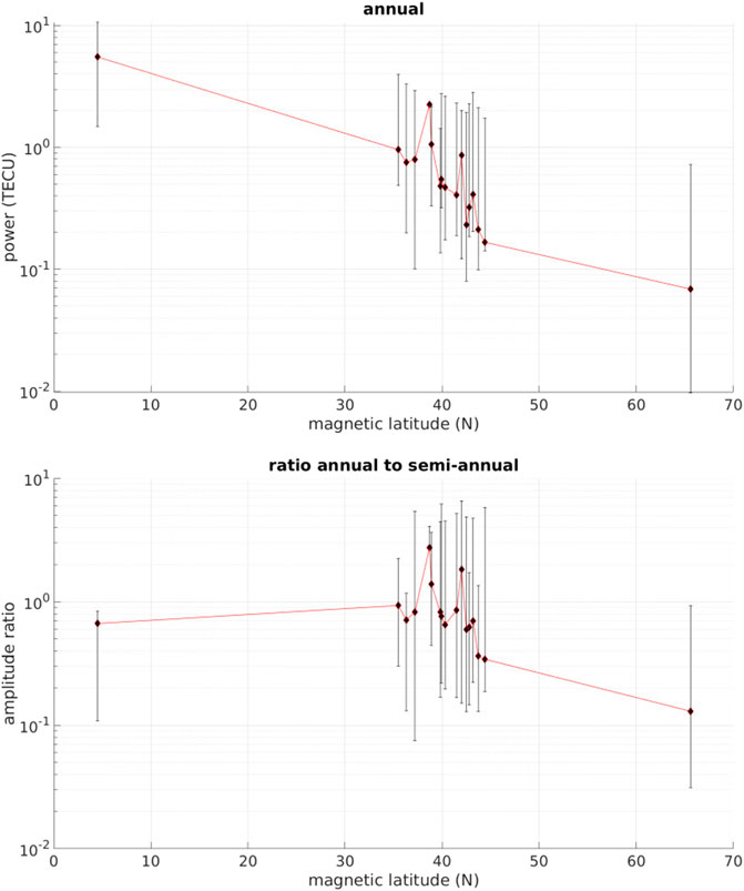
FIGURE 8. Periodogram annual amplitudes (top) and ratio of annual vs. semi-annual amplitudes (bottom) as a function of magnetic latitude. Error bars are the smallest and largest values from a sliding window periodogram over 3-year sub-intervals from the entire solar cycle. Note the spatio-temporal variations around 1 of the annual-to-semi-annual ratio for the mid-latitude stations.
Finally, Figures 9, 10 quantify the solar rotation amplitude during the different solar cycle phases. Because of the broadband nature of the solar rotation signal, it is intrinsically more difficult to quantify. We have taken the largest amplitude from a frequency window centered at 1/26.5 = 0.038 days−1 (labeled as solar rotation in Figure 3) with a width 0.01 days−1. For reference, the reader may note in the top left panel of Figure 3 there is a strong peak to the left of the solar rotation peak at a frequency of 1/45 days−1, which is outside of the tolerance window. The error bars in Figures 9, 10 use a 360-day sliding window. The fact that many of the lower error bars are very small is due to the different sources on the Sun, since each sinuosoidal driver will in this case exist for a much shorter time than an entire solar cycle phase. Similar to the diurnal frequency, the amplitudes are generally aligned with solar phase and magnetic latitude. At mid-latitude the typical station-to-station deviation is about 0.1–0.2 TECU during solar maximum and rising phases and just slightly smaller during solar minimum and falling phases. The driver for this signal, being mostly coronal hole high speed streams and co-rotating interaction regions, results in a broadband signal because these features are appearing and disappearing on the Sun. Since the solar rotation signal is lower frequency than the diurnal signal but higher frequency than the annual signal, the ionospheric response on these time scales is in between that produced by transient solar wind drivers and the interaction of ionosphere with neutral atmosphere and ground.
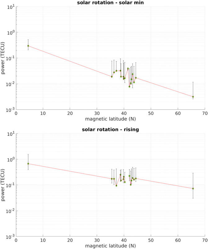
FIGURE 9. Periodogram amplitudes as a function of magnetic latitude for the solar rotation signal during solar minimum (top) and rising phase (bottom). Error bars are calculated from 360-day sub-intervals of each solar phase. This broadband signal is intrinsically harder to quantify than the diurnal and annual signals, but regardless exhibits a general trend of aligning with both magnetic latitude and solar activity.
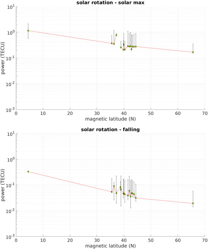
FIGURE 10. Periodogram amplitudes as a function of magnetic latitude for the solar rotation signal during solar maximum (top) and falling phase (bottom). Error bars are calculated from 360-day sub-intervals.
The strong diurnal signal of ionospheric TEC is mainly due to Earth’s rotation. At mid-latitudes, the amplitude of this signal, in addition to the seasonal and solar rotation frequencies, were found to vary on a scale of a hundred to a few hundreds of kilometers. In order to build a predictive capacity for regional-scale TEC at middle-latitudes, which is important at locations such as the Space Coast of Florida or near large airports, it is therefore necessary that whatever model employed be able to reproduce these spectral responses. Without a good characterization of the strong diurnal signal there is no way to predict the strong gradients of TEC which can develop over the Southeastern United States Foster and Rideout. (2007).
Compared to the higher latitude station in Alaska and the lower latitude station in Brazil, the deviation from expected diurnal amplitude (i.e., a straight line fit with respect to magnetic latitude) at mid-latitudes is of the order of a few TECU for each phase of the solar cycle. The number and amplitudes of the diurnal harmonic signals indicate the daily variation is not a perfect sine wave but partially a square wave. This is due to the fact that the night-time recombination rate falls until it reaches the residual ionoziation rate from cosmic rays, defining the trough of a square wave. Our results show that the shape of the diurnal signal varies from station to station and throughout the different phases of the solar cycle. In addition, some stations suggest a significant influence from a twice-daily driver. A key result from the analysis of the diurnal harmonics is that in Alaska the ratio of fundamental and first harmonic amplitudes is constant throughout the solar cycle, while at middle and low latitudes the amplitude ratios have a correspondence with solar activity. Although this could have been expected because the ionospheric drivers are different at those magnetic latitudes, this is the first study to systematically characterize mid-latitude variations of TEC spectral amplitudes for a cluster of observatories with appropriate separation to resolve meso-scale structures.
Based on a ratio of amplitudes that fluctuate around 1 with time, we find that the annual and semi-annual drivers of ionospheric TEC exhibit a competing dominance that varies from station-to-station at mid-latitudes. Olwendo et al. (2016) explain that during equinoxes the sub-solar point is near the equator, where the eastward electric field is often larger, and this intensifies the fountain effect which controls ionization levels at the equator. Near solstices, the subsolar point moves to higher latitudes, and the fountain is expected to wane at the equator. The peak of ionization occurring when solar radiation hits the ionosphere most perpendicularly throughout the year would be at the summer solstice in high latitudes and at the equinoxes at the equator. Therefore, at mid-latitudes we expect the source of strong annual and semi-annual drivers to be a competition of these two effects. In Alaska and Brazil the ratio can approach but always remains greater than 1, indicating the competition of processes plays out less dramatically than at mid-latitudes, i.e. ionosphere TEC is more strongly controlled by a single process.
The mid-latitude meso-scale station-to-station variations of spectral amplitudes (which represent meso-scale spatial structures) and their ratios results from the complex interaction of solar wind-magnetosphere-ionosphere as well as the neutral atmosphere. This interaction can be a source of ionospheric structure for both short (1–10 s of hours) and longer (months to years) time scales. This is further complicated by the fact that the magnetospheric state is determined by instantaneous as well as the time-history of solar wind conditions Lavraud et al. (2006); Borovsky and Valdivia. (2018). It is also the case that space climate is coupled to the neutral atmosphere climate. For instance, transequatorial winds can change the recombination rate by lifting the ionosphere on either side of the equator (Olwendo et al., 2016). The neutral composition has also been shown to have effects on ionospheric storms (Liou et al., 2005). The meso-scale structure of ground conductivity may also play a role in the ionospheric response. The ground conductivities between the different mid-latitude stations in this study vary between 1 and 8 millimhos/meter. Although the more important factor may be proximity to the ocean, where conductivity is close to 5,000 millimhos/meter. However we have not attempted to classify any of these specific effects in this study, only to characterize what are the sum total sinuosoidal responses of the ionosphere due to the combination of driving forces. In this way, it may not be necessary for a predictive model to include the physics of the many competing affects that drive regular TEC oscillations in the ionosphere, just the observed spectral amplitudes. It is also worth noting that for the solar rotation signal a predictive model would benefit from additional information beyond the spectral amplitude, such as the number of sunspots on the solar disc, for example.
Figures, tables, and images will be published under a Creative Commons CC-BY licence and permission must be obtained for use of copyrighted material from other sources (including re-published/adapted/modified/partial figures and images from the internet). It is the responsibility of the authors to acquire the licenses, to follow any citation instructions requested by third-party rights holders, and cover any supplementary charges.
Publicly available datasets were analyzed in this study. This data can be found here: National Geodetic Survey https://geodesy.noaa.gov/CORS/.
BB wrote the manuscript and advised student RC on the data analysis. RC analyzed the data and produced Figures. KN provided funding and help revising the manuscript. XM provided the concept idea for this paper and helped revising the manuscript. SD provided expertise on ionospheric physics.
Support for this work comes from Embry-Riddle internal research funding from the Center for Space and Atmospheric Research (CSAR).
Special thanks to Gopi Seemala for helpful discussions and providing the TEC calculation routines.
The authors declare that the research was conducted in the absence of any commercial or financial relationships that could be construed as a potential conflict of interest.
All claims expressed in this article are solely those of the authors and do not necessarily represent those of their affiliated organizations, or those of the publisher, the editors and the reviewers. Any product that may be evaluated in this article, or claim that may be made by its manufacturer, is not guaranteed or endorsed by the publisher.
Aa, E., Zou, S., Ridley, A., Zhang, S., Coster, A. J., Erickson, P. J., et al. (2019). Merging of storm time midlatitude traveling ionospheric disturbances and equatorial plasma bubbles. Space Weather. 17, 285–298. doi:10.1029/2018SW002101
Afraimovich, E., Astafyeva, E., Oinats, A., Yasyukevich, Y., and Zhivetiev, I. (2008). Global electron content: A new conception to track solar activity. Ann. Geophys. 42, 335–344. doi:10.5194/angeo-26-335-2008
Akinyemi, G. A., Kolawole, L. B., Willoughby, A. A., Dairo, O. F., Abdulrahim, R. B., and Rabiu, A. B. (2021). Variability of GPS-derived ionospheric TEC over Nigeria during a year of low solar activity. Can. J. Phys. 99, 490–495. doi:10.1139/cjp-2020-0113
Amiri-Simkooei, A., and Asgari, J. (2011). Harmonic analysis of total electron contents time series: Methodology and results. GPS Solut. 16, 77–88. doi:10.1007/s10291-011-0208-x
Arikan, F., Nayir, H., Sezen, U., and Arikan, O. (2008). Estimation of single station interfrequency receiver bias using gps-tec. Radio Sci. 43. doi:10.1029/2007RS003785
Borovsky, J. E., and Valdivia, J. A. (2018). The Earth’s magnetosphere: A systems science overview and assessment. Surv. Geophys. 39, 817–859. doi:10.1007/s10712-018-9487-x
Cai, C. (2007). Monitoring seasonal variations of ionospheric tec using gps measurements. Geo-Spatial Inf. Sci. 10, 96–99. doi:10.1007/s11806-007-0034-z
Chauhan, V., Singh, O., and Singh, B. (2011). Diurnal and seasonal variation of gps-tec during a low solar activity period as observed at a low latitude station agra. Indian J. Radio Space Phys. 40, 26–36.
Cheng, Z., and Cummer, S. A. (2005). Broadband vlf measurements of lightning-induced ionospheric perturbations. Geophys. Res. Lett. 32, L08804. doi:10.1029/2004GL022187
Davies, K., Degenhardt, W., Hartmann, G., and Leitinger, R. (1980). Comparison of total electron content measurements made with the ats-6 radio beacon over the u.s. and Europe. J. Atmos. Terr. Phys. 42, 411–416. doi:10.1016/0021-9169(80)90051-3
Elemo, E., Ehigiator, M., and Ehigiator-Irughe, R. (2018). Seasonal variations of the vertical total electron content (vtec) of the ionosphere at the gnss cor station (seerl) uniben and three other cors stations in Nigeria. Nig. J. Tech. 37, 286–293. doi:10.4314/njt.v37i2.1
Foster, J., and Rideout, W. (2007). Storm enhanced density: Magnetic conjugacy effects. Ann. Geophys. 25, 1791–1799. doi:10.5194/angeo-25-1791-2007
Foster, J. C., Zou, S., Heelis, R. A., and Erickson, P. J. (2021). “Ionospheric storm-enhanced density plumes,” in Ionosphere Dynamics and Applications. Editor C. Huang, G. Lu, Y. Zhang, and L. J. Paxton (Washington, D.C., United States: American Geophysical Union). Chap. 6. doi:10.1002/9781119815617
Guo, J., Li, W., Liu, X., Kong, Q., Zhao, C., and Guo, B. (2015). Temporal-spatial variation of global GPS-derived total electron content, 1999-2013. PLoS ONE 10, e0133378. doi:10.1371/journal.pone.0133378
Hines, C. O. (1959). An interpretation of certain ionospheric motions in terms of atmospheric waves. J. Geophys. Res. 64, 2210–2211. doi:10.1029/JZ064i012p02210
Hines, C. O. (1960). Internal atmospheric gravity waves at ionospheric heights. Can. J. Phys. 38, 1441–1481. doi:10.1139/p60-150
Huang, Z., and Roussel-Dupré, R. (2005). Total electron content (tec) variability at los alamos, New Mexico: A comparative study: Forte-derived tec analysis. Radio Sci. 40. doi:10.1029/2004RS003202
Hunsucker, R. D. (1982). Atmospheric gravity waves generated in the high-latitude ionosphere: A review. Rev. Geophys. 20, 293–315. doi:10.1029/RG020i002p00293
Kelley, M. C. (1989a). “Chapter 4 - equatorial plasma instabilities,” in The Earth’s ionosphere. Editor M. C. Kelley (Academic Press), 113–185. doi:10.1016/B978-0-12-404013-7.50009-5
Kelley, M. C. (1989b). “Chapter 8 - instabilities and structure in the high-latitude ionosphere,” in The Earth’s ionosphere. Editor M. C. Kelley (Academic Press), 345–423. doi:10.1016/B978-0-12-404013-7.50013-7
Lavraud, B., Thomsen, M. F., Borovsky, J. E., Denton, M. H., and Pulkkinen, T. I. (2006). Magnetosphere preconditioning under northward imf: Evidence from the study of coronal mass ejection and corotating interaction region geoeffectiveness. J. Geophys. Res. 111, A09208. doi:10.1029/2005JA011566
Lay, E. H., Shao, X.-M., Kendrick, A. K., and Carrano, C. S. (2015). Ionospheric acoustic and gravity waves associated with midlatitude thunderstorms. J. Geophys. Res. Space Phys. 120, 6010–6020. doi:10.1002/2015JA021334
Lay, E. H., Parker, P. A., Light, M., Carrano, C. S., Debchoudhury, S., and Haaser, R. A. (2018). Midlatitude ionospheric irregularity spectral density as determined by ground-based gps receiver networks. J. Geophys. Res. Space Phys. 123, 5055–5067. doi:10.1029/2018JA025364
Liou, K., Newell, P., Anderson, B., Zanetti, L., and Meng, C.-I. (2005). Neutral composition effects on ionospheric storms at middle and low latitudes. J. Geophys. Res. 110, A05309. doi:10.1029/2004JA010840
Liu, J., Chen, R., Wang, Z., An, J., and Hyyppä, J. (2014). Long-term prediction of the arctic ionospheric TEC based on time-varying periodograms. PLoS ONE 9, e111497. doi:10.1371/journal.pone.0111497
Lomb, N. R. (1976). Least-squares frequency analysis of unequally spaced data. Astrophys. Space Sci. 39, 447–462. doi:10.1007/BF00648343
Ma, G., and Maruyama, T. (2003). Derivation of tec and estimation of instrumental biases from geonet in Japan. Ann. Geophys. 21, 2083–2093. doi:10.5194/angeo-21-2083-2003
Oberheide, J., Hagan, M., Richmond, A., and Forbes, J. (2015). “Dynamical meteorology — Atmospheric tides,” in Encyclopedia of atmospheric Sciences. Editors G. R. North, J. Pyle, and F. Zhang. Second edition edn (Oxford: Academic Press), 287–297. doi:10.1016/B978-0-12-382225-3.00409-6
Ogwala, A., Somoye, E. O., Ogunmodimu, O., Adeniji-Adele, R. A., Onori, E. O., and Oyedokun, O. (2019). Diurnal, seasonal and solar cycle variation in total electron content and comparison with iri-2016 model at birnin kebbi. Ann. Geophys. 37, 775–789. doi:10.5194/angeo-37-775-2019
Olwendo, O., Baki, P., Mito, C., and Doherty, P. (2012). Characterization of ionospheric gps total electron content (gps–tec) in low latitude zone over the kenyan region during a very low solar activity phase. J. Atmos. Solar-Terrestrial Phys. 84-85, 52–61. doi:10.1016/j.jastp.2012.06.003
Olwendo, O. J., Yamazaki, Y., Cilliers, P. J., Baki, P., and Doherty, P. (2016). A study on the variability of ionospheric total electron content over the east african low-latitude region and storm time ionospheric variations. Radio Sci. 51, 1503–1518. doi:10.1002/2015RS005785
Perevalova, N., Polyakova, A., and Zalizovski, A. (2010). Diurnal variations of the total electron content under quiet helio-geomagnetic conditions. J. Atmos. Solar-Terrestrial Phys. 72, 997–1007. doi:10.1016/j.jastp.2010.05.014
Perkins, F. (1973). Spread f and ionospheric currents. J. Geophys. Res. 78, 218–226. doi:10.1029/JA078i001p00218
Sardón, E., and Zarraoa, N. (1997). Estimation of total electron content using gps data: How stable are the differential satellite and receiver instrumental biases? Radio Sci. 32, 1899–1910. doi:10.1029/97RS01457
Sardón, E., Rius, A., and Zarraoa, N. (1994). Estimation of the transmitter and receiver differential biases and the ionospheric total electron content from global positioning system observations. Radio Sci. 29, 577–586. doi:10.1029/94RS00449
Seemala, G. K., and Valladares, C. E. (2011). Statistics of total electron content depletions observed over the south American continent for the year 2008. Radio Sci. 46, RS5019. doi:10.1029/2011RS004722
Tariku, Y. A. (2015). Patterns of GPS-TEC variation over low-latitude regions (African sector) during the deep solar minimum (2008 to 2009) and solar maximum (2012 to 2013) phases. Earth, Planets, Space 67, 35. doi:10.1186/s40623-015-0206-2
Valladares, C. E., Villalobos, J., Hei, M. A., Sheehan, R., Basu, S., MacKenzie, E., et al. (2009). Simultaneous observation of traveling ionospheric disturbances in the northern and southern hemispheres. Ann. Geophys. 27, 1501–1508. doi:10.5194/angeo-27-1501-2009
VanderPlas, J. T. (2018). Understanding the lomb–scargle periodogram. Astrophys. J. Suppl. Ser. 236, 16. doi:10.3847/1538-4365/aab766
Webber, W. (1962). The production of free electrons in the ionospheric d layer by solar and galactic cosmic rays and the resultant absorption of radio waves. J. Geophys. Res. 67, 5091–5106. doi:10.1029/JZ067i013p05091
Woodman, R. F., and La Hoz, C. (1976). Radar observations of F region equatorial irregularities. J. Geophys. Res. 81, 5447–5466. doi:10.1029/JA081i031p05447
Xingliang, H., Yuan, Y., Ou, J., Wen, D., and Xiaowen, L. (2005). The diurnal variations, semiannual and winter anomalies of the ionospheric TEC based on GPS date in China. Prog. Nat. Sci. 15, 56–60. doi:10.1080/10020070512331341770
Keywords: ionosphere, total electron content, mid-latitude, global positioning system, meso-scale structure
Citation: Burkholder BL, Cuellar R, Nykyri K, Ma X and Debchoudhury S (2022) A regional classification of time spectral amplitudes in total electron content: Southeastern United States during solar cycle 24. Front. Astron. Space Sci. 9:1040082. doi: 10.3389/fspas.2022.1040082
Received: 08 September 2022; Accepted: 08 November 2022;
Published: 24 November 2022.
Edited by:
Andrés Calabia, Polytechnic University of Madrid, SpainReviewed by:
Sampad Kumar Panda, K. L. University, IndiaCopyright © 2022 Burkholder, Cuellar, Nykyri, Ma and Debchoudhury. This is an open-access article distributed under the terms of the Creative Commons Attribution License (CC BY). The use, distribution or reproduction in other forums is permitted, provided the original author(s) and the copyright owner(s) are credited and that the original publication in this journal is cited, in accordance with accepted academic practice. No use, distribution or reproduction is permitted which does not comply with these terms.
*Correspondence: B. L. Burkholder, YmxidXJraG9sZGVyQGFsYXNrYS5lZHU=
Disclaimer: All claims expressed in this article are solely those of the authors and do not necessarily represent those of their affiliated organizations, or those of the publisher, the editors and the reviewers. Any product that may be evaluated in this article or claim that may be made by its manufacturer is not guaranteed or endorsed by the publisher.
Research integrity at Frontiers
Learn more about the work of our research integrity team to safeguard the quality of each article we publish.