Ensemble deep learning models for prediction and uncertainty quantification of ground magnetic perturbation

Geomagnetically Induced Currents are one of the most hazardous effects caused by geomagnetic storms. In the past literature, the variations in ground magnetic fields over time, dB/dt were used as a proxy value for GIC. Machine Learning (ML) techniques have emerged as a preferred methodology to predict dB/dt. However, space weather data are highly dynamic in nature, and the data distribution is subject to change over time due to environmental variability. The ML models developed are prone to the uncertainty in the input data and therefore suffer from high variance. In addition, a part of an ML architecture performance is conditional on the variables used to model the system in focus. Therefore, a single algorithm may not generate the required accuracy for a given dataset. In this work, a Bayesian Ensemble ML model has been developed to predict the variations over time of the local ground magnetic horizontal component, dB_H/dt. The Ensemble methodology combines multiple ML models in the prediction process to predict dB_H/dt. Bayesian statistics allow the estimation of model parameters and output as probability distributions, where the variance quantifies the uncertainty. The input data consists of solar-wind data from OmniWeb for the years 2001–2010. The local ground horizontal magnetic components for the corresponding time were calculated using SuperMAG data for the Ottawa ground magnetometer station for the years mentioned above. The years 2011–2015 were selected for model testing, as it encompasses the 5 August 2011 and 17 March 2015 geomagnetic storms. Five different accuracy metrics were considered; namely, Root Mean Squared Error (RMSE), Probability of Detection (POD), Probability of False Detection (PFD), Proportion Correct (PC), and Heidke Skills Score (HSS). The parameter uncertainty of the models is quantified, and the mean predicted dB_H/dt is generated with a 95% credible interval. It can be observed that different models perform better with different datasets and the ensemble model has an accuracy comparable to the models with a relatively strong performance.

1 Introduction

Geomagnetically Induced Currents (GICs) are currents induced in long conductors located on the Earth’s surface and galvanically connected to the ground (Camporeale et al., 2018; Tsurutani and Hajra 2021). GICs are caused by Geomagnetic Disturbances (GMD) or geomagnetic storms (Pirjola 2000). GMDs occur due to the interaction of charged particles from the Sun with the Earth’s magnetosphere (Lakhina and Tsurutani 2016; Salman et al., 2020). GIC has the potential to disrupt electrical devices as transformers on the Earth’s surface (Rajput et al., 2021). For example, one of the strongest recorded GMDs occurred in March 1989, causing a collapse of the power system across the United States, Canada, and Europe. Around 6 million residents in Canada experienced power outage for over 9 h (Gannon et al., 2013; Wang et al., 2020). Therefore GIC is one of the most hazardous threats posed by space weather. With the increasing dependence of humankind on technology, there is a need to analyze and predict GIC to mitigate the risks of damage caused by future geomagnetic storms.

GICs occur because changing magnetic fields induce electric currents in conductors (Oliveira and Ngwira 2017). The magnitude of GIC depends on the environmental conditions and the system it affects (e.g., the topology of an electrical grid) (Liu et al., 2009). There are different methods of measuring GIC. A simple means is attaching a Hall effect probe to a transformer ground (Blake et al., 2018). It would be ideal for measuring GIC to install such sensors in every transformer ground, but such an endeavor could prove expensive and disruptive (Blake et al., 2018). In addition, GICs in the power network can be simulated numerically, but this requires information on the structure and components of the power networks (e.g., transformer types, DC resistances etc.) (Boteler and Pirjola 2014; Blake et al., 2018; Alves Ribeiro et al., 2021). The literature includes studies detailing successful collaboration between power transmission operators and researchers to study GIC (Alves Ribeiro et al., 2021). However, it has been noted that the information on power networks is not frequently made available to the wider scientific community by the power operators (Blake et al., 2018; Pinto et al., 2022). Also, most countries have interconnected power networks with their neighbors. Blake et al. (2018) successfully modeled Ireland’s power network to study GIC. The authors did recognize that this study was possible due to Ireland’s small and relatively isolated network structure. Due to the above reasons, different magnetic indices have been used throughout the literature as a proxy measure for GIC. The scientific community has yet to reach a consensus regarding a particular proxy measure. Trichtchenko and Boteler (2004) studied the correlation of measured peak GIC values with global and local geomagnetic indices. The global index consisted of the 3-h K_p index, and the hourly ranges of the magnetic field variations and hourly peak dB/dt values were considered the local counterpart. They concluded that local geomagnetic indices are a better proxy for describing GIC as its correlation with measured peak GIC values is stronger than the global indices. Several past studies used the change in local ground horizontal magnetic component over time (dB_H/dt), as a proxy measure for GIC (Viljanen 1998; Viljanen et al., 2001; Wintoft 2005; Keesee et al., 2020; Pinto et al., 2022). However, dB_H/dt as a proxy measure is only useful as an indicator of GIC activity (Bailey et al., 2022). The scale of the GIC magnitude is primarily dependent on the horizontal electric field E (Wintoft et al., 2015; Bailey et al., 2022). The mapping between dB_H/dt and E is conditional on the frequency-dependent magnetotelluric transfer function (Chave and Jones 2012). The effectiveness of dB_H/dt as a proxy measure is contingent on the assumptions made about the frequency content (Pulkkinen et al., 2006). For example, Wintoft et al. (2015) made an approximation that the electric field E is directly proportional to dB_H/dt. The authors noted that such an approximation discards ground conductivity which affects E (Cagniard 1953; Viljanen et al., 2014). They observed a linear relationship between the maximum E and dB_H/dt across all the site data considered for their study. This allowed them to express E as the product of dB_H/dt and an empirical coefficient. The coefficient value depends on the test site and on the local ground conductivity model. Therefore, the authors used the assumption of E being directly proportional to dB_H/dt, as a first order approximation for a given site.

Over the years, data relevant to space weather have become readily available. For example, data on solar wind magnetic field and plasma are available to the greater scientific community via OMNIWeb. Another example is SuperMAG, which curates changes in the Earth’s magnetic field from ground-based magnetometers. With the availability of such data, there is an increased interest in Machine Learning (ML) for the purpose of prediction and analysis of space weather phenomena. In the past literature studies have been conducted where ML techniques, like Deep Learning (DL), have been used for dB_H/dt prediction. For example, Wang et al. (2020) developed a hybrid model which used two filtering techniques- Wavelet Transform and Short-Time Fourier Transform for feature extraction, and then combined it with a DL architecture for GIC prediction (Wang et al., 2020). The variant of DL architecture they implemented was a Convolutional Neural Network (CNN). Although CNN is primarily used for image classification, it has also been effective in time series forecasting, as it can effectively extract features from the time series data (Lu et al., 2020). A drawback of CNN is that it is not recurrent, i.e., it does not retain the memory of previous time-series patterns. Instead, it can only train based on the data the model inputs at a particular time step. As correlations exist between observations in a time series data (autocorrelation), a standard CNN would treat all observations as independent, causing misleading results.

Recurrent Neural Network (RNN) architectures can account for sequential dependencies in a time series data. Unlike traditional Neural Networks (NN), a standard RNN consists of a feedback loop. The loop feeds information to the RNN from the previous time step to the current time step. However, RNNs in their standard form tend to suffer from a “long-term dependency” problem, i.e., as the gaps between consecutive information grow, RNNs become unable to connect the information. A special kind of RNN called Long Short Term Memory (LSTM) networks have been specially designed in the past literature to tackle the issue of “long-term dependency” (Manaswi 2018; Sherstinsky 2020). Within the context of dB_H/dt prediction, a comparative study was carried out where a feed-forward Neural Network and an LSTM Neural Network (Keesee et al., 2020) used to predict the East and North components of the ground magnetic field. The magnetic components are then used to derive the dB_H/dt.

A part of an ML architecture performance is conditional on the variables used to model the system in focus (Siddique et al., 2022). Therefore, the accuracy of a model architecture varies depending on the problem at hand. In recent years, ensemble ML has gained popularity within the scientific community for time series and regression forecasting. The ensemble methodology combines multiple ML models in the prediction process to obtain better generalization and performance (Murray 2018). Different approaches exist to implement the ensemble methodology. The basic approach can be grouped into either one of two categories- 1) different model architectures have been implemented, or 2) the same model architecture is used with different parameter estimations, using a different subset of training data. The predictions from each unit model are then combined using a weighted average, or the best model result is selected using a voting mechanism. Because of this, ensemble forecast models have been used by both the ML and space science communities. For example, Murray (2018), highlights the importance of using ensemble techniques in space weather forecasting. Mays et al. (2015) implemented the first ensemble prediction system for CME propagation in a real-time prediction. Although, their ensemble approach is based on the WSA-ENLIL + cone model, a simulation-based technique. Guerra et al. (2015) used a linear combination of probabilistic models to forecast solar flares. They observed that the linear combination improves the overall probabilistic prediction for certain values of decision thresholds.

A critical challenge for most ML techniques is dealing with imprecise or incomplete information Hariri et al. (2019). For example, the OMNI dataset contains approximately 20% of missing data distributed through the years (Keesee et al., 2020). In addition to missing data, the space weather data are subject to stochasticity due to environmental variability. Also, historical occurrences of intense geomagnetic storms are scarce (Salman et al., 2018). Given that the ML models are trained using these datasets, the model parameter estimates and output tends to suffer from high variance and uncertainty (Ayyub and Klir 2006; Siddique et al., 2022). Even with the implemented models having low error during laboratory testing, these predictions, due to their inherent uncertainty, could fail in a real-world deployment (Siddique et al., 2022). Therefore, in addition to model accuracy, ensuring the reliability of the model results should also be at the forefront. Hence, there is a need to quantify uncertainty, as it is a means through which a confidence interval can be quantified on the model prediction and accuracy.

A key strength of ensemble models is their ability to reduce model prediction uncertainty (Murray 2018). The uncertainty in the model parameters is known as epistemic uncertainty, and it can be reduced with more data and parameter optimization (Siddique and Mahmud 2021). However, the uncertainty inherent in the training dataset itself is known as aleatoric uncertainty (Siddique and Mahmud 2021). Unlike epistemic uncertainty, aleatoric does not diminish with more data. A vital component of an ensemble model is the aggregation technique it uses. In recent years, Bayesian Model Averaging (BMA) has been proposed as a statistical method to aggregate numerical model forecasts (Vrugt et al., 2008). BMA is a form of a probabilistic averaging scheme, and, to the best of our knowledge, it has yet to be used in space weather forecasting research. However, its implementation in other scientific domains like molecular biology and atmospheric weather predictions has exhibited its superiority over the member model forecasts (Raftery et al., 2005; Gosink et al., 2017).

This paper aims to address the gap mentioned above in the literature. Using solar wind and ground magnetometer data, a Bayesian ensemble DL model has been implemented to predict dB_H/dt. The model leverages Bayesian inference to obtain a posterior distribution for the target variable and parameters. The dispersion of the distribution represents the uncertainty. Given a probability distribution, theory in statistics dictates that confidence bound can be applied. Therefore, the implemented model quantifies the parameter and model uncertainty and predicts the dB_H/dt with a 95% credible interval. The purpose of quantifying uncertainty is to ensure reliability in the model’s existing prediction and accuracy (Siddique et al., 2022). In addition, the ensemble methodology reaffirms that the results from the model with the relative best performance are considered with greater weight during the averaging of the final prediction.

The remainder of the paper is arranged in the following manner- Section 2 describes the data set, model variables and gives an overview of the implemented model. Section 3 covers the results obtained from the model, followed by Section 4 discussing the pros and cons of the implemented methodology and gives recommendations for future research. Finally, Section 5 concludes the paper.

2 Methodology

2.1 Data acquisition and model variables

The implemented model was trained and tested using ground magnetic components, interplanetary magnetic field (IMF), and solar wind data. The baseline corrected ground magnetic component data was obtained from SuperMAG, which curates data from ground magnetometers across the world. For this paper, Ottawa (OTT) was the ground magnetometer station selected from SuperMAG. The OTT station has a magnetic latitude of 54.98° N, and the local midnight occurs at 05:00 UT. The solar wind and IMF data were collected from OMNIWeb, managed by NASA’s Space Physics Data Facility (Gjerloev 2012). Linear interpolation was used to address the missing values in both datasets. The input data consists of IMF and solar wind data from OMNIWeb. The input vector $\vec{x}$ contains the IMF components, B_X, B_Y, and B_Z, along with the pressure, temperature, speed, and proton density of the solar wind. The target vector $\vec{y}$, represents the change in local ground horizontal magnetic component over time (dB_H/dt). The dB_H/dt values are derived using the B_N and B_E, ground magnetic component data from SuperMAG. The derivation of dB_H/dt is shown in Eq-1 as the resultant value of B_N and B_E ground magnetic component, where the derivatives are approximated by first differences of B_N and B_E over a time interval of 1 min. For this study, the years 2001–2010 were used for model training, and the years 2011–2015 were used for testing. The years 2011 and 2015 were specifically chosen for testing because of the 5 August 2011 and 17 March 2015 geostorms (Pulkkinen et al., 2013; Welling et al., 2018). The training dataset was further split, where a proportion of 20% of the data was used for validation during model training.

$\frac{d{B}_H}{dt}=\sqrt{{\left(\frac{d{B}_N}{dt}\right)}^2+{\left(\frac{d{B}_E}{dt}\right)}^2}(1)$

2.2 Model overview

The Bayesian ensemble DL model implemented in this paper consisted of three separate unit models, namely- Bayesian Neural Network (BNN), Bayesian Convolutional Neural Network (Bayesian CNN), and Bayesian Long Short Term Memory (Bayesian LSTM) network. The three unit models have been distinctly implemented in past studies to predict ground magnetic perturbations using solar wind data, using a dataset similar to this current work (Keesee et al., 2020, Pinto et al., 2022). Therefore, the unit models were chosen to explain and validate any form of improvement or limitation of the ensemble methodology. Finally, the individual predictions from each model are combined using a weighted average scheme called Bayesian Model Averaging (BMA) to derive the final model result. An overview of the implemented Bayesian ensemble DL methodology is illustrated in Figure 1.

FIGURE 1

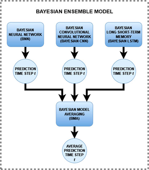
FIGURE 1. Bayesian ensemble model overview.

2.2.1 Bayesian neural network

Bayesian Neural Network (BNN) architecture is the Bayesian counterpart of a traditional feed-forward Artificial Neural Network (ANN) (Mullachery et al., 2018; Jospin et al., 2022; Siddique et al., 2022). The parameters in an ANN are the weights that connect the neurons between two layers. These weights and the final model prediction by an ANN are quantified as point estimates. In contrast, due to the probabilistic nature of a BNN model, both the weight parameters and the model output are derived as a posterior probability distribution (Fortuin et al., 2021; Siddique and Mahmud 2021). BNN leverages Bayesian inference which dictates that the posterior probability is proportional to the product of the likelihood function and the prior probability (Eq. 2) (Hennig et al., 2015; Siddique and Mahmud 2021; Siddique et al., 2022). The BNN model is expressed as p (y|x, D), where y, x, and D, represents the target variable, input variable, and dataset, respectively. The measure of dispersion of the posterior weight distributions p (w|D), and the posterior predictive distribution p (y|x, D), is a quantification of the parameter and output uncertainty, respectively (Tran et al., 2019; Siddique and Mahmud 2021). The output uncertainty is a combination of both epistemic and aleatoric uncertainty (Yao et al., 2019; Siddique et al., 2022). Mathematically, p (y|x, D) can be formulated as shown in Eq. 3 (Siddique and Mahmud 2021). The likelihood function is exhibited in Eq. 4, where $D=\{\vec{x},\vec{y}\}$, represents the training dataset. The negative of the log-likelihood function is maximized to obtain the maximum likelihood estimate (Gómez-Vargas et al., 2021; Siddique and Mahmud 2021). The posterior weight distribution p (w|D) is derived using Variational Inference (VI), where it is approximated using Kullback-Leibler (KL) divergence. Given a variational distribution z (w|D) of Gaussian form, the KL-divergence of r (w—D) and p (w—D) is obtained by minimizing the objective function (shown in Eq. 5) with respect to θ. Given, the mathematical intractability of Eq. 5, it’s negative form called the evidence lower bound (ELBO), is maximized instead (Siddique and Mahmud 2021). The mathematical expression for the ELBO function is shown in Eq. 6. The implemented BNN consisted of 5 hidden layers, with Rectified Linear Unit (ReLU) as the activation function. The loss function, Mean Squared Error (MSE), was minimized using an Adam optimizer. Unlike LSTMs, ANN are incapable of utilizing time history on it’s own. Therefore, the temporal factor was incorporated into the ANN by including a feature vector t that consists of previous time steps, e.g., t − 1, t − 2, etc.

$\mathrm{posterior}\mathrm{probability}\propto \mathrm{likelihood}\times \mathrm{prior}\mathrm{probability}(2)$

$p\left(y|x,D\right)=\int p\left(y|x,w\right)p\left(w|D\right)dw.(3)$

$p\left(D|w\right)=\prod p\left(y|x,w\right).(4)$

$\begin{array}{ll}\hfill \mathbf{KL}\left(r\left(w|\theta \right)\Vert p\left(w|D\right)\right)& =\mathbb{E}\left[\log r\left(w|\theta \right)\right]-\mathbb{E}\left[\log p\left(w\right)\right]\hfill \\ \hfill & -\mathbb{E}\left[\log p\left(D|w\right)\right]+\log p\left(D\right).\hfill \end{array}(5)$

$\mathbf{ELBO}\left(r\right)=\mathbb{E}\left[\log p\left(w\right)\right]+\mathbb{E}\left[\log p\left(D|w\right)\right]-\mathbb{E}\left[\log r\left(w|\theta \right)\right].(6)$

2.2.2 Bayesian convolutional neural network

The second unit model in the ensemble is the Bayesian convolutional neural network (Bayesian CNN). A CNN has an architecture similar to a feed-forward ANN. The difference lies as three additional layers exist between the input and hidden layers (O’Shea and Nash 2015). The first of these layers is called a convolutional layer, which acts as a feature extraction method (Gu et al., 2018). The second layer is the pooling layer, which reduces the size of the feature map from the convolutional layer by filtering the most relevant information (Sun et al., 2017). The last of these three layers is the fully connected layer which flattens the reduced feature map into a column vector, which is then forwarded to the hidden layers (Siddique et al., 2022). A Bayesian CNN consists of a variational distribution as its weight parameters (Gal and Ghahramani 2015; Shridhar et al., 2019). The posterior weight distribution is derived using VI, as discussed in Section 2.2.1. The implemented model consisted of 3 hidden layers. It uses ReLU as the activation function and MSE as the loss function. The loss function is minimized using the Adam optimizer. Since CNN reads in the input matrix all at once, the historic temporal factor was not explicitly given as an input.

2.2.3 Bayesian Long Short Term Memory

The Long Short Term Memory (LSTM) is a variant of recurrent neural network (RNN) (Song et al., 2017). A traditional feed-forward NN is useful for dealing with data independent of each other. RNN differs from a feed-forward NN as they consist of an extra dimension of “memory” that aids in storing information from the previous state to generate the output for the next state in a sequence (DiPietro and Hager 2020). This makes RNNs suitable for dealing with time series prediction. As mentioned in Section 1, RNNs suffer from a “long-term dependency” problem; as the gap in the stored information sequence grows, it is incapable of connecting the information (Sherstinsky 2020). LSTMs address this “long-term dependency” issue. A typical RNN has repeating chain-like modules of NN. A single module takes the previous cell state C_t−1 and the data at current time step x_t as inputs and passes it through a single tanh layer to store the current cell state information C_t, as h_t. LSTM has a similar repeating structure, but in addition to the tanh layer, it consists of three additional sigmoid layers and five pointwise operators, namely, three for multiplication, one for addition, and one for tanh operation. In a cell, the stored information from the previous cell h_t−1 and the current data x_t goes through each of the four layers. The first sigmoid layer produces f_t, the second sigmoid generates i_t, and the last one gives o_t. The tanh layer gives the candidate state ${\widehat{C}}_t$ as output. The outputs of the layers, f_t, i_t, and ${\widehat{C}}_t$ combines with the previous cell state, C_t−1 through pointwise operations of multiplications and additions, to generate the current cell state C_t. A tanh operation is performed on C_t along with a pointwise multiplication of o_t to store the information as h_t. Both C_t and h_t are then passed on to the next cell. The mathematical operations described thus far is exhibited in Eqs 7, 8, 9, 10, 11, 12. The final output from the LSTM gets passed to a Dense layer, which maps all the predicted outputs $\widehat{y}$ to the output layer. In Eqs 7, 8, 9, 10, W_o and b_o represents the weights and biases. Given that the implemented model in the paper is Bayesian, the weights are a variational posterior distribution, which is derived by using VI described in Section 2.2.1.

$f_t=\sigma \left(W_f\left[h_{t-1},x_t\right]+b_f\right)(7)$

$i_t=\sigma \left(W_i\left[h_{t-1},x_t\right]+b_i\right)(8)$

$o_t=\sigma \left(W_o\left[h_{t-1},x_t\right]+b_o\right)(9)$

${\widehat{C}}_t=\tanh \left(W_c\left[h_{t-1},x_t\right]+b_c\right)(10)$

$C_t=f_t{C}_{t-1}+i_t{\widehat{C}}_t(11)$

$h_t=o_t\tanh \left(C_t\right)(12)$

2.2.4 Bayesian model averaging

As mentioned above, the ensemble methodology involves the combination of results from multiple models using a form of voting or average scheme. Given our Bayesian approach, the output from the unit models is in the form of a posterior probability distribution instead of point estimates. In order to combine the posterior distributions from each model, the past literature suggests Bayesian Model Averaging (BMA) (Hoeting et al., 1999; Yao et al., 2018). In BMA, the results are combined by taking a weighted average of the different model results, and the weights are the marginal posterior probability (Yao et al., 2018). This ensures that the aggregation step is performed based on probability as well, making the implemented ensemble methodology an end-to-end probabilistic approach. If $\vec{y}$ = y₁, y₂, … y_n are the set of observed data, and $\vec{M}$ = M₁, M₂, ..M_k are the set of unit models in the ensemble, then the posterior distribution of the combined result, $\widehat{y}$ is $p(\widehat{y}|\vec{y})$ and the mathematical formulation is shown in Eq. 13. Each model is weighed by it’s posterior probability distribution, $p(M_k|\vec{y})$, as exhibited in Eq. 14. The posterior probability distribution depends on the marginal likelihood of each model, $p(\vec{y}|M_k)$, which is illustrated in Eq. 15.

$p\left(\widehat{y}|\vec{y}\right)=\sum _{k=1}^{K}p\left(\widehat{y}|M_k,\vec{y}\right)p\left(M_k|\vec{y}\right)(13)$

$p\left(M_k|\vec{y}\right)=\frac{p\left(\vec{y}|M_k\right)p\left(M_k\right)}{{\sum }_{k=1}^{K}p\left(\vec{y}|M_k\right)p\left(M_k\right)}(14)$

$p\left(\vec{y}|M_k\right)=\int p\left(\vec{y}|{\theta }_k,M_k\right)p\left({\theta }_k|M_k\right)d{\theta }_k.(15)$

3 Results

The implemented models use Bayesian statistics to derive the weight parameters as a posterior probability distribution. Figure 2 shows an instance of posterior weight distribution for each unit model obtained during training. Each weight distribution is labeled with the mean and variance, where the variance quantifies the model parameter uncertainty. A credible interval was placed to ensure the robustness of the parameter estimates. Parameter values that lie between the 95% Highest Density Interval (HDI) were taken forward for the next iteration of the model training. An HDI is the smallest possible interpretation of the credible bound. A narrow credible interval means low distribution variance; therefore, HDI is the minimum dimension of a credible interval. With each training iteration, the variance of the posterior weight distribution is expected to decrease, leading to a reduction in the level of epistemic uncertainty.

FIGURE 2

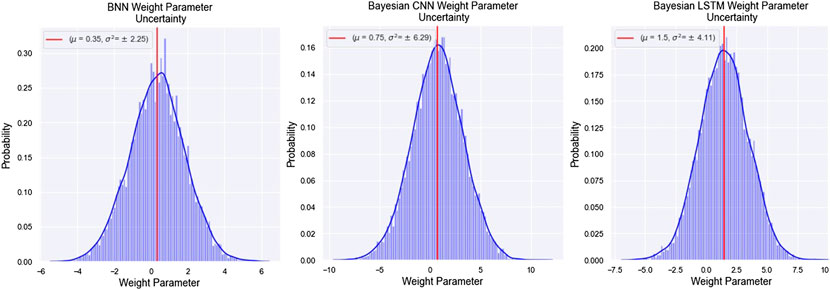
FIGURE 2. Instances of Posterior Weight Distribution For The Three Unit Models- BNN, Bayesian CNN, and Bayesian LSTM. Each Distribution is Labelled With Their Respective Mean and Variance.

As mentioned in the previous section, the data from the 5 August 2011 and 17 March 2015 storms were used for testing the trained unit and ensemble model. The storms were selected in accordance with the recommendations from the Pulkkinen-Welling validation set for ground magnetic perturbations (Pulkkinen et al., 2013; Welling et al., 2018). The storms also correspond to two distinct solar cycle characteristics, with the 2011 storm representing a solar cycle maximum and the 2015 storm characterizing the opposite. Figure 3 illustrates the predicted mean dB_H/dt along with 95% credible interval bound for the storms mentioned above. The ground truth of dB_H/dt for each storm was included for comparison. The figure only shows the first 150 min of the storm for better visual details and exhibition of the prediction uncertainty. The supplementary material includes the graphs containing the predicted and observed storm data over 24 h (1,440 min). An arbitrary predicted mean dB_H/dt has been highlighted in both the figures, along with its corresponding upper and lower bound. This is to display that each time step, the ensemble model gives a prediction in the form of (μ ± 2σ), where μ is the predicted mean dB_H/dt, and σ is the standard deviation representing the level of prediction uncertainty. This standard deviation is a combination of aleatoric and epistemic uncertainty, as mentioned in Section 1.

FIGURE 3

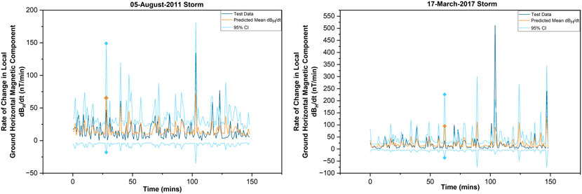
FIGURE 3. The predicted mean rate of local horizontal magnetic component (dB_H/dt), with corresponding variance at each time step, for the 05 August 2011 and 17 March 2015 storms. In each graph, an arbitrary predicted mean has been highlighted along with its corresponding upper and lower bounds, to exhibit the level of prediction uncertainty at that particular time step. The first 150 min have been shown in this figure for better visual details and exhibition of the prediction uncertainty. The graphs containing the predicted mean and observed dB_H/dt over a time period of 24 h is included in the supplementary material.

To further validate the performances of the models, five distinct metrics were employed; namely, Normalized Root Mean Squared Error (NRMSE), Probability of Detection (POD), Probability of False Detection (PFD), Proportion Correct (PC), and Heidki Skill Score (HSS). NRMSE is a popular metric for evaluating the regression performance of machine learning models (Siddique et al., 2022). It is a measure of the deviation of the predicted value from the observed data. It is calculated as the squared root of the mean squared difference between the observed and predicted value (Eq. 16). The RMSE is normalized as shown in Eq. 17. The range of NRMSE lies between 0 and 1, with 0 representing no error or perfect model performance. The NRMSE results for each model are summarized in Table 1. It can be observed from the table that the models performed better for the 2015 storm compared to the one that occurred in 2011. In the case of the 2011 storm, Bayesian CNN outperformed all the other unit models by a small margin, and the Bayesian LSTM performed the poorest. The NRMSE of the ensemble model is comparable to the Bayesian CNN. This similarity in performance between the Bayesian ensemble and Bayesian CNN model was expected, given that the latter is an ensemble unit. The unit models with relatively better performance will be considered with more significant weight during the Bayesian averaging step. In the case of 2015 data, the performance of the BNN is the strongest among the unit models. It can again be observed that the Bayesian Ensemble model has an NRMSE which is comparable to the unit models with the relatively better performance.

TABLE 1

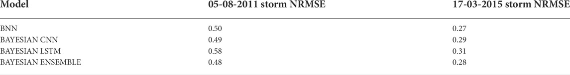
TABLE 1. Normalized root mean squared error (NRMSE) for each of the unit models, and the bayesian ensemble model.

$RMSE=\sqrt{\frac{1}{N}\sum _{i=1}^N{\left(y_i-\widehat{y_i}\right)}^2}(16)$

$NRMSE=\sqrt{\frac{RMSE}{y_{\max }-y_{\min }}}(17)$

The remaining metrics are chosen based on the recommendations from Pulkkinen-Welling for the validation of ground magnetic perturbation forecast (Pulkkinen et al., 2013; Welling et al., 2018). The four metrics are based on binary event analysis, where the observed and predicted time series values are divided into non-overlapping windows consisting of 20 min each. Four thresholds are considered for the analysis, 18 nT/min, 42 nT/min, 66 nT/min, and 90 nT/min. The local maximum dB_H/dt value from both observed and predicted mean is determined for each window. If the observed and predicted mean crosses a given threshold, it is a true positive or a Hit (H). If neither crosses the threshold, there is a true negative (N). If the predicted local maximum crosses but the observed counterpart does not, then there is a false positive (F). In the case where the observed local maximum crosses the threshold whereas the predicted local maximum does not, then there is a false negative (M). The four metrics POD, PFD, PC, and HSS are calculated for each of the four thresholds. POD measures the fraction of observed threshold crossing that was correctly predicted (Pulkkinen et al., 2013), and it is calculated as shown in Eq. 18. POD ranges from 0 to 1, with 1 representing a perfect score. POD is used with PFD, which denotes the number of intervals where the threshold crossings were predicted but did not occur. The mathematical formulation for PFD is exhibited in Eq. 19. PFD also ranges from 0 to 1, but 0 represents the ideal score in this case. The third metric is PC, which measures the proportion of correct prediction and is calculated as illustrated in Eq. 20. PC is of particular interest when calculating HSS. HSS is the proportion of correctly predicted threshold crossings after deducting the crossings due to random chance. The reference model used in calculating the HSS is the PC obtained for random predictions, statistically independent of the observations. The formula for calculating HSS is given in Eq. 21. HSS has a range of − ∞ to 1. A negative HSS indicates that the random predictions are better than the model predictions; 0 indicates that the random and model predictions are the same, that is, the model has no skills; and a positive score means the model predictions are better than random, with 1 corresponding to a perfect score.

$POD=\frac{H}{H+M}(18)$

$PFD=\frac{F}{F+N}(19)$

$PC=\frac{H+N}{H+N+F+M}(20)$

$HSS=\frac{2\left(HN-MF\right)}{\left(H+M\right)\left(M+N\right)+\left(H+F\right)\left(F+N\right)}(21)$

Table 2 summarizes the validation metric scores for each model when tested with the storms mentioned above. The missing values in the table are due to no occurrences of the observed and predicted dB_H/dt crossing the higher thresholds. The overall POD and HSS values show that the models have a better performance with the 2015 storm than with the 2011 storm. This is consistent with the findings from the NRMSE metric above. It can be deduced that not only do the models perform better in predicting point estimates of dB_H/dt, but it is also able to capture the time series trend better and spikes in dB_H/dt for the 2015 storm relative to its 2011 counterpart. In the case of the 2011 storm, the BNN outperforms the other unit models. This is evident in the high POD and PC values and the low PFD values. However, all the models only show a positive HSS score for the first threshold and have skills equal to that of a random reference model for the remaining three thresholds. Even amongst the first threshold, BNN has the highest skill score. In the case of the 2015 storm, the POD and PFD values are comparable.

TABLE 2

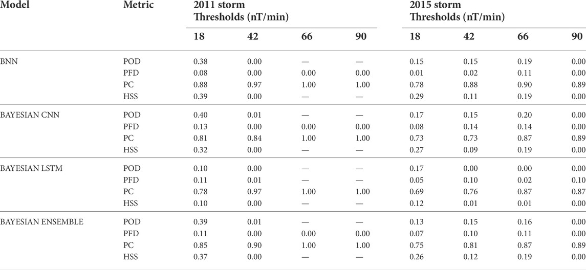
TABLE 2. Validation metrics for the 05 August 2011 and the 17 March 2015 geomagnetic storms using predicted dB_H/dt maximum values for every 20 min time period. The threshold values (18, 42, 66, and 90) have a unit of nT/min.

Regarding HSS, all the unit models have positive skills scores by a small margin for the first three thresholds, with BNN having the highest score among the three. For both storms, the ensemble model has a performance comparable to the performance of the best unit model. This is again consistent with the findings from the NRMSE metric, as the ensemble model considers the best model results with a greater degree of weight. Amongst the four metrics, HSS was the primary metric used for comparison, as has been the case for other studies using a similar dataset (Keesee et al., 2020; Pinto et al., 2022). However, using a single metric can be restrictive as, at times, it can fail to provide deeper insight into the model’s strengths and weakness (Pinto et al., 2022). For example, in the case of HSS (Eq. 21), in case of a weak event, the numerator and denominator could both end up being zero, in which case we would end up with “NaN” values (Pulkkinen et al., 2013). Therefore, other supporting metrics must be incorporated into the study as well.

4 Discussion and future work

The ensemble methodology implemented in this paper exhibits as a result that the performance of different model architectures varies based on the data set used for testing. This is evident from the NRMSE values in Table 1, where the Bayesian CNN had the best performance for the 2011 storm, whereas the BNN had the strongest performance for the 2015 storm. The ensemble nature of the approach ensures that the result from the best model architecture is carried forward towards the final result with greater weight during averaging. In addition, a substantial portion of the training dataset consists of quiet times with low geomagnetic fluctuations, whereas the models were tested against geomagnetic storms, which consist of high fluctuations. This could cause the model outputs to suffer from a degree of biasness. Bayesian statistics allows the models to quantify model uncertainty and predict the output with a confidence interval, thus ensuring reliability in the model’s obtained output, in case there are any biasness. However, there is room for improvement in the implemented approach. The Bayesian nature of the model, especially the Bayesian Averaging step, is computationally expensive. Therefore, in its current form, any attempt at real-time prediction with the existing ensemble model will have significant time lags. This can be addressed by introducing a form of distributed DL. In distributed ML, multiple Graphics Processing Units (GPUs) are employed to speed up the training and testing process. This is achieved by either performing model parallelism or data parallelism. In model parallelism, the model’s different layers into separate GPUs. In data parallelism, the same model versions exist in distinct GPUs, and a different subset of data is run on each version of the model. A similar principle of distributed learning can be applied in ensemble learning, where each unit model is executed on different GPUs, along with the weighted average scheme for the final prediction being performed in a distinct GPU. Depending on the time and space complexity issue at hand, data parallelism can also be applied.

Keesee et al. (2020) used a dataset similar to this study, where they tested a trained ANN and LSTM model against the 2011 and 2015 storms using data set from the Ottawa station. In their work, only the ANN came close to predicting the initial spike of the 2011 storm, whereas both models failed to capture the initial spike for the 2015 storm. However, in our case, the implemented ensemble model was close to capturing the initial spike for both storms. This improvement for the 2015 storm forecast can likely be attributed to the inclusion of the CNN as a unit model of the ensemble. Furthermore, the findings of our LSTM are consistent with the paper mentioned above. The LSTM model generally performed the poorest across both storms in their study. They suggested that the poor performance can likely be attributed to their model implementation. In their LSTM, they did not include the time history of the features, despite it being the strength of such a model. However, the LSTM implemented for our work does consist of the temporal history but still fails to show a marked improvement. Therefore, this paper recommends that different cell structures for LSTM be explored in future research endeavors to determine the best design for forecasting ground magnetic perturbation. Given the black-box nature of DL, researchers have adopted practices to explain how the model maps the inputs features to the outputs (Ras et al., 2022). Therefore, similar practices can be explored when applying DL in future ground magnetic perturbation forecast studies to understand better a model’s performance and how its architecture can be improved to map the problem in focus adequately.

5 Conclusion

This paper developed a Bayesian Ensemble DL model to quantify model uncertainty while predicting dB_H/dt values using solar wind and ground magnetometer data. The ensemble consisted of a BNN, Bayesian CNN, and Bayesian LSTM. A Bayesian weighted average scheme was employed to determine the final prediction with a 95% confidence interval. Five metrics were used to evaluate the model performance: NRMSE, POD, PFD, PC, and HSS. The models were tested against the storm data from 05 August 2011 and 17 March 2015. All the models performed better with the 2015 storm than the one that occurred in 2011. Amongst the unit models, BNN outperformed the others, and the accuracy and skill of the ensemble model are comparable to the BNN. The paper further discusses the implemented approach’s pros and cons and recommends future improvements and research avenues.

Data availability statement

The solar wind, IMF, and Sym-H index data are available from OMNIWeb at https://omniweb.gsfc.nasa.gov, and the ground magnetometer data are available from SuperMAG at http://supermag.jhuapl.edu.

Author contributions

TS was the primary author of the paper, conducted data preparation, model development, and participated in the analysis. MM provided guidance on study concept and design, model development and analysis, interpretation of results, and writing.

Funding

This work was supported by NSF EPSCoR Award OIA-1920965.

Acknowledgments

We thank all members of the MAGICIAN team at UNH and UAF that participated in discussions leading to this article. We thank NASA OMNIweb and SuperMAG for providing organized data access that supported this study.

Conflict of interest

The authors declare that the research was conducted in the absence of any commercial or financial relationships that could be construed as a potential conflict of interest.

Publisher’s note

All claims expressed in this article are solely those of the authors and do not necessarily represent those of their affiliated organizations, or those of the publisher, the editors and the reviewers. Any product that may be evaluated in this article, or claim that may be made by its manufacturer, is not guaranteed or endorsed by the publisher.

References

Alves Ribeiro, J., Pinheiro, F. J. G., and Pais, M. A. (2021). First estimations of geomagnetically induced currents in the south of Portugal. Space weather. 19, e2020SW002546. doi:10.1029/2020sw002546

CrossRef Full Text | Google Scholar

Ayyub, B. M., and Klir, G. J. (2006). Uncertainty modeling and analysis in engineering and the sciences. October. doi:10.1201/9781420011456

CrossRef Full Text | Google Scholar

Bailey, R. L., Leonhardt, R., Möstl, C., Beggan, C., Reiss, M. A., Bhaskar, A., et al. (2022). Forecasting GICs and geoelectric fields from solar wind data using LSTMs: Application in Austria. Space weather. 20. doi:10.1029/2021SW002907

CrossRef Full Text | Google Scholar

Blake, S. P., Gallagher, P. T., Campanyà, J., Hogg, C., Beggan, C. D., Thomson, A. W. P., et al. (2018). A detailed model of the Irish high voltage power network for simulating gics. Space weather. 16, 1770–1783. doi:10.1029/2018SW001926

CrossRef Full Text | Google Scholar

Boteler, D. H., and Pirjola, R. J. (2014). Comparison of methods for modelling geomagnetically induced currents. Ann. Geophys. 32, 1177–1187. doi:10.5194/angeo-32-1177-2014

CrossRef Full Text | Google Scholar

Cagniard, L. (1953). Basic theory of the magneto-telluric method of geophysical prospecting. GEOPHYSICS 18, 605–635. doi:10.1190/1.1437915

CrossRef Full Text | Google Scholar

E. Camporeale, J. R. Johnson, and S. Wing (Editors) (2018). Machine learning techniques for space weather (Amsterdam, Netherlands ; Cambridge, MA: Elsevier). OCLC: on1042806041.

Google Scholar

A. D. Chave, and A. G. Jones (Editors) (2012). The magnetotelluric method: Theory and practice. 1 edn (Cambridge University Press). doi:10.1017/CBO9781139020138

CrossRef Full Text | Google Scholar

DiPietro, R., and Hager, G. D. (2020). “Chapter 21 - deep learning: Rnns and lstm,” in Handbook of medical image computing and computer assisted intervention. The elsevier and MICCAI society book series. Editors S. K. Zhou, D. Rueckert, and G. Fichtinger (Academic Press), 503–519. doi:10.1016/B978-0-12-816176-0.00026-0

CrossRef Full Text | Google Scholar

Fortuin, V., Garriga-Alonso, A., Wenzel, F., Rätsch, G., Turner, R., van der Wilk, M., et al. (2021). Bayesian neural network priors revisited. arXiv preprint arXiv:2102.06571.

Google Scholar

Gal, Y., and Ghahramani, Z. (2015). Bayesian convolutional neural networks with Bernoulli approximate variational inference. arXiv preprint arXiv:1506.02158.

Google Scholar

Gannon, J., Balch, C., and Trichtchenko, L. (2013). “Regional United States electric field and gic hazard impacts,” in AGU fall meeting abstracts, 2013. SM52C–04.

Google Scholar

Gjerloev, J. W. (2012). The SuperMAG data processing technique: Technique. J. Geophys. Res. 117. doi:10.1029/2012JA017683

CrossRef Full Text | Google Scholar

Gómez-Vargas, I., Esquivel, R. M., García-Salcedo, R., and Vázquez, J. A. (2021). “Neural network within a bayesian inference framework,”. Journal of Physics: Conference series (Mexico City, Mexico: IOP Publishing), 1723, 012022.

Google Scholar

Gosink, L. J., Overall, C. C., Reehl, S. M., Whitney, P. D., Mobley, D. L., and Baker, N. A. (2017). Bayesian model averaging for ensemble-based estimates of solvation-free energies. J. Phys. Chem. B 121, 3458–3472. doi:10.1021/acs.jpcb.6b09198

PubMed Abstract | CrossRef Full Text | Google Scholar

Gu, J., Wang, Z., Kuen, J., Ma, L., Shahroudy, A., Shuai, B., et al. (2018). Recent advances in convolutional neural networks. Pattern Recognit. 77, 354–377. doi:10.1016/j.patcog.2017.10.013

CrossRef Full Text | Google Scholar

Guerra, J. A., Pulkkinen, A., and Uritsky, V. M. (2015). Ensemble forecasting of major solar flares: First results: Ensemble forecasting. Space weather. 13, 626–642. doi:10.1002/2015SW001195

CrossRef Full Text | Google Scholar

Hariri, R. H., Fredericks, E. M., and Bowers, K. M. (2019). Uncertainty in big data analytics: Survey, opportunities, and challenges. J. Big Data 6, 44. doi:10.1186/s40537-019-0206-3

CrossRef Full Text | Google Scholar

Hennig, P., Osborne, M. A., and Girolami, M. (2015). Probabilistic numerics and uncertainty in computations. Proc. R. Soc. A 471, 20150142. doi:10.1098/rspa.2015.0142

PubMed Abstract | CrossRef Full Text | Google Scholar

Hoeting, J. A., Madigan, D., Raftery, A. E., and Volinsky, C. T. (1999). Bayesian model averaging: A tutorial (with comments by m. clyde, david draper and ei george, and a rejoinder by the authors. Stat. Sci. 14, 382–417. doi:10.1214/ss/1009212519

CrossRef Full Text | Google Scholar

Jospin, L. V., Laga, H., Boussaid, F., Buntine, W., and Bennamoun, M. (2022). Hands-on bayesian neural networks—A tutorial for deep learning users. IEEE Comput. Intell. Mag. 17, 29–48. doi:10.1109/mci.2022.3155327

CrossRef Full Text | Google Scholar

Keesee, A. M., Pinto, V., Coughlan, M., Lennox, C., Mahmud, M. S., and Connor, H. K. (2020). Comparison of deep learning techniques to model connections between solar wind and ground magnetic perturbations. Front. Astron. Space Sci. 7, 1–8. doi:10.3389/fspas.2020.550874

CrossRef Full Text | Google Scholar

Lakhina, G. S., and Tsurutani, B. T. (2016). Geomagnetic storms: Historical perspective to modern view. Geosci. Lett. 3, 5. doi:10.1186/s40562-016-0037-4

CrossRef Full Text | Google Scholar

Liu, C. M., Liu, L. G., Pirjola, R., and Wang, Z. Z. (2009). Calculation of geomagnetically induced currents in mid- to low-latitude power grids based on the plane wave method: A preliminary case study. Space weather. 7, 1–9. doi:10.1029/2008SW000439

CrossRef Full Text | Google Scholar

Lu, W., Li, J., Li, Y., Sun, A., and Wang, J. (2020). A CNN-LSTM-Based model to forecast stock prices. Complexity 2020, 1–10. doi:10.1155/2020/6622927

CrossRef Full Text | Google Scholar

Manaswi, N. K. (2018). “Rnn and lstm,” in Deep learning with applications using Python (Springer), 115–126.

CrossRef Full Text | Google Scholar

Mays, M. L., Taktakishvili, A., Pulkkinen, A., MacNeice, P. J., Rastätter, L., Odstrcil, D., et al. (2015). Ensemble modeling of CMEs using the WSA–ENLIL+Cone model. Sol. Phys. 290, 1775–1814. doi:10.1007/s11207-015-0692-1

CrossRef Full Text | Google Scholar

Mullachery, V., Khera, A., and Husain, A. (2018). Bayesian neural networks. arXiv preprint arXiv:1801.07710.

Google Scholar

Murray, S. A. (2018). The importance of ensemble techniques for operational space weather forecasting. Space weather. 16, 777–783. doi:10.1029/2018SW001861

CrossRef Full Text | Google Scholar

Oliveira, D. M., and Ngwira, C. M. (2017). Geomagnetically induced currents: Principles. Braz. J. Phys. 47, 552–560. doi:10.1007/s13538-017-0523-y

CrossRef Full Text | Google Scholar

O’Shea, K., and Nash, R. (2015). An introduction to convolutional neural networks. arXiv preprint arXiv:1511.08458.

Google Scholar

Pinto, V. A., Keesee, A. M., Coughlan, M., Mukundan, R., Johnson, J. W., Ngwira, C. M., et al. (2022). Revisiting the ground magnetic field perturbations challenge: A machine learning perspective. Front. Astron. Space Sci. 9, 869740. doi:10.3389/fspas.2022.869740

CrossRef Full Text | Google Scholar

Pirjola, R. (2000). Geomagnetically induced currents during magnetic storms. IEEE Trans. Plasma Sci. IEEE Nucl. Plasma Sci. Soc. 28, 1867–1873. doi:10.1109/27.902215

CrossRef Full Text | Google Scholar

Pulkkinen, A., Viljanen, A., and Pirjola, R. (2006). Estimation of geomagnetically induced current levels from different input data: Gic estimation. Space weather. 4. doi:10.1029/2006SW000229

CrossRef Full Text | Google Scholar

Pulkkinen, A., Rastätter, L., Kuznetsova, M., Singer, H., Balch, C., Weimer, D., et al. (2013). Community-wide validation of geospace model ground magnetic field perturbation predictions to support model transition to operations: Geospace model transition. Space weather. 11, 369–385. doi:10.1002/swe.20056

CrossRef Full Text | Google Scholar

Raftery, A. E., Gneiting, T., Balabdaoui, F., and Polakowski, M. (2005). Using bayesian model averaging to calibrate forecast ensembles. Mon. Weather Rev. 133, 1155–1174. doi:10.1175/MWR2906.1

CrossRef Full Text | Google Scholar

Rajput, V. N., Boteler, D. H., Rana, N., Saiyed, M., Anjana, S., and Shah, M. (2021). Insight into impact of geomagnetically induced currents on power systems: Overview, challenges and mitigation. Electr. Power Syst. Res. 192, 106927. doi:10.1016/j.epsr.2020.106927

CrossRef Full Text | Google Scholar

Ras, G., Xie, N., Van Gerven, M., and Doran, D. (2022). Explainable deep learning: A field guide for the uninitiated. J. Artif. Intell. Res. 73, 329–397. doi:10.1613/jair.1.13200

CrossRef Full Text | Google Scholar

Salman, T. M., Lugaz, N., Farrugia, C. J., Winslow, R. M., Galvin, A. B., and Schwadron, N. A. (2018). Forecasting periods of strong southward magnetic field following interplanetary shocks. Space weather. 16, 2004–2021. doi:10.1029/2018sw002056

CrossRef Full Text | Google Scholar

Salman, T. M., Lugaz, N., Farrugia, C. J., Winslow, R. M., Jian, L. K., and Galvin, A. B. (2020). Properties of the Sheath Regions of Coronal Mass Ejections with or without Shocks from STEREO in situ Observations near 1 au. Astrophys. J. 904, 177. doi:10.3847/1538-4357/abbdf5

CrossRef Full Text | Google Scholar

Sherstinsky, A. (2020). Fundamentals of recurrent neural network (rnn) and long short-term memory (lstm) network. Phys. D. Nonlinear Phenom. 404, 132306. doi:10.1016/j.physd.2019.132306

CrossRef Full Text | Google Scholar

Shridhar, K., Laumann, F., and Liwicki, M. (2019). A comprehensive guide to bayesian convolutional neural network with variational inference. arXiv preprint arXiv:1901.02731.

Google Scholar

Siddique, T., and Mahmud, M. S. (2021). Classification of fnirs data under uncertainty: A bayesian neural network approach.

Google Scholar

Siddique, T., Mahmud, M. S., Keesee, A. M., Ngwira, C. M., and Connor, H. (2022). A survey of uncertainty quantification in machine learning for space weather prediction. Geosciences 12, 27. doi:10.3390/geosciences12010027

CrossRef Full Text | Google Scholar

Song, J., Guo, Z., Gao, L., Liu, W., Zhang, D., and Shen, H. T. (2017). Hierarchical lstm with adjusted temporal attention for video captioning. arXiv preprint arXiv:1706.01231.

Google Scholar

Sun, M., Song, Z., Jiang, X., Pan, J., and Pang, Y. (2017). Learning pooling for convolutional neural network. Neurocomputing 224, 96–104. doi:10.1016/j.neucom.2016.10.049

CrossRef Full Text | Google Scholar

Tran, D., Dusenberry, M., van der Wilk, M., and Hafner, D. (2019). Bayesian layers: A module for neural network uncertainty. Adv. neural Inf. Process. Syst. 32. doi:10.48550/arXiv.1812.03973

CrossRef Full Text | Google Scholar

Trichtchenko, L., Boteler, D., and Boteler, D. (2004). Modeling geomagnetically induced currents using geomagnetic indices and data. IEEE Trans. Plasma Sci. IEEE Nucl. Plasma Sci. Soc. 32, 1459–1467. doi:10.1109/TPS.2004.830993

CrossRef Full Text | Google Scholar

Tsurutani, B. T., and Hajra, R. (2021). The interplanetary and magnetospheric causes of geomagnetically induced currents (gics) > 10 a in the mäntsälä Finland pipeline: 1999 through 2019. J. Space Weather Space Clim. 11, 23. doi:10.1051/swsc/2021001

CrossRef Full Text | Google Scholar

Viljanen, A., Nevanlinna, H., Pajunpää, K., and Pulkkinen, A. (2001). Time derivative of the horizontal geomagnetic field as an activity indicator. Ann. Geophys. 19, 1107–1118. doi:10.5194/angeo-19-1107-2001

CrossRef Full Text | Google Scholar

Viljanen, A., Pirjola, R., Prácser, E., Katkalov, J., and Wik, M. (2014). Geomagnetically induced currents in Europe: Modelled occurrence in a continent-wide power grid. J. Space Weather Space Clim. 4, A09. doi:10.1051/swsc/2014006

CrossRef Full Text | Google Scholar

Viljanen, A. (1998). Relation of geomagnetically induced currents and local geomagnetic variations. IEEE Trans. Power Deliv. 13, 1285–1290. doi:10.1109/61.714497

CrossRef Full Text | Google Scholar

Vrugt, J. A., Diks, C. G. H., and Clark, M. P. (2008). Ensemble Bayesian model averaging using Markov chain Monte Carlo sampling. Environ. Fluid Mech. (Dordr). 8, 579–595. doi:10.1007/s10652-008-9106-3

CrossRef Full Text | Google Scholar

Wang, S., Dehghanian, P., Li, L., and Wang, B. (2020). A machine learning approach to detection of geomagnetically induced currents in power grids. IEEE Trans. Ind. Appl. 56, 1098–1106. doi:10.1109/TIA.2019.2957471

CrossRef Full Text | Google Scholar

Welling, D. T., Ngwira, C. M., Opgenoorth, H., Haiducek, J. D., Savani, N. P., Morley, S. K., et al. (2018). Recommendations for next-generation ground magnetic perturbation validation. Space weather. 16, 1912–1920. doi:10.1029/2018SW002064

CrossRef Full Text | Google Scholar

Wintoft, P. (2005). Study of the solar wind coupling to the time difference horizontal geomagnetic field. Ann. Geophys. 23, 1949–1957. doi:10.5194/angeo-23-1949-2005

CrossRef Full Text | Google Scholar

Wintoft, P., Wik, M., and Viljanen, A. (2015). Solar wind driven empirical forecast models of the time derivative of the ground magnetic field. J. Space Weather Space Clim. 5, A7–P9. doi:10.1051/swsc/2015008

CrossRef Full Text | Google Scholar

Yao, J., Pan, W., Ghosh, S., and Doshi-Velez, F. (2019). Quality of uncertainty quantification for bayesian neural network inference. arXiv preprint arXiv:1906.09686.

Google Scholar

Yao, Y., Vehtari, A., Simpson, D., and Gelman, A. (2018). Using stacking to average bayesian predictive distributions (with discussion). Bayesian Anal. 13, 917–1007. doi:10.1214/17-ba1091

CrossRef Full Text | Google Scholar