 Kiera van der Sande
 Natasha Flyer1,2
 Thomas E. Berger
- 1Department of Applied Mathematics, University of Colorado at Boulder, Boulder, CO, United States
- 2Flyer Research LLC, Boulder, CO, United States
- 3Space Weather Technology, Research and Education Center, University of Colorado at Boulder, Boulder, CO, United States
- 4Department of Aerospace Engineering, University of Colorado at Boulder, Boulder, CO, United States
Supervised Machine Learning (ML) models for solar flare prediction rely on accurate labels for a given input data set, commonly obtained from the GOES/XRS X-ray flare catalog. With increasing interest in utilizing ultraviolet (UV) and extreme ultraviolet (EUV) image data as input to these models, we seek to understand if flaring activity can be defined and quantified using EUV data alone. This would allow us to move away from the GOES single pixel measurement definition of flares and use the same data we use for flare prediction for label creation. In this work, we present a Solar Dynamics Observatory (SDO) Atmospheric Imaging Assembly (AIA)-based flare catalog covering flare of GOES X-ray magnitudes C, M and X from 2010 to 2017. We use active region (AR) cutouts of full disk AIA images to match the corresponding SDO/Helioseismic and Magnetic Imager (HMI) SHARPS (Space weather HMI Active Region Patches) that have been extensively used in ML flare prediction studies, thus allowing for labeling of AR number as well as flare magnitude and timing. Flare start, peak, and end times are defined using a peak-finding algorithm on AIA time series data obtained by summing the intensity across the AIA cutouts. An extremely randomized trees (ERT) regression model is used to map SDO/AIA flare magnitudes to GOES X-ray magnitude, achieving a low-variance regression. We find an accurate overlap on 85% of M/X flares between our resulting AIA catalog and the GOES flare catalog. However, we also discover a number of large flares unrecorded or mislabeled in the GOES catalog.
1 Introduction
There is growing interest in using ultraviolet (UV) and extreme ultraviolet (EUV) images from instruments such as the NASA Solar Dynamics Observatory (SDO) Atmospheric Imaging Assembly (AIA) or the NOAA Geostationary Operational Environment Satellite (GOES) Solar Ultraviolet Imager (SUVI) for prediction of solar magnetic eruptions, as these images may contain more precursor features associated with eruptions than the photospheric magnetic field data that have been primarily used to date. Modern data analytic methods for solar eruption prediction have centered on the use of machine learning (ML) models to derive predictive patterns from the increasing amounts of solar imaging data accumulated over the past several decades , for example, the work of (Qahwaji and Colak, 2007; Bobra and Couvidat, 2015; Barnes et al., 2016; Nishizuka et al., 2017; Jonas et al., 2018; Leka et al., 2019a; Leka et al., 2019b; Park et al., 2020). The most common ML models to date rely on “supervised learning” in which researchers must provide labeled data for training the model. These labels must accurately identify eruptive from non-eruptive states for each image in any given training data set as well as eruptive magnitudes for studies that aim to provide both timing and magnitude predictions.
Solar eruption timing and magnitude are currently defined using measurements of X-ray radiation from the associated “solar flares” measured with the NOAA Geostationary Operational Environment Satellite (GOES) X-ray Sensors (XRS) instrument. GOES XRS measurements are full-disk, “Sun as a star,” spectral irradiance measurements acquired at a 1-s cadence in two wavelength bands: the XRS-A channel from 0.5–4 Å and the XRS-B channel from 1 to 8 Å. Flare magnitude classes of A, B, C, M and X are defined by their peak irradiance in the XRS-B channel1. A key characteristic of GOES/XRS flare identification is that until the recent GOES-R instruments, first launched in 2016, there was no spatial information to locate the eruption site on the disk. Instead, human forecasters used X-ray, UV, and/or EUV imaging observations (typically from the GOES Solar X-ray Imager, SXI, AIA or SUVI) for post-facto identification of the sunspot active region (AR) that generated the eruption, adding potential for error since at least two separate observational systems with a human in the loop are required. In fact, sunspot ARs are identified and numbered based on a third observational data type (solar continuum images), adding yet another source for error in associating an AR number with any given eruption. The GOES-R instruments added the ability to estimate flare locations using a quad-diode sensor rather than the single pixel sensor of previous XRS implementations, however the locations from this system are only accurate for large flares, and the instruments have only been in operation since 2016 (Chamberlin et al., 2009), which was approaching the minimum of activity in Solar Cycle 24 (c.2008–2019).
The GOES X-ray flare catalog2, which has entries from 1975 to the present, is the most extensive record of solar eruptions to date. It includes peak X-ray irradiance, disk location in heliographic coordinates, the associated sunspot AR number, as well as start, peak, and end times for flares from B-magnitude (XRS-B peak irradiance between 10–7 and 10–6 Wm−2) and above. It is one of the most common source of labels for supervised ML model development, but it has compatibility problems when used with ML models that use training data based on images of individual sunspot ARs rather than full-disk data. Specifically, if the training data are individual ARs, it is imperative that the labels derived from the GOES catalog are 1) available for each AR in the training set, and 2) accurate across the entire training set for all flare intensities. ML models are particularly sensitive to training set labelling errors, particularly when studying episodic and impulsive events like solar eruptions in which the training set is inherently highly imbalanced: the high temporal cadence of modern solar telescopes ensures that there are always many more “no flare” labelled images than “flare” labelled images for any predictive time window.
We note that there are additional flare catalogs available. In fact, there is a new GOES database3, which is recommended for use and includes a reprocessed flare summary for data from 2010 to 2020. While this database will be useful for future studies, flare locations are currently only available from 2017 onward, so the summary of flares from 2010 to 2020 based on the GOES-15 satellite only includes flaring timing and magnitude data, not even corresponding ARs. Another commonly used catalog is obtained from the Heliophysics Event Knowledgebase (HEK)4. For this analysis, we compare to the older GOES flare catalog 2, which is known to have errors, allowing us to test the robustness of our AIA-based catalog in detecting those errors. We refer to this event list as the GOES flare catalog for the remainder of this work.
Because of their higher occurrence frequency and the ambiguity inherent in locating smaller flares during periods when multiple ARs are on the disk, many flares at and below C-class lack an associated disk location and/or AR number in the GOES catalog, making these events unusable for ML model training. Even a significant fraction of M-flares lack a disk position or associated AR number in the catalog. In addition, a number of C- and even many M-class flares are assigned to incorrect ARs in the GOES catalog. Cursory investigation has so far identified on the order of 20 cases in which M-class flares are either lacking a disk position and/or AR number, or are assigned to the incorrect AR number in the GOES catalog. We show below that we have also discovered on the order of 50 cases in which M-class flares , as estimated by our AIA-based flare magnitude regression model, are entirely absent from the catalog, some of which may be due to a mismatch in timing between the GOES X-ray measurements and flaring activity in AIA. For our associated ML flare prediction project which relies on training images of flaring and non-flaring ARs from Solar Cycle 24, which was a relatively weak activity cycle, this translates into a potential increase of approximately 15% of images in the training set that should be labelled as “flare” images, which would significantly compromise our model’s predictive skill without correction.
In this study, we explore the possibility of defining and classifying flares using only UV and EUV imaging data of individual ARs, thus producing an internally consistent process for labelling ML training data: since we are already creating AR cutout images as the training data, there is no need to rely on a secondary data source or catalog for event labelling or magnitude classification. In addition, studies of the upper atmospheric impacts of flares show that the majority of ionization above about 100 km in the thermosphere is caused by enhancements in EUV radiation in the 10–300 Å range (Solomon, 2005; Qian et al., 2012). Thus GOES/XRS magnitude alone is often not indicative of the ionospheric impact of major flares. For example, the largest X-ray flare in the GOES catalog (X28.0 on 4-November-2003) had a lesser impact on ionospheric total electron content (TEC) than the significantly smaller X10.0 flare on 14-July-2000 due to a much lower broadband EUV enhancement, possibly related to the limbward disk position of the larger flare (Tsurutani, 2005). Studies have attempted to correlate GOES/XRS 1–8 Å measurements to broadband EUV irradiance (e.g., 13) with limited success. The SDO mission includes the Extreme ultraviolet Variability Experiment (EVE) instrument specifically to address this issue. Having an independent “EUV flare” definition from imaging data may aid both ML model development as well as upper atmospheric ionization studies. The main questions being investigated here are:
• Can we use AIA data to identify solar flares and reliably quantify their magnitudes?
• How well do the resultant EUV flare magnitudes correlate with the historically important GOES X-ray flare magnitudes?
• Can we create a ML-based regression model to predict the flare GOES class from EUV magnitudes?
In Section 2 we describe the SDO/AIA data and pre-processing steps. Section 3 shows the correspondence between flare start and end times defined in UV and EUV images with those listed in the GOES flare catalogs and verifies prior studies looking at correlation of UV and EUV flare emission relative to X-ray flare emission (Wood and Noyes, 1972; Mahajan et al., 2010; Le et al., 2011). In Sec. 4 we investigate the correlation between UV and EUV image intensity in AR cutout images with GOES X-ray irradiance for M- and X-class flares via a machine learning (ML) regression model based on an extremely randomized tree (ERT) model. Finally, we discuss our conclusions in Section 5.
2 Data
For our studies, we use SDO AIA UV and EUV solar imagery data. AIA provides full-Sun images at 12–24 s cadence for 6 EUV and 3 UV channels, respectively (Lemen et al., 2012). For this study, we create AR cutouts from the original full-disk AIA images congruent with the Space weather HMI Active Region Patches (SHARPs) (Bobra et al., 2014) defined from the SDO Helioseismic and Magnetic Imager (HMI) photospheric magnetic field data. We choose six wavelength channels for our study: the 94, 131, 171, 193, 304, and 1600 Å channels, and we subsample the AIA data to 1-min cadence for all wavelengths but 1600 which is subsampled to 72 s. We call these SHARP congruent AIA cutouts “AIA SHARPs” for brevity. We preprocess the AIA SHARPs using the aiapy python library to normalize the images based on exposure time and correct for instrument degradation (Barnes et al., 2020). The fine-scale inter-wavelength alignment is not applied to the AIA SHARPs data since the aiapy routine for this correction is specific to full-disk AIA images. This does not pose a problem for our study since we are not relying on inter-wavelength spatial relationships for flare identification. In addition to AIA SHARPs image data, we make use of the HMI SHARPs metadata, using the physics-based features derived from the vector magnetic field data as additional inputs to our ML regression model as shown in Section 4.1. The HMI data is available at 12 min cadence.
We consider only flares that occurred in AR cutouts with centers between ±65° heliographic longitude from disk center. This ensures that the SHARPs magnetic field metadata associated with each flare is optimally accurate but has the disadvantage of eliminating limb flares from our study. We also remove flares with corresponding missing or corrupted HMI SHARPS metadata, which eliminates 93 SHARPS from the data set. In addition, we only consider nonempty SHARPS with an associated sunspot AR. Note that the flares considered and their corresponding ARs were based on the GOES flare catalog, which we will show contained some errors. It would be of interest to run our analysis on the full set of SHARPs including those which are “non-flaring” according to the GOES catalog, however, as this would entail months more of data downloading, we leave this to future investigation. This leaves us with 457 flaring AIA SHARPs, which contain 968 B-flares, 2269 C-flares, 243 M-flares and 16 X-flares between 2010, the initial year of SDO operations, and 2017 when Solar Cycle 24 declined beyond producing M- or X-flares, according to the GOES catalog. To avoid the difficulty mentioned in the introduction with flares at and below C-class in the GOES catalog, we consider only flares of magnitude
3 Estimating and comparing flare onset and peak times
3.1 Peak finding algorithm
For a given AIA SHARP cutout image, we first calculate the sum of intensity over all the pixels in the image, reducing the image to a scalar number. This is done for each frame in time, i.e., every minute, and for each of the 6 wavelengths, giving 6 scalar time series. We refer to each wavelength time series as an “AIA light curve.” Over a flaring event this light curve experiences a peak, as shown in the examples in Figure 1. By identifying the peaks and defining their duration as detailed below, we define the start, peak and end times of the flare for each of the AIA wavelengths. As expected, these quantities will differ between AIA wavelengths and from the GOES/XRS definitions.

FIGURE 1. Examples of GOES-associated flares as observed in AIA summed-pixel intensity time series for (A): a M2.9 flare in SHARP 211 on 2010/10/16, (B): a X1.4 flare in SHARP 1834 on 2012/07/12, (C): a M9.9 flare in SHARP 3535 on 2014/01/01, and (D): a M1.3 flare in SHARP 5011 on 2015/01/04. The solid lines show the sum of the AIA pixel intensities over the AIA SHARP image for various wavelengths, the dashed line shows the GOES XRS-B intensity with the right hand y-axis for scale. The blue box depicts the time window of the flare specified in the GOES catalog. The black “x” markers indicate peaks as obtained by our peak finding procedure, and black “.” markers indicate start times. The AIA curves have not been shifted or normalized in these plots. Note that the AIA DN/s scales are different for each plot. The oscillations in the 193 Å and 131 Å curves in panel (B) are due to undercompensation for the AIA auto-exposure function.
From the generated light curves for each AIA SHARP, the algorithm proceeds as follows:
1) We apply the peak finding routine find_peaks from the SciPy signal processing toolbox to find the peak locations across the AIA SHARP time window, as well as the locations on either side of the peak where the peak has decayed to 80% of its relative height. This routine takes certain parameters as input to filter peaks, including the minimum absolute height, relative height (called prominence in the find_peaks input parameters), and width. We specify a wavelength dependent absolute and relative height, given in Table 1, and a minimum width of 3 min.
2) We define the flare start time based on when the curve starts to steepen before the peak. Given the light curve for a wavelength, f(t), we approximate the first derivative f′ with a first-order forward finite difference and the second derivative f″ using a second-order finite difference. We then find the time before each flare peak where f″ > 0 and f′ > 0.05 max (f′(t)). We define the start time as the closest point in time to the 80% threshold level that satisfies these derivative conditions and is within 60 min of the flare peak. This point may be before or after the 80% threshold is achieved. If no point prior to the flare peak satisfies the derivative conditions, we define the start as the time of the 80% threshold level for the flare peak. The reason we use derivative conditions when possible for the start time rather than the 80% threshold level is because there is often a definitive point in time where the EUV irradiance starts to increase rapidly as the flare begins, as can be seen in Figure 1, and we wish to capture this point as accurately as possible.
3) The flare end time can be defined as the closest point to where the curve has decayed by 80% of its peak within 2 hours or the time to the next peak. Unlike the flare onset, the decay of a flare is gradual and there are usually no sharp changes in the EUV irradiance or its derivative, so we use different conditions for the end time than the start time.
4) We locate the start, peak, and end times in each of the 6 AIA wavelength time series and then define an “AIA flare” as an event where at least three of four wavelengths (94 Å, 131 Å, 304 Å and 1600 Å) have overlapping peaks. We say that two wavelengths have overlapping peaks if the flare start time in one wavelength is after the flare start time but before the flare end time of the other wavelength. This subset of the six original wavelengths was chosen because the remaining two (171 Å and 193 Å) are noisier signals and undergo more intensity enhancements not associated with the impulsive flare phase (e.g., post-flare loop enhancements).
We note that the number of detected events depends strongly on the parameters given in Step 1. We selected conservatively low parameters in order to detect the majority of ≥ C1 flares in the GOES flare catalog. Doing so means that the algorithm may detect multiple events for larger flares with more than one peak. For the purposes of labelling machine learning data sets for solar flare forecasting where one is often trying to detect the largest flare in a given time window, this behavior proved acceptable. If one was interested in only larger M/X flares, setting the parameters higher than the given values in Table 1 might be more appropriate.

TABLE 1. Parameters for the find_peaks routine. Height is the minimum peak height to be considered, and relative height is the minimum relative height from start to peak. These were chosen based on a conservatively low threshold for detecting
3.2 Comparison of AIA-defined flares with GOES definitions
Prior work has investigated the relationship between EUV flare observations and X-ray observations, including use of integrated EUV intensity as a scalar timeseries. An early study in (Wood and Noyes, 1972) looked at EUV observations of solar flares and found correlation between EUV and X-ray peak times. A study of several X class flares in EUV demonstrated poor correlation between EUV peak flux and X-ray flux, which was improved by including central meridian distance (CMD) (Mahajan et al., 2010), while a statistical study of X-ray and EUV flux enhancements for solar cycle 23 showed that this CMD effect was primarily seen in X-class flares and much weaker for M- and C-class flares (Le et al., 2011). Flare timing was also qualitatively compared in (Mahajan et al., 2010). Images in AIA 94 have been used to detect flares (Kraaikamp and Verbeeck, 2015), and statistical correlation between these detected flares and peak GOES X-ray flux was shown in (Verbeeck et al., 2019). Here we conduct a wider statistical study of both flare times and peak flare intensity in several AIA wavelengths as found by our peak finding algorithm, and compare these to the GOES definitions.
The resulting list of AIA flares from the algorithm in Section 3.1 is compared to the GOES flare catalog automatically to find overlapping events. For AIA flares that align with GOES flares, we compare flare times and magnitudes. For AIA peaks that do not correspond to a GOES catalog entry of any magnitude, we generate movies of large events and perform a qualitative study to determine if these events were missed by the GOES instrument (e.g., because the event may not have had X-ray irradiance above the B-class level), mislabelled in the catalog, or are due to other intensity enhancements than flaring. These large events were those which we estimated to be M/X-class flares using the ML method described in Section 4. We discuss these events in Section 4.3. We also looked at M/X-class flare events that were identified in the GOES catalog, but not detected as flare events by the above described peak-finding algorithm. Through this process, we found 18 events that did contain peaks in the AIA light curves, so we manually identified their timing and magnitude data, and added them to the catalog. We also checked flare timings for M/X-class flares and eliminated flare duplicates when there are multiple peaks detected within a flaring event. This resulted in corrections to 18% of flare entries, the majority of which were edits to the flare end times. This indicates that there is opportunity to improve the automatic detection of flare end times, however, as the end times are less relevant for flare prediction, we leave this to future investigation.
After running the peak finding algorithm on the AIA SHARPS and verifying M/X flares, we are able to cross correlate using AIA data alone 2389 out of 3496 flares associated with a GOES label (68%): 276 out of 968 B-flares (29%), 1861 out of 2269 C-flares (82%), 236 out of 243 M-flares (97%) and 16 out of 16 X-flares (100%). Several example AIA light curves during flares are shown in Figure 1, depicting the peaks and start times as found by our peak-finding algorithm as well as the associated GOES flaring time window. We can see that the shape and character of the flares vary greatly.
The histograms in Figure 2 compares the start and peak times for the M- and X-class flares studied. Figure 2A shows that different AIA wavelengths start to exhibit flaring at slightly different times relative to the GOES flare start time, although the majority of flares differ in start time by less than 10 min while Figure 2C shows that most flares peak within 15 min. A summary of the timing comparison is given in Table 2. Interestingly, Figure 2B shows that all the wavelengths have a similar rise time of 8 min from start to peak. In Figure 3, we compare the magnitude of the peaks in AIA with the X-ray magnitudes observed by GOES. Although all channels show some correlation, AIA 131 and 94 are the most tightly correlated with GOES X-ray magnitudes.
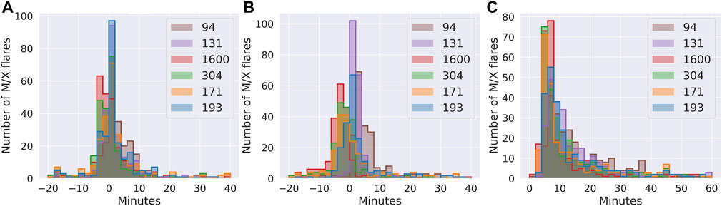
FIGURE 2. Comparison of start and peak times for flaring as measured in AIA. (A), discrepancy in minutes between AIA flare start times and GOES flare start times. (B), discrepancy in minutes between AIA flare peak times and GOES flare peak times (note that the GOES flare catalog does not contain peak times for flares after 2017/06/30 so we only include available data). (C), time between flare start and peak for AIA flares.
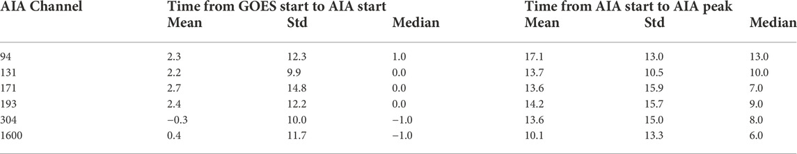
TABLE 2. Mean, standard deviation and median in minutes for comparison of flare timing in AIA channels vs. GOES.
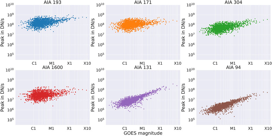
FIGURE 3. Peak intensity in AIA wavelengths as a function of GOES flare magnitude. Units of AIA intensity are “Data Numbers” (DN) per second, i.e., raw detector output not calibrated to irradiance units. In all cases, decreasing GOES magnitude is associated with higher spread in AIA intensities. The 131 and 94 Å channels show the tightest correlation with GOES X-ray magnitudes.
4 Estimating flare magnitudes with AIA data using ML-based regression
The results of the previous section show that we can identify flares of various magnitudes solely from the AIA SHARP summed-pixel time series. These identifications have the advantage over GOES flare identifications of being automatically associated with a particular SHARP active region, thus eliminating the potential for error in location assignment that characterizes the GOES process. We note that SHARP active region designations do not always match the official NOAA AR designations: there are cases where one SHARP region includes two or more NOAA AR designations. The mapping between SHARP numbers and NOAA AR numbers is available from the SDO Joint Science Operations Center (JSOC)5. In addition to defining the timing and location of flaring events based on AIA data, we show that we can also correlate these events to historical X-ray magnitudes using a machine-learning regression model, thus leading us to a full AIA-based flare catalog.
4.1 ML architecture and data input
Experiments were conducted using an extremely randomized trees (ERT) model with input features extracted from AIA images and SHARP meta-data. An ERT is a type of ensemble method, where the base estimators are decision trees and the final output is computed by averaging the results of all the individual estimators (Geurts et al., 2006). Ensemble methods are often used to reduce variance or bias that can result from a single estimator. ERTs and other tree-based ensemble methods such as random forests (Breiman, 2001), although relatively simple machine learning models, have been shown to be broadly applicable to both classification and regression problems [see (Boulesteix et al., 2012; Criminisi et al., 2012; Biau and Scornet, 2016) and references within]. Decision trees themselves are fundamental ML models that are often used to introduce the ideas of ML-based classification, as in (Murphy, 2022). Each decision tree is built starting with a base node and splitting the data based on a feature or set of features; this process continues iteratively until a maximum depth or minimum impurity is achieved. The splitting criteria at each node is chosen to minimize some loss metric – here we find the minimum absolute error (MAE) to perform the best. In an ERT, the full data set is used to construct each tree, many candidate splitting thresholds for each feature are randomly generated at each node, and the best split is chosen from these. We use the sklearn implementation in Python of an ERT regressor.
The ERT model operates on features obtained from AIA SHARPs and HMI SHARP metadata. All 6 AIA wavelengths are used. For each AIA wavelength (94, 131, 304, 171, 193, and 1600 Å), we consider the following features: the peak summed-pixel value over the flare in DN/s (λ_magnitude), the difference between that peak and the summed-pixel value at the flare start time in DN/s (λ_rel_magnitude), the maximum number of saturated pixels in the AIA cutout over the duration of the flare (λ_est_size), and the duration of the flare in seconds (λ_duration). Also included is the size of the AIA cutouts, Nx and Ny. The full set of input features is given in Table 3. The HMI SHARP parameters are available in the SDO/HMI dataset metadata and are a standard set of physics-based features chosen for their flare predictive abilities (Bobra et al., 2014). All input features are normalized to have zero mean and unit variance based on the training data. The output of the model is the GOES X-ray flare magnitude, normalized by taking the log and scaling between 0 and 1. The model is trained on the input features and corresponding output labels, and then can be used to estimate outputs based on new input data that were not included in the training set.
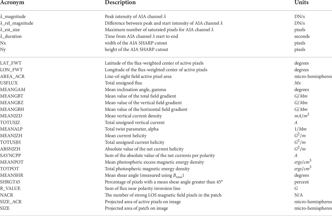
TABLE 3. AIA and HMI SHARP based features for the ERT model. For AIA based features with channel λ, we consider all 6 wavelengths
There are several hyperparameters that can be adjusted for ERT models. We perform hyperparameter tuning using 5-fold cross validation to determine the number of decision trees and the minimum impurity decrease, or Gini impurity index, which is a threshold for when to stop splitting the decision trees. The data is split into 80% training and 20% testing for 10 different random seeds. A 5-fold cross validation is performed on the training data of each of these 10 seeds and the final parameters are chosen based on the best results across experiments. The tuned model has 100 decision trees and a Gini impurity index of 4e-5.
4.2 Results
The data was split by flare category so that the same proportion of C, M and X flares were in the training and test set. Only flares found by the peak finding algorithm and by the manual verification process described in Section 3 that have an associated GOES flare were included in both the training and test data, in order to have a true flare magnitude label associated with the data.
To evaluate our results we consider four metrics: the root mean squared error (RMSE), the mean absolute error (MAE), the coefficient of determination or R2 score, and the relative L2 error. These are computed as follows,
where yi are the true values and
A comparison between the ERT results is shown in Table 4, where all metrics are evaluated in log of X-ray magnitude of the test data. We can see that only using physics based HMI SHARPs features is insufficient for determining flare magnitudes, but using AIA SHARPs based features we can estimate flare magnitudes with high accuracy. Given that the standard deviations for the metrics given in Table 4 are so low, we show results from a single seed, that is, closest to the mean result in Figure 4. Figure 4A shows the experiments with AIA SHARPs features only and Figure 4B shows both AIA and HMI SHARPs. We notice that: 1) adding HMI SHARPs features makes insignificant difference, and 2) there tends to be a slight under prediction for C-class flares.
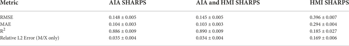
TABLE 4. Comparison of results for different input features where metrics are given in terms of the average over the 10 random seeds ± the standard deviation. These metrics are evaluated in log of X-ray magnitude.
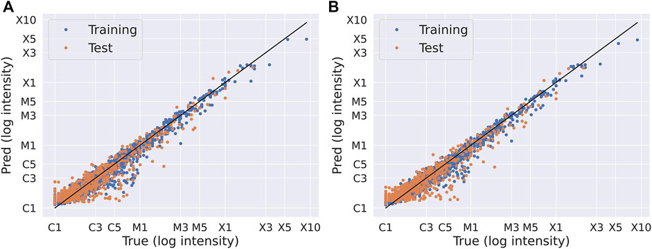
FIGURE 4. Predicted vs. true flare magnitudes using AIA SHARPS features for both training and test data, (A) AIA SHARPs features only, (B) AIA and HMI SHARPs features. The closest seed to the mean result in Table 4 is depicted, which is a different split for each feature set.
One advantage of ERT models is their interpretability. Figure 5 shows the feature ranking in terms of the Gini importance (a measure of how much each feature contributes to improving the decision tree splitting) for the top 20 inputs to the ERT models for the experiment with the full AIA and HMI SHARPs based features. Any additional features are not shown because they are essentially irrelevant for the ERT prediction. These included the vast majority of HMI SHARPs features. Of interesting note, the location of the cutout on the disk is irrelevant. This indicates that flaring is isotropic over the disk and that EUV scales with X-ray flare magnitude.
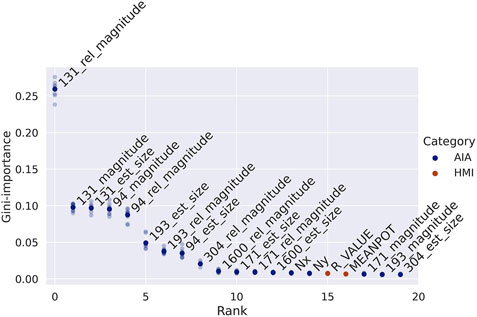
FIGURE 5. Feature importance rankings for the experiment with both AIA and HMI SHARPs features (right). The results from each random seed are shown in faint colors, while the dark colored dots depict the average importance. Only the top 20 features are shown.
4.3 Estimating magnitudes of flares without GOES labels
Using the trained model, we can estimate flare magnitudes for AIA peaks which are not associated with a GOES flare. The majority of these peaks are small, and thus not important for predicting large flares. However, we are able to find and manually verify an additional 62 M flares and 2 X flares based on the magnitudes estimated by the ERT, which do exhibit a peak in the raw GOES X-ray data, but do not appear in the GOES flare catalog. Most, but not all of these events appear in the HEK flare catalog (see link in Section 1).
5 Conclusion
Prior investigations have showed limited correlation between flare signatures in EUV and X-ray (Mahajan et al., 2010; Le et al., 2011; Verbeeck et al., 2019). However, there have also been efforts to automatically detect flares using extreme ultraviolet SDO/AIA data (Martens et al., 2012; Kraaikamp and Verbeeck, 2015). In this work, we move beyond just detecting flares in AIA to correlating AIA based features to the GOES X-ray flare magnitudes using a machine learning model, thus offering a way to define solar flares using AIA data and complement the GOES/XRS instrument as a tool for measuring flares. Using summed-intensity time series of AIA SHARPs cutouts in several wavelengths, we automatically detect peaks corresponding to flaring activity and denote start, peak and end times. We manually verify large M/X flares to corroborate our peak-finding results. Using features extracted from AIA images of flares, we then correlate to the corresponding X-ray flare magnitudes. An extremely randomized trees model trained on these features as well as physics-based features from the corresponding SHARP HMI image obtains 3.4% error in log magnitude on the test set for large M/X flares. However, it is noted that HMI SHARPs features are unnecessary. The result of this work is an AIA-based flare catalog, which we compare to the GOES X-ray flare catalog. Through this comparison we identify 20 mislabelled M/X flares in the GOES catalog and 64 M/X flares missing from the GOES catalog.
Given the popularity of supervised machine learning models for solar flare forecasting, it is critical that flare labels are accurate. Using an AIA-based flare catalog and incorporating AIA data as inputs, we hope to improve performance of solar flare forecasting machine learning models. Future areas of investigation include extending our extreme ultraviolet based catalog to SOHO/EIT data to add another decade of flare activity.
Data availability statement
The AIA data for this study was downloaded from JSOC at http://jsoc.stanford.edu/AIA/AIA_jsoc.html. The generated AIA catalog is available on Github at https://github.com/SWxTREC/aia-flare-catalog. A copy of the GOES catalog compared to in this study is also available within that repository.
Author contributions
KvdS designed the algorithms and models and performed the analysis under direction of NF and TB. RG conducted verification of the catalog. KvdS, NF, and TB discussed the results and contributed to the final manuscript.
Funding
This research was funded by NASA Space Weather O2R research grant 80NSSC20K1404 to the University of Colorado at Boulder, with GPU computational facilities provided by Air Force Office of Scientific Research DURIP grant FA9550-21-1-0267. TB was also supported by a Grand Challenge grant to the Space Weather Technology, Research, and Education Center at the University of Colorado at Boulder.
Acknowledgments
The authors would like to acknowledge Varad Deshmukh and Allison Liu for contributing to discussions during this work, as well as the members of the GOES data team at the NOAA National Center for Environmental Information (NCEI) and the CU Cooperative Institute for Research in Environmental Sciences (CIRES).
Conflict of interest
Author NF was employed by Flyer Research LLC.
The remaining authors declare that the research was conducted in the absence of any commercial or financial relationships that could be construed as a potential conflict of interest.
Publisher’s note
All claims expressed in this article are solely those of the authors and do not necessarily represent those of their affiliated organizations, or those of the publisher, the editors and the reviewers. Any product that may be evaluated in this article, or claim that may be made by its manufacturer, is not guaranteed or endorsed by the publisher.
Footnotes
1Historically the alphabetical scale stood for “Common”, “Medium”, and “eXtreme” flares. “A” and “B” flares were subsequently added below C flares to account for flares during solar minimum periods. See https://www.swpc.noaa.gov/products/goes-x-ray-flux for details on X-ray flare data and flare classification.
2Available at https://www.ngdc.noaa.gov/stp/space-weather/solar-data/solar-features/solar-flares/x-rays/goes/xrs/.
3Available at https://www.ngdc.noaa.gov/stp/satellite/goes-r.html.
4Available at https://www.lmsal.com/heksearch/.
5http://jsoc.stanford.edu/doc/data/hmi/harpnum_to_noaa/all_harps_with_noaa_ars.txt.
References
Barnes, G., Leka, K. D., Schrijver, C. J., Colak, T., Qahwaji, R., Ashamari, O. W., et al. (2016). A comparison of flare forecasting methods. I. results from the “All-Clear” workshop. Astrophys. J. 829, 89. doi:10.3847/0004-637X/829/2/89
Barnes, W. T., Cheung, M. C. M., Bobra, M. G., Boerner, P. F., Chintzoglou, G., Leonard, D., et al. (2020). aiapy: A Python package for analyzing solar EUV image data from AIA. J. Open Source Softw. 5, 2801. doi:10.21105/joss.02801
Biau, G., and Scornet, E. (2016). A random forest guided tour. Test 25, 197–227. doi:10.1007/s11749-016-0481-7
Bobra, M. G., and Couvidat, S. (2015). Solar flare prediction using SDO/HMI vector magnetic field data with a machine-learning algorithm. Astrophys. J. 798, 135. doi:10.1088/0004-637X/798/2/135
Bobra, M. G., Sun, X., Hoeksema, J. T., Turmon, M., Liu, Y., Hayashi, K., et al. (2014). The helioseismic and magnetic imager (HMI) vector magnetic field pipeline: SHARPs – space-weather HMI active region Patches. Sol. Phys. 289, 3549–3578. doi:10.1007/s11207-014-0529-3
Boulesteix, A. L., Janitza, S., Kruppa, J., and König, I. R. (2012). Overview of random forest methodology and practical guidance with emphasis on computational biology and bioinformatics. WIREs. Data Min. Knowl. Discov. 2, 493–507. doi:10.1002/widm.1072
Chamberlin, P. C., Woods, T. N., Eparvier, F. G., and Jones, A. R. (2009). Next generation X-ray sensor (XRS) for the NOAA GOES-R satellite series. Sol. Phys. Space Weather Instrum. III 7438, 743802. doi:10.1117/12.826807
Criminisi, A., Shotton, J., and Konukoglu, E. (2012). Decision forests: A unified framework for classification, regression, density estimation, manifold learning and semi-supervised learning. FNT. Comput. Graph. Vis. 7, 81–227. doi:10.1561/0600000035
Geurts, P., Ernst, D., and Wehenkel, L. (2006). Extremely randomized trees. Mach. Learn. 63, 3–42. doi:10.1007/s10994-006-6226-1
Jonas, E., Bobra, M., Shankar, V., Todd Hoeksema, J., and Recht, B. (2018). Flare prediction using photospheric and coronal image data. Sol. Phys. 293, 48. doi:10.1007/s11207-018-1258-9
Kraaikamp, E., and Verbeeck, C. (2015). Solar demon – An approach to detecting flares, dimmings, and EUV waves on SDO/AIA images. J. Space Weather Space Clim. 5, A18. doi:10.1051/swsc/2015019
Le, H., Liu, L., He, H., and Wan, W. (2011). Statistical analysis of solar EUV and X-ray flux enhancements induced by solar flares and its implication to upper atmosphere. J. Geophys. Res. 116. doi:10.1029/2011JA016704
Leka, K. D., Park, S. H., Kusano, K., Andries, J., Barnes, G., Bingham, S., et al. (2019a). A comparison of flare forecasting methods. III. systematic behaviors of operational solar flare forecasting systems. Astrophys. J. 881, 101. doi:10.3847/1538-4357/ab2e11
Leka, K. D., Park, S. H., Kusano, K., Andries, J., Barnes, G., Bingham, S., et al. (2019b). A comparison of flare forecasting methods. II. benchmarks, metrics, and performance results for operational solar flare forecasting systems. Astrophys. J. Suppl. Ser. 243, 36. doi:10.3847/1538-4365/ab2e12
Lemen, J. R., Title, A. M., Akin, D. J., Boerner, P. F., Chou, C., Drake, J. F., et al. (2012). The atmospheric imaging assembly (AIA) on the solar Dynamics observatory (SDO). Sol. Phys. 275, 17–40. doi:10.1007/s11207-011-9776-8
Mahajan, K. K., Lodhi, N. K., and Upadhayaya, A. K. (2010). Observations of X-ray and EUV fluxes during X-class solar flares and response of upper ionosphere. J. Geophys. Res. 115, n/a. doi:10.1029/2010JA015576
Martens, P. C. H., Attrill, G. D. R., Davey, A. R., Engell, A., Farid, S., Grigis, P. C., et al. (2012). Computer vision for the solar Dynamics observatory (SDO). Sol. Phys. 275, 79–113. doi:10.1007/s11207-010-9697-y
Murphy, K. P. (2022). Probabilistic machine learning: An introduction. Cambridge, Massachusetts: MIT press, 5–6.
Nishizuka, N., Sugiura, K., Kubo, Y., Den, M., Watari, S., and Ishii, M. (2017). Solar flare prediction model with three machine-learning algorithms using ultraviolet brightening and vector magnetograms. Astrophys. J. 835, 156. doi:10.3847/1538-4357/835/2/156
Park, S. H., Leka, K. D., Kusano, K., Andries, J., Barnes, G., Bingham, S., et al. (2020). A comparison of flare forecasting methods. IV. Evaluating consecutive-day forecasting patterns. Astrophys. J. 890, 124. doi:10.3847/1538-4357/ab65f0
Qahwaji, R., and Colak, T. (2007). Automatic short-term solar flare prediction using machine learning and sunspot associations. Sol. Phys. 241, 195–211. doi:10.1007/s11207-006-0272-5
Qian, L., Burns, A. G., Solomon, S. C., and Chamberlin, P. C. (2012). Solar flare impacts on ionospheric electrodyamics. Geophys. Res. Lett. 39. doi:10.1029/2012GL051102
Solomon, S. C. (2005). Solar extreme-ultraviolet irradiance for general circulation models. J. Geophys. Res. 110, A10306. doi:10.1029/2005JA011160
Tsurutani, B. T. (2005). The October 28, 2003 extreme EUV solar flare and resultant extreme ionospheric effects: Comparison to other Halloween events and the Bastille Day event. Geophys. Res. Lett. 32, L03S09. doi:10.1029/2004GL021475
Verbeeck, C., Kraaikamp, E., Ryan, D. F., and Podladchikova, O. (2019). Solar flare distributions: Lognormal instead of power law? Astrophys. J. 884, 50. doi:10.3847/1538-4357/ab3425
Keywords: solar flares, machine learning, catalogs, X-ray flares, EUV
Citation: van der Sande K, Flyer N, Berger TE and Gagnon R (2022) Solar flare catalog based on SDO/AIA EUV images: Composition and correlation with GOES/XRS X-ray flare magnitudes. Front. Astron. Space Sci. 9:1031211. doi: 10.3389/fspas.2022.1031211
Received: 29 August 2022; Accepted: 31 October 2022;
Published: 22 November 2022.
Edited by:
Yang Chen, University of Michigan, United StatesReviewed by:
Qiang Hu, University of Alabama in Huntsville, United StatesAlexey A. Kuznetsov, Institute of Solar-Terrestrial Physics (RAS), Russia
Copyright © 2022 van der Sande, Flyer, Berger and Gagnon. This is an open-access article distributed under the terms of the Creative Commons Attribution License (CC BY). The use, distribution or reproduction in other forums is permitted, provided the original author(s) and the copyright owner(s) are credited and that the original publication in this journal is cited, in accordance with accepted academic practice. No use, distribution or reproduction is permitted which does not comply with these terms.
*Correspondence: Kiera van der Sande, a2llcmEudmFuZGVyc2FuZGVAY29sb3JhZG8uZWR1