Abstract
Meteor observations provide information about Solar System constituents and their influx onto Earth, their interaction processes in the atmosphere, as well as the neutral dynamics of the upper atmosphere. This study presents optical, radar, and infrasound measurements of a daytime fireball that occurred on 4 December 2020 at 13:30 UTC over Northeast Sweden. The fireball was recorded with two video cameras, allowing a trajectory determination to be made. The orbital parameters are compatible with the Northern Taurid meteor shower. The dynamic mass estimate based on the optical trajectory was found to be 0.6–1.7 kg, but this estimate can greatly vary from the true entry mass significantly due to the assumptions made. The meteor trail plasma was observed with an ionosonde as a sporadic E-like ionogram trace that lasted for 30 min. Infrasound emissions were detected at two sites, having propagation times consistent with a source location at an altitude of 80–90 km. Two VHF specular meteor radars observed a 6 minute long non-specular range spread trail echo as well as a faint head echo. Combined interferometric range-Doppler analysis of the meteor trail echoes at the two radars, allowed estimation of the mesospheric horizontal wind altitude profile, as well as tracking of the gradual deformation of the trail over time due to a prevailing neutral wind shear. This combined analysis indicates that the radar measurements of long-lived non-specular range-spread meteor trails produced by larger meteoroids can be used to measure the meteor radiant by observing the line traveled by the meteor. Furthermore, a multistatic meteor radar observation of these types of events can be used to estimate mesospheric neutral wind altitude profiles.
Introduction
On 13:30:38 4 December 2020 (UTC), a 6.5 s long daylight fireball was observed in Northern Scandinavia. Eyewitness accounts of the bright fireball were reported in the local newspaper (Medby, 2020). The reports included observations of a greenish color and fragmentation. There were no observations of audible rumble nor were there any meteorite findings. Several photographs of the fireball are shown in Figure 2.
The event occurred in a geographic region that is relatively well instrumented for atmospheric studies allowing us to report on a wide variety of atmospheric effects associated with fireballs. The optical signature was captured by two video cameras of the Norwegian meteor network, which were used to estimate a trajectory across Northwest Finland and ending above the village of Pajala. Cameras in Sweden and Finland did not observe the fireball due to dense cloud cover. In the geographic region surrounding the trajectory of the fireball, five specular meteor radars and three ionosondes recorded the echoes from plasma density irregularities created by the meteor. Two infrasound monitoring stations measured pressure waves that could be associated with this event. An overview of the observations of this event is shown in Figure 1.
FIGURE 1

Summary of the observations of the fireball on 4 December 2020 at 13:30 UTC.
The primary focus of this study is to present and discuss the observations associated with the Pajala fireball. These multi-instrument measurements allow us to: 1) estimate the orbital elements and the entry mass of the meteoroid, 2) compare the plasma trail characteristics with existing theories of the governing physical processes associated with meteor trail plasma evolution, and 3) study mesospheric neutral wind with high spatial and temporal resolution.
Optical observations
The Sørreisa and Skibotn stations of the Norwegian meteor network observed the optical path of the fireball. Both stations have all-sky coverage obtained with four Vivotek IP9171 security cameras that have 2048 × 1536 RGB pixel CMOS sensors. The Sørreisa camera acquired 14 frames per second and the Skibotn camera 15 frames per second. The output was compressed with the H.264 video compression algorithm (Wiegand et al., 2003). The cameras are timed using network time protocol. The field of view of the camera across the diagonal of the sensor was approximately 115° for Skibotn and 136° for Sørreisa. Simultaneous frame captures from the Skibotn and Sørreisa cameras are shown on the left in Figure 2.
FIGURE 2

On the left, video camera stills of the fireball from two observing stations at 2020-12-04 13:30:42 UTC. The view from Skibotn is shown above (A) and the view from Sørreisa is shown below (B). On the right, there is an image (C) of the fireball taken by John M. Oskal in Sørreisa using a smartphone camera.
In order to estimate the trajectory of the meteoroid, a star calibration with approximately 100 stars covering the full camera field of view was performed using a technique described by Gustavsson et al. (2008). For the geometric camera calibration we found that a camera model:Was sufficient to accurately represent the mapping of light from a direction in space to the horizontal, u, and vertical, v, coordinates. Here θ is the polar angle from the optical axes of the camera, ϕ is the azimuthal angle; fu and fv are the horizontal and vertical focal widths; u0 and v0 are the horizontal and vertical image-coordinates of the optical axis, and κ is a shape-parameter. In addition three rotation-angles (ψi) are used to determine the rotation of the camera. This in total leads to 8 parameters (fu, fv, u0, v0, κ, ψ1, ψ2, ψ3) that determine the mapping of light from a direction (azimuth, zenith) to image-pixels (u, v).
To make it possible to identify a sensible number of stars, we integrate the intensity from 225 frames after background reduction with a 9-by-9 pixel median-filter. This made it straightforward to identify 78 stars from Skibotn, which is shown in Figure 3. The calibration sources selected from the bright star catalogue (Hoffleit and Warren Jr, 1987). The standard deviation of the differences between the centroids of the identified stars in the image and the corresponding points calculated with the calibrated camera-model are 0.39 pixels in the horizontal direction and 0.35 pixels in the vertical direction. The residuals for all calibration sources are shown in Figure 4. The calibration error coresponds to a pointing-uncertainty of 0.02° in the fire-ball part of the image. The procedure produced similar calibrations for the images from Sorreisa and Skibotn.
FIGURE 3

An example star calibration image during the first clear night after the fireball (2020-12-07T01:01:55Z).
FIGURE 4

Position residuals for calibration sources in the Skibotn camera in units of pixels in the horizontal and vertical direction.
The centroid position of the fireball was manually determined from each frame of the video recording. The trajectory was then determined by searching for the shortest line of sight intersection using a technique similar to the one described by Vida et al. (2020). Linear interpolation of inter-frame pixel position was used to align the timings of the frames obtained with the two stations. The RMS uncertainty in Earth Centered Earth Fixed (ECEF) coordinates for the estimated trajectory was estimated to be 384, 1,060, and 214 m in the x, y, and z directions based on the fit residuals.
Within the brightest portion of the trajectory, the intensity of the fireball was saturated, making it difficult to obtain a good estimate for brightness. A rough estimate for apparent brightness magnitude of −13 is based on the similarity of the brightness of the fireball to the brightness of the full Moon in similar lighting conditions and camera settings.
Orbital parameters
In order to estimate the velocity vector v (0) at atmospheric entry, a model with an exponentially increasing atmospheric drag (Whipple and Jacchia, 1957; Jansen-Sturgeon et al., 2020) was fit using the least-squares method to the measured optical positions as a function of time:Here and are parameters describing the atmospheric drag, is the magnitude of the entry velocity, and is a unit vector describing the initial velocity vector direction, and x0 is the initial position. The distribution of the estimated parameters x0, , v0, a0 and a1 were sampled using the Single Component Adaptive Metropolis-Hastings (MCMC) algorithm (Haario et al., 2005).
In order to remove the effect of Earth’s gravity on the orbital parameters, the REBOUND N-body code (Rein and Liu, 2012) was used to propagate the position of the object back in time by 16 h, to a position before the object entered the sphere of influence of Earth’s gravity. The simulations were integrated using IAS15, a 15th order Gauss-Radau integrator (Rein and Spiegel, 2015). The uncertainty of orbital parameters was obtained using the MCMC samples obtained when fitting Eqs 3, 4. The estimated orbital parameters in the Heliocentric Mean Ecliptic J2000 frame are shown in Table 1. The propagation included perturbations from all planets and the Moon, and initial states of these bodies at the epoch of observation were generated using the JPL DE430 planetary ephemerides (Folkner et al., 2014). The table also shows the estimated Cartesian state in the J2000 instance of the International Terrestrial Reference Frame (ITRF) (Altamimi et al., 2002), as well as the apparent radiant without any corrections for the effects of Earth’s gravity.
TABLE 1
| Orbital parameters | |
|---|---|
| a | 2.26 ± 0.02 (AU) |
| e | 0.797 ± 0.002 |
| i | 3.21 ± 0.03 (deg) |
| ω | 281.76 ± 0.21 (deg) |
| Ω | 252.57651 ± 10–5 (deg) |
| ν | 257.7 ± 0.21 (deg) |
| Epoch | 2020-12-03 21:16:37 (UTC) |
| Tisserand parameter | 3.1 ± 0.02 (Jupiter) |
| Entry parameters | |
| x, y, z | 2,135.73, 1,007.27, 6,014.56 ± 0.05, 0.15, 0.06 km (ITRF) |
| v x , vy, vz | 22.72, −8.26, −14.00 ± 0.04, 0.06, 0.02 km s−1 (ITRF) |
| v 0 | 27.94 ± 0.09 km s−1 |
| RA | 76.06 ± 0.12 (deg) |
| Dec | 30.03 ± 0.01 (deg) |
| λ ⊙ | 252.01 (deg) |
| Time of entry | 2020-12-04T13:30:37.5Z (UTC) |
Orbital parameters. Note that the orbital parameters with zenithal attraction removed are using an epoch 16.23 h before atmospheric entry. The radiant is reported as the apparent radiant, without removal of Earth’s gravitational effect.
To determine a origin of the meteoroid, long term backwards propagation of the entire probability distribution of possible orbits is needed. Such a propagation should be limited by chaos indicators and may hence not yield an association (e.g., Cincotta and Simó, 2000). Additionally, during this backwards propagation, there are several metrics that can be used to indicate dynamical association (Trigo-Rodriguez et al., 2007; Peña-Asensio et al., 2022). However, such an in depth dynamical investigation is outside the scope of the current study.
Instead, a first order examination of the origin of the object can be made using three methods: 1) orbital similarity criteria at time of detection, 2) cometary versus asteroidal classification criteria, and 3) comparison with known meteor showers.
Applying the two recommended cometary origin criteria proposed in Jopek and Williams (2013), the “Q-i” criterion (Q < 4.6 AU or i > 75°) failed with a Q = 4.06 AU and i = 3.2°, as well as the “E-i” criterion ( D−2 or i > 75°) with a D−2. As such both criteria indicate asteroidal origin. As is also noted in Jopek and Williams (2013), the asteroidal and cometary populations are not completely disjointed.
The observed object is compatible with the Northern Taurids meteor shower. When taking into account radiant drift and radiant distribution width derived from a catalogue of optical observations (Jenniskens et al., 2016), the Northern Taurids would have a radiant of α = 81.9° ± 5.2° and δ = 29.0° ± 1.6° with one standard deviation radiant width at the time of the fireball detection. The radiant derived from meteor radar observations (Brown et al., 2010) would predict a radiant position of α = 80.3° and δ = 25° at the time of the fireball detection. These are compatible with the values we derived for the Pajala fireball in Table 1, although the right ascension is slightly outside of one standard deviation. The velocity at atmospheric entry derived for the fireball also fits with the previously reported 28.0 km/s (Jenniskens et al., 2016). Therefore it is plausible that the object is associated with the Comet Encke complex.
Using the Near-Earth Asteroid and Comet databases available at the JPL Small-Body Database Search Engine 1 we applied the Southworth and Hawkins (1963)DSH function to search for similar objects. The best match to the Comet database also gave 2P/Encke, but with C/2002 R5 (SOHO) also returning a similar DSH value.
As the object could not be clearly defined as cometary or asteroidal, we also performed a DSH search trough the Near-Earth asteroid database. The Apollo asteroid 2008 XM1 as a very close best match together with many other Apollo asteroids. If one would restrict the search to only asteroids with an available size estimate above 1 km in diameter, the best match was 5,143 Heracles (1991 VL).
Dynamic mass
In order to estimate the mass from the velocity and acceleration of the object, the method introduced by Ceplecha (1966) was used. The derivation is discussed by several authors (see Gritsevich (2008) or Jansen-Sturgeon et al. (2020) and references therein). The atmospheric drag force for a high velocity object is assumed to be described by:with md the mass of the object, the deceleration, cd the drag coefficient, ρa the atmospheric density, v the velocity, and S the cross-sectional area of the object. The shape of the object is assumed to be brick-like with side lengths 2L, 3L, and 5L as described by Halliday et al. (1996), with L a scaling constant defining the size of the object. This leads to md = 30ρmL3 and S = 15L2. Here ρm is the density of the meteoroid. Assuming that cd = 1, the dynamic mass md can be estimated from Eq. 5 as:The acceleration and velocity are determined from the exponential velocity fit given in Eq. 3, with uncertainty propagated using the same MCMC samples. The atmospheric density ρa was determined using the MSIS model (Hedin, 1991).
The left panel of Figure 5 shows the estimated velocity as a function of altitude. The right panel of the same figure shows the estimated dynamic mass using three different object densities: 4 g/cm3, 1.7 g/cm3, and 0.6 g/cm3.
FIGURE 5
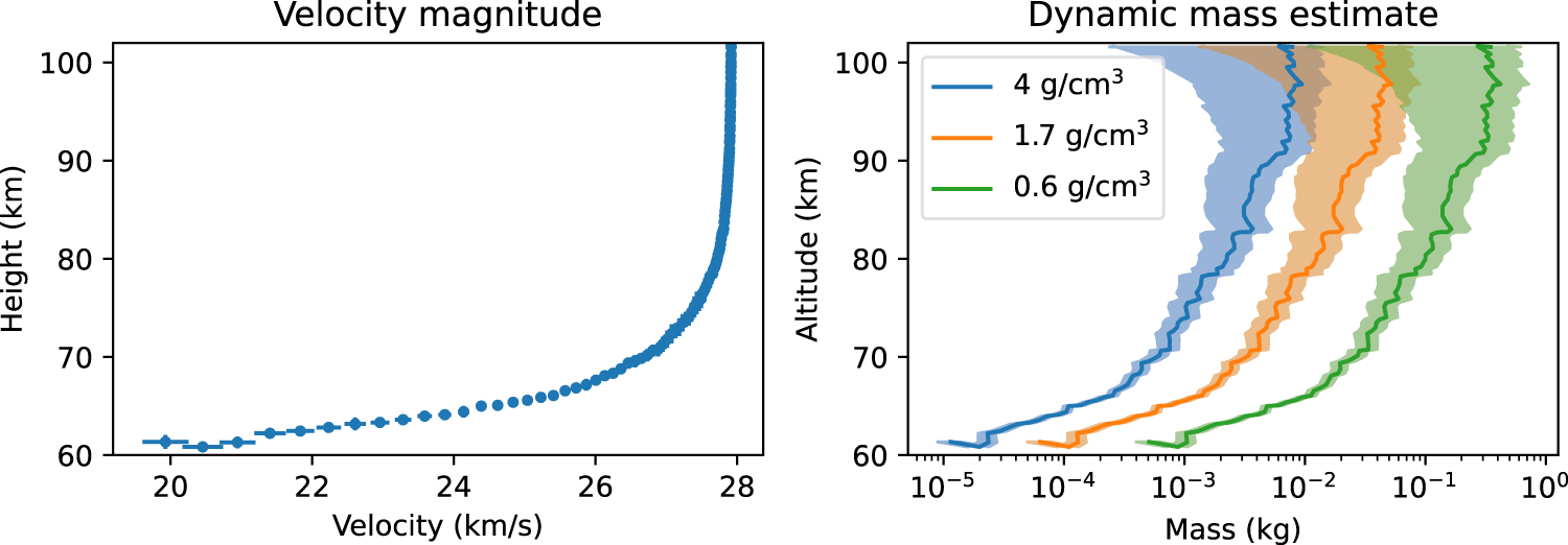
Left: The absolute magnitude of the measured velocity as a function of altitude. Two standard deviation errors in velocity and height are indicated. Right: Three different dynamic masses estimated from the meteor trajectory. The error estimates are two standard deviations.
An analysis of the ballistic coefficient and mass loss (Gritsevich, 2009) was performed using an implementation provided by Sansom et al. (2019). The derived ballistic coefficient is quite large (α = 680), as is the mass loss parameter (β = 4.2). They are both on the high end of the distribution compared to what is usually reported in the literature (Gritsevich, 2009; Sansom et al., 2019; Moreno-Ibáñez et al., 2020; Peña-Asensio et al., 2021; Boaca et al., 2022). The value of β indicates intensive mass loss, and a fairly large ballistic coefficient is due to the small initial mass. The effect is enhanced also by shallow entry angle of γ = 14.1° with respect to local horizon. This suggests that the meteor material is fairly fragile and volatile, implying a low-density meteoritic material. Due to the observed high mass loss rate, no meteorites are expected to make it down to the ground (Gritsevich et al., 2012; Sansom et al., 2019; Boaca et al., 2022).
The dynamic mass estimate is highly dependent on the density of the meteoroid, due to the term. The determined orbit is compatible with the Comet Encke complex, and the α − β analysis also indicates a low density material. If we assume cometary meteoroid density of 0.6 g/cm3, we find a dynamic mass of 323 ± 120 g. Figure 5 also shows the dynamic masses estimated for densities of 4 and 1.7 g/cm3, which yield much lower masses. The dynamic mass estimate is typically considered to be an underestimate of the object mass, especially if fragmentation occurred. Typically the dynamic mass is multiplied by a factor of 3-4 to take into account underestimation of entry mass due to fragmentation (Gritsevich, 2008). And in this case, there were several reports of fragmentantation and the optical observations showed at least two separate fragments at the end of the trajectory at 60 km altitude. Assuming a cometary density of 0.6 g/cm3 and applying a multiplicative factor of 3-4 would provide a mass estimate in the range 0.6–1.7 kg. However, there is considerable uncertainty related to shape, object density, fragmentation, and atmospheric density, which can increase or decrease the size estimate easily by an order of magnitude.
Meteor radar observations
There are five interferometric specular meteor radars (SMRs) operating in the geographic region surrounding the fireball trajectory. The primary use of these radars is to measure the mesosphere and lower thermospheric wind and temperature from observing specular meteor trail echoes (Hocking et al., 2001; Holdsworth et al., 2004). However, only three of these systems (Andenes, Tromsø, and Sodankylä) where configured to record raw voltage data. The routine analysis procedure discards any echoes that are not considered to be short duration specular meteor trail echoes, and therefore the systems that did not store raw voltage only retained a handful of detections associated with this event, which were falsely detected as specular meteor trail echoes. Most of the range extent of the radar echo associated with the fireball could be observed in the Sodankylä and Andenes radars, on the other hand, a large fraction of the trail echo in the Tromsø system overlapped with the transmit window.
In this study, we will focus on the Sodankylä and Andenes radar measurements. Both of the radar systems observed a long-lived range-spread radar echo as well as portions of the head echo.
Head echo
Both the Andenes and Sodankylä radars observed a head-echo return, which is due to scattering from the plasma surrounding the ablating meteoroid (see Figure 6). The expected one-way range based on optical observations is overlaid in Figure 6, which matches relatively well with the location of the head echo. These types of echoes are routinely observed with eight orders of magnitude more sensitive high power large aperture radars, which can observe head echoes associated with meteoroids in the mass range between 10–9 − 10–3 g (Flynn, 2002). For a review, refer to Kero et al. (2019) and references therein. On rare occasions, head echoes can be observed with SMRs (Schult et al., 2015; Marshall et al., 2017; Chau et al., 2021), but they are associated with large fireballs and bolide-class events.
FIGURE 6

The head echo observed with the Sodankylä and Andenes meteor radars.
Neither the Sodankylä nor the Andenes radar is calibrated for accurate power measurements. However, a rough estimate of the radar cross-section of the head echo can be made. This estimation is complicated by the fact that the Sodankylä radar used a four-pulse coherent integration, which attenuates some of the head echoes at some ranges. We have attempted to remove the effect of coherent integration on the signal-to-noise ratio (SNR) using the inverse magnitude response of an analytic four-sample averaging filter. The Andenes system did not use this type of a coherent integration filter, but in this case, the RCS estimation was complicated by the relatively low elevation angle (≈10°), which increases the uncertainty associated with antenna gain. We have used the antenna gain pattern given by Singer et al. (2004) in our calculations.
The estimated radar cross-section for the Sodankylä and Andenes radars is shown in Figure 7. The regions of the range-time-intensity measurement that are used to estimate RCS, i.e. σ, are indicated with a light blue color in Figure 6. The Sodankylä radar has a gap in detectable head echo between 185 and 195 km. This can be due to the four-pulse coherent integration filter. It is also possible that differential ablation from Na and K (Vondrak et al., 2008) can contribute to the presence of this gap.
FIGURE 7

Estimates of the radar cross-section as a function of altitude. The normalized magnitude response of the four-pulse coherent integration window of the Sodankylä radar is also included, with Doppler frequency based on the estimated trajectory. The estimates for Sodankylä are corrected for the frequency response of the coherent integration used by the radar.
Both the Andenes and Sodankylä radars produce compatible estimates of the radar-cross-section, peaking at approximately σ = 1.7 ⋅ 104 m2 or 42 dBsm at 92 km altitude. This radar cross-section is comparable with the largest reported radar cross-section observed with CMOR over a 10 month period by Marshall et al. (2017).
As seen in Figure 6, at t = 35–40 s, the head echo is slightly delayed from the range predicted by the trajectory. A possible explanation for this is intense fragmentation of the object. In this case, fragments that have been detached from the main body continue to ablate and produce a dense plasma, but trail the main body.
It is unlikely that a good ionization mass estimate from the radar observations can be made for the fireball, as the head echo could not be observed at altitudes below 90 km where much of the mass loss occurred based on the optical trajectory. Also, the literature that discusses models for ionization probability and ionization line density specifically state that the models are only valid for much smaller meteors (e.g., Jones, 1997; Marshall et al., 2017).
Long-duration trail echo
The radar echoes for the long-lived trail echo were processed using a range-Doppler analysis procedure similar to that used in MST radars. The echoes were first analyzed using a windowed pulse-to-pulse fast Fourier transform for each range. Several windows over a 10 s time period were then averaged together to form an estimate of the scattered radar signals as a function of range and Doppler.
The range-spread trail echo observed with the Sodankylä and Andenes radars is shown in Figure 8. The left hand side shows the SNR as a function of time and one-way range. The right hand side shows the estimated peak Doppler shift of the echo. The trail duration is approximately 370 s on both radars. Only a small portion of the trail echo observed in Sodankylä had a specular geometry, based on the estimated optical trajectory. The scattering geometry also made it impossible for any portion of the trail to have the Bragg scattering wave vector perpendicular to the local geomagnetic field for either of the radars. Towards the end of the echo, the trail can be seen splitting into three discernible parts, due to action by the neutral wind.
FIGURE 8

The long-lasting range-spread trail echo observed in (A) Sodankylä and (B) Andenes. Signal-to-noise ratio is shown on the left and Doppler shift is shown on the right. Towards the end of the trail, the trail can be seen splitting into three discernible parts as the trail is being transported due to the mesospheric neutral wind.
Such range-spread echoes that do not have specular or perpendicular to magnetic field geometry have been previously reported by a few authors (e.g.,
Kelley et al., 1998;
Chau et al., 2014;
Kozlovsky et al., 2018,
2020) during observations of larger meteors. On the other hand, long-duration range-spread echoes observed perpendicular to the magnetic field have been observed by many authors (e.g.,
Kero et al., 2019, and references therein). Several physical mechanisms have been proposed to explain long-duration range-spread echoes in general. Here is a list of those that could be applicable to our observations, i.e., that do not require to point perpendicular to the magnetic field:
1) The presence of meteoric aerosols produced by the ablating meteor can increase the Schmidt number of the ion species. This increased Schmidt number in the presence of turbulence, would enhance the radar backscatter cross-section (Kelley et al., 1998; Chau et al., 2014). The needed turbulence could be due to the Kelvin-Helmholtz instability if the horizontal wind shear of the background atmosphere is large enough (Bernhardt, 2002).
2) Metallic ion chemistry (Baggaley, 1978; Maruyama et al., 2003; Plane, 2003) may deplete the controlling O3 species within the ambient atmosphere, slowing down the recombination.
3) The presence of a zonal wind shear can transport the plasma into a narrow layer (Whitehead, 1961; Mathews, 1998; Maruyama et al., 2003; Haldoupis, 2011).
We will attempt to investigate the role of the zonal wind shear later, but investigation of the other processes is beyond the scope of this study, as this would require a larger modeling effort, or measurements that are not obtainable for this event.
Trail echo location via interferometry
The Sodankylä radar was significantly closer to the meteoroid trajectory than Andenes, allowing a relatively high elevation (27–32°) observation of the trail echoes. The Sodankylä radar also has seven interferometric receiver antennas, which improves the angle of arrival estimate quality compared to the standard five antennas. Due to these two reasons, we were able to conduct interferometric angle of arrival estimation for the radar echoes with relatively good accuracy.
In order to estimate the positions of the trail echoes, we calculated cross-spectra for each of the 21 unique antenna pairs. Each cross-spectrum was calculated over 0.5 s of time using a pulse-to-pulse discrete Fourier transform that to which a Hann tapering window function was applied to. Cross-spectra were incoherently averaged over 10 s to obtain a set of cross-correlations as a function of range and Doppler shift.
The interferometric angle of arrival of each range-Doppler bin was made separately using a single scattering source location model:Here r and ω are the range and Doppler shift of the scattered electromagnetic wave, Pab(r, ω) is scattered signal power, k (r, ω) is the wave vector of the scattered signal plane wave observed by the interferometer, za (r, ω) and za (r, ω) are the complex baseband signals observed on antennas a and b, and pa and pb are the positions of antennas a and b.
The azimuth and elevation for the angle of arrival was determined using a matched filter:In practice, this equates to digital beamforming of the seven antennas to dense grid of angles of arrival and choosing the direction that maximizes signal power observed across the interferometer (Chau and Clahsen, 2019). Each range and Doppler shift is allowed to have an independent angle of arrival, which is estimated separately.
The estimated positions of the scattering from the trail are shown in Figures 9A–D for four 10-s time intervals at 0–10, 50–60, 150–160, and 290–300 s after meteoroid entry. During the first 10 s after atmospheric entry of the meteoroid, the trail position is a line that tracks the path of the fireball, as expected. When comparing Figure 9A with Figure 1, the positions of the trail echoes are nearly identical to the positions of the fireball estimated from the dual video camera measurements. The difference in position of the radar trail and the optical trajectory is less than 10 km. This is presumably due to errors in estimating the position of the trail with radar. As time progresses, the trail is contracted in extent as diffusion and recombination acts on the trail faster on high and low altitudes. Echoes near the height of 92 km persist the longest.
FIGURE 9

Trail echo range-Doppler bin positions as a function of time. The amount of time after trail formation in each plot is (A) 0 − 10 s, (B) 50 − 60 s, (C) 150 − 160 s, (D) 290 − 300 s. The trail can be seen contracting due to ambipolar diffusion and recombination. The longest duration echo is observed at approximately 92 km altitude. The action of the neutral wind in the mesosphere can also be seen in the position of the trail echo, as a wind shear rotates and twists the trail. An animated sequence of radar images is provided as a supplement to this paper.
The action of the lower thermospheric neutral wind can be observed in the time evolution of the trail position, rotating and twisting the trail. Above 92 km, the trail can be seen migrating westward and below 92 km, the trail can be observed migrating eastward. This behaviour of trail deformation is similar to observations of chemiluminescent trail afterglows observed occasionally for larger meteors (Baggaley, 1975; Kelley et al., 2000), observations of rocket-based chemical release experiments that are used to trace neutral dynamics (e.g., Larsen, 2002, and references therein), or interferometric measurements of field aligned irregularities within meteor trails (Oppenheim et al., 2009). One primary difference between these types of trail measurements and chemical release experiments is that each measurement is also associated with a position and a radial Doppler shift, which tracks the neutral wind relatively quickly after trail formation.
The fact that the initial trail location as shown in Figure 9A is nearly identical to the trajectory estimated using cameras, indicates that these types of interferometric measurements of range-spread meteor trails can also be used to estimate the radiant of the meteor. We estimated the radiant of the meteor using the positions of the trail estimated using radar interferometry for the first 10 s after trail formation. The radar-echo based radiant was estimated to be at a right ascension of 76.53 ± 0.12° and a declination of 29.50 ± 0.10°, with errors estimated from the residuals of a fit of a line to the trail position. The radiant estimated from the meteor trail differs only by approximately 0.5° from the radiant estimated using cameras. There are two possible reasons for these deviations. 1) The interferometry was done over measurements of the trail position over the first 10 s. During this time, the trail is drifting with the background wind, which is shown in Figure 10. This drift will cause the trail orientation to change. 2) The azimuth and elevation dependent radar interferometer calibration errors may cause unmodeled position errors.
FIGURE 10

Estimated zonal and meridional wind velocity as a function of height, which is derived by combining the Sodankylä and Andenes meteor radar measurements of line of sight velocity.
Horizontal neutral wind
By using the Doppler shift estimated from the long lived trail with the Andenes and Sodankylä systems, it is possible to estimate a horizontal wind altitude profile. In order to make this estimate, we assume that the neutral wind only has a zonal and meridional component and that the Doppler shift of the meteor trail echo reflects the neutral wind.
In order to estimate the horizontal wind from the trail echo, we relied on the estimated trajectory, which was based on the interferometric positions of the echoes determined using the Sodankylä radar. We then used the observed trail echo Doppler shift observed with Andenes and Sodankylä as a function of altitude to estimate the horizontal wind using the following relationship:Here ωd is the observed Doppler shift, k is the Bragg scattering wave vector, vh is the horizontal wind vector, and ξ is the measurement error associated with Doppler shift. We express k and vh = [vm, vz, 0] in the local North-East-Down coordinate system at the position of the trail at each altitude, assuming that the vertical velocity is zero. Here vm and vz are the meridional and zonal components of the neutral wind.
Because we have two independent observations of Doppler shift with two linearly independent Bragg wave vectors, we can treat this as a linear regression problem of two independent measurements of Doppler shift and two unknowns vh, vz. This procedure is similar to the standard procedure for estimating mean horizontal wind using meteor radars, which is described by, e.g., Elford (1959).
In the case of the Sodankylä system, there is not a one-to-one mapping between range and height. In order to map trail Doppler shift to geographic position, we used the interferometric direction of arrival to map observed range and Doppler shift to height along the path of the trajectory. With the Andenes system there is a one-to-one mapping between one-way range and altitude, since the meteor is approaching the radar for the whole time. In this case, we can simply map the estimated trail Doppler shift as a function of range to height along the observed trail trajectory that is determined using the Sodankylä system.
The estimated horizontal wind velocity as a function of height is shown in Figure 10. The horizontal wind is also depicted on a map in Figure 11, where the positions of the arrows indicate the location where the wind is measured, the color indicates the altitude, and the direction and length of the arrows indicate the horizontal wind direction and magnitude. The estimated horizontal wind was compared with the regionally averaged, 1-h wind profile derived from specular meteor radars in the surrounding region. While this profile was not exactly the same, a similar general direction was observed. One key difference between the averaged wind estimate and the estimate shown in Figure 10 is the larger vertical gradient and shorter vertical wavelength. This is presumably due to the fact that the wind estimated from the fireball covers a smaller geographic region and a significantly shorter period of time (20 s vs 1 hour). While it cannot be conclusively proven that the wind estimated from the fireball trail is unbiased and accurate, it is expected that on small horizontal spatial and short temporal scales, there are significant fluctuations due to gravity waves that are not correlated over larger scales (e.g., Larsen, 2002; Vierinen et al., 2019).
FIGURE 11

The horizontal wind estimated from the long-lasting trail echo, overlaid on the locations of the trail map. The color indicates the trail echo height, and the white arrows indicate the magnitude and direction of the horizontal wind velocity estimated from the trail echo Doppler shifts observed with the Andenes and Sodankylä radars. Note that the deformation of the meteor trail shown in Figure 9 is in agreement with these velocities.
In order to study the role of Kelvin-Helmholtz instability (KHI) on creating turbulence that can contribute to the long duration trail echo, we can study the Richardson numberA sufficient condition for growth of the Kelvin-Helmholtz instability (KHI) is that Ri < 0.25. We can estimate this quantity from the horizontal velocity profile shown in Figure 10. We again need to make the assumption that the horizontal velocity estimated along the trajectory is a measurement of the prevailing horizontal velocity profile within a region of approximately 100 km horizontal extent. Assuming a 4-min Brunt-Väisälä period corresponding to an angular frequency of N = 2π ⋅ (4 ⋅ 60)−1 rad s−1, we get a Richardson number that at its minimum is Ri = 0.35 [0.15, 2.2] at 93 km. However, the uncertainty in the estimate is extremely large, making it impossible to draw definitive conclusions about the presence of KHI.
While meteor radars are already used for measuring the horizontal component of the lower thermospheric wind, this is primarily done using specular meteor trail echoes (e.g., Manning et al., 1950; Elford, 2001), which provide a nearly point like measurement in space, unlike the profile we observed. It is also known that field aligned plasma irregularities within meteoric plasma trails (Oppenheim et al., 2009, 2014), and plasma turbulence created within the wakes of larger meteors (Kelley et al., 1998; Chau et al., 2014) can also be used to measure the mesospheric neutral wind. However, these techniques have so far not gained wide-spread adoption, even though they could potentially be used as tracers of mesospheric wind, much like rocket experiments that use chemical (Larsen, 2002) or chaff releases (Koizumi et al., 2004). Especially during a meteor shower with an increased flux of larger meteors, this could be advantageous, as every range-spread meteor trail can potentially yield an independent profile of the mesospheric wind along the path of the meteor as shown in Figure 11. Long-lived range-spread meteor trails, as the one observed during this fireball, are relatively frequently observable during meteor shower times (Kozlovsky et al., 2020).
Ionosonde observations
The Sodankylä ionosonde “Alpha Wolf” is a frequency-modulated continuous-wave chirp sounder developed at Sodankylä Geophysical Observatory (SGO). Details of the instrument have been described by Enell et al. (2016). The ionosonde transmitter has a 64-m high rhombic antenna, and the receiver uses 20 orthogonal loop antennas located some 900 m from the transmitter. A sounding is made once a minute and each sweep lasts for 31 s, during which the transmitter frequency is linearly increased from 0.5 to 16 MHz. Although the ionosonde sounding is made once a minute, the time of transmission at a certain frequency is determined with much better accuracy. Indeed, the ionosonde starts transmitting 5 s before every integer minute and the transmitter frequency increases at a rate of 0.5 MHz/s. Typically, the uncertainty of the maximum frequency or the meteor echo obtained from ionograms is of the order of 0.5 MHz, so that the time accuracy is about 1 s.
The ionosonde started to observe enhanced ionization at 13:31:07 UT, 29 s after the meteor entry. It was seen as a sporadic layer (Es) reflecting radio waves at frequencies up to the highest one, i.e., foEs 16 MHz at a range of 165 ± 3 km (Figure 12). At the same range the Sodankylä meteor radar detected the meteor trail at an elevation 28.9° and azimuth 312.6° from N to E, which gives a height of 81.4 ± 1.5 km. This corresponds to an aspect angle close to 90° (Figure 13), such that the ionosonde backscatter is nearly specular. In the case of specular reflection from a cylindrical trail expanding due to ambipolar diffusion, the duration of the radio echo from an overdense trail at frequency f (i.e., foEs) is given bywhere αℓ is the electron line density of the trail, re = 2.82 ⋅ 10–15 m is the classical electron radius, c is the speed of light, and D is a diffusion coefficient (e.g., Maruyama et al., 2003). In such a case,with an exponent γ = 0.5. The maximal reflected frequency, foEs, was larger than 16 MHz during 5 min, until 13:36:20 UTC when it had decreased down to foEs = 13.0 MHz. Then the Es with decreasing foEs was observed until 13:40 UTC, after that the power of the echo got below the noise level. The time after meteor entry and corresponding maximal frequencies are given in Table 2.
FIGURE 12

Mono-static ionogram measured at 13:31 UTC using the Sodankylä Geophysical Observatory “Alpha Wolf” ionosonde.
FIGURE 13

Left: Aspect angle of the Sodankylä ionosonde radar scatter along the meteor trail determined using the trajectory triangulated with meteor cameras. The position indicated with a red cross is where the scattering is specular. The horizontal axis shows the one-way virtual height as seen in the ionogram in Figure 12. Right: The same, but for the oblique path between Sodankylä and Skibotn. In this case, the range on the horizontal axis is total propagation distance, assuming speed of light in vacuum, as shown in Figure 14.
TABLE 2
| Time (UTC) | Time (s) | foEs (MHz) | α ℓ (10–16 m−1) |
|---|---|---|---|
| 13:36:20.0 | 342 | 13.0 | 3.07 |
| 13:37:19.8 | 402 | 12.9 | 3.53 |
| 13:38:18.3 | 460 | 12.1 | 3.59 |
| 13:39:17.0 | 519 | 11.5 | 3.62 |
| 13:40:16.4 | 578 | 11.2 | 3.83 |
Plasma-frequencies and line densities as a function of time after the meteor entry.
According to the data presented in Table 2, the exponent γ = 0.32 ± 0.05, which means that in addition to the ambipolar diffusion another mechanism was responsible for evolution of the trail.
The right column in Table 2 shows the line electron density calculated from Eq. (11) using the diffusion coefficient obtained from the meteor radar data of the decay time of underdense meteor trails during 13:30 ± 3 h (it was D ≈ 3.4 m2/s near the 81.4 km height). This value, of the order of 3 ⋅ 1016 el./m, gives an upper limit estimate, because the trail was decaying slower than that given by Eq. (11).
The Sodankylä ionosonde transmissions were also received with an oblique path in Skibotn. This path saw a similar echo as the Sodankylä receiver, but the echoes related with the fireball were longer lasting, with a clearly discernible increased E-region plasma-frequency up to 1800 s after the atmospheric entry. Figure 14 (left) shows an example oblique ionogram with an E-region trace at 440 km virtual propagation distance, corresponding to the total propagation distance from Sodankylä to Skibotn, assuming a linear speed of light in vacuum propagation.
FIGURE 14

Left: The sporadic E trace that appeared after the fireball entry in the Sodankylä-Skibotn oblique ionogram. The horizontal trace at a virtual range of 440 km corresponds to the echoes from the meteor trail. The trace above 500 km is due to F-region O- and X-mode reflections. Right: maximum signal-to-noise ratio between 420-460 km as a function of time and frequency. The red line indicates the entry time of the fireball. The blue dots indicate points used to measure the decay rate of the cutoff frequency.
Figure 14 (right) also shows the SNR of the E-region trace as a function of time and frequency, with time measured in seconds since atmospheric entry. The peak frequency reflected by the trail is above 16 MHz for 850 s. It also takes several minutes before echoes at lower frequencies appear.
In the case of the Sodankylä-Skibotn path, the 80 km height also has a nearly perpendicular angle between the Bragg-scattering wave vector and the trail, and hence Eq. (12) should, to first order, be valid again. Using the blue dots in Figure 14, we obtain γ = 1.39 ± 0.08. This means that the trail was diffusing faster than expected, which is vastly different than in the mono-static case where the trail diffused more slowly than the theory predicts. One major difference here is that the oblique path is fit using time delays between 850 and 1900 s, whereas the mono-static case is fit with times delays between 342 and 578 s. The scales are also different.
Maruyama et al. (2003) suggested that the lifetime of the trails observed by ionosondes may be longer because of the wind shear deformation that causes a vertical divergence of electrons to a narrow layer. Using formulae 29.3 from (Haldoupis, 2011), we obtained vertical velocities 0.02 m/s and 3 ⋅ 10–5 m/s for 50 m/s zonal and meridional winds, respectively (the magnetic field inclination is 77.5°, ion-neutral collision frequency 105 s−1 at 81 km, and the ion gyrofrequency is 160 rad/s). Thus, this is not effective in the given case (near 81 km height).
Other factors affecting evolution of meteor trails are: recombination and attachment, which are important below 85 km to enhance the rate of de-ionization of Meteor smoke (dust) particles which slows down diffusion (e.g., Kelley et al., 1998; Shalimov and Kozlovskii, 2019). Turbulent diffusion accelerates expansion of the trail (Shalimov and Kozlovskii, 2019), however the turbulent structures may be responsible for long-lived non-specular backscatter (Kozlovsky et al., 2020, 2018).
These factors are important at different stages of the evolution of the trail, and also they depend on the size and properties of the meteoroid (velocity, porosity, composition), which may explain the obtained exponent different from 0.5. However, a more comprehensive analysis is required for substantial conclusions.
Infrasound observations
Acoustic signals from the event were observed at two infrasound array stations in the region: at the 10-element microbarometer array IS37 at latitude 69.0741°, longitude 18.6076° close to Bardufoss, Norway, and at the SDK 3-element microphone array at latitude 67.4206°, longitude 26.3902°, close to Sodankylä, Finland (for array geometries and further information on the infrasound station networks, see Gibbons et al. (2015)). Filtered signal recordings and array signal processing output are displayed in Figure 15 for the IS37 station and in Figure 16 for the SDK station.
FIGURE 15

Infrasound observations from the Bardufoss IS37 infrasound monitoring station. Top: The sensor signal traces. Bottom: Beamforming results with relative power of the trace stack as function of horizontal slowness, with the maximum relative power indicated.
FIGURE 16

Infrasound observations from the Sodankylä SDK infrasound monitoring station. Left: Infrasound signals, Right: Slowness-space estimate of power for the time segment highlighted in gray on the left figure.
The signal onsets (arrival times) are approximately 13:47:00 UTC at IS37 and approximately 13:38:30 UTC at SDK. The back-azimuth direction of maximum power in the array signal processing analysis results in plane wavefronts impinging from 115° (clockwise from North) at IS37 and 321° at SDK. A straightforward triangulation of these directions is displayed in Figure 1. There is a third infrasound station outside Kiruna, Sweden, within the area displayed in Figure 1. This station is located in the forward direction of travel along the meteoroid trajectory while IS37 and SDK are located on opposite sides, almost perpendicular to the trajectory. There was a signal recorded at the Kiruna station at 13:34:21 UTC, which is close to what could be expected given the short distance to the meteor above Pajala. However, array signal processing indicates that the wavefront corresponding to this reading arrives with a back-azimuth direction close to opposite to the direction of the event. This signal candidate reading at the Kiruna station is therefore likely not associated with the fireball and is therefore discarded in the further analysis.
In order to confirm further the hypothesis that the signals recorded at IS37 and SDK came from the Pajala fireball and to rule out the possibility that these are spurious arrivals from other origins, we analyze atmospheric model profiles using the ECMWF operational analysis product. The ECMWF temperature, zonal (u) and meridional 5) winds are displayed in Figure 17 (upper panels) up to around 80 km altitude. Figure 17 (lower panel) also displays the along-track horizontal effective sound speed towards IS37 and SDK. The effective sound speed estimation was calculated by projecting u and v in the great circle direction from the event to the respective infrasound station coordinates and adding to that the adiabatic sound speed (proportional to ).
FIGURE 17

ECMWF wind and temperature profiles at the grid points closest to the infrasound stations IS37 and SDK as well as the assumed acoustic event site (top). Effective sound speeds from this event point towards the infrasound stations (bottom).
This effective sound speed was averaged vertically over the profile to get average effective sound speeds (neglecting vertical winds) along the vertical profiles. This resulted in 270 m/s for IS37 and 314 m/s for SDK. The great discrepancy between these values is due to the strong zonal winds between 50 and 60 km altitude. The headwind contribution towards IS37 reduced the effective sound speed to the station, while the tailwind contribution towards SDK led to an increase.
Assuming a straight-line acoustic propagation path from source to receivers along the great circle, yields the distances 268 km (IS37) and 159 km (SDK). Integrating over the vertical profiles then gives propagation time estimates of 992 s to IS37 and 506 s to SDK. This corresponds to approximate expected arrival times of about 13:47:10 UTC and 13:39:04 UTC at each station respectively, which is in reasonable agreement with the observations. The arrivals observed slightly later than expected at IS37 and SDK point towards the infrasound source region being located some kilometres higher up along the trajectory than assumed in the estimation and/or an underestimation of the effective sound speed from source to receivers.
Conclusion
The most interesting findings of this study are related to the plasma turbulence measured with multistatic and interferometric radar approaches. Our radar observations combined with simultaneous optical and infrasound measurements, provide an example of the kind of atmospheric effects caused by a hypersonic entry of a meteoroid. Namely, long-lived trails are produced. They are shown to be useful to determine the meteoroid orbit and more importantly to measure the “ìnstantaneous” neutral wind with high precision where the long-duration trail occurs.
Our estimated meteoroid mass should be taken as a lower limit mass, a much larger mass is anticipated for a day time meteor with such a long arc. Nonetheless, the plasma effects were extensive and the long duration observed at VHF, and much longer time with the ionosondes, is intriguing. Although classical theory predicts that the decay time should increase with increasing radar wavelength (decreasing radar frequency), such long duration meteor trails are not understood. From observations, they are caused by larger meteoroids. A model including ion-chemistry, meteoric aerosols, background wind, plasma-turbulence, and turbulent transport should be investigated in order to explain them.
Statements
Data availability statement
The datasets presented in this study can be found in online repositories. The names of the repository/repositories and accession number(s) can be found in the article/Supplementary Material. The video camera and meteor radar data can be obtained from Zenodo (Vierinen, 2022). The IS37 infrasound station is part of the International Monitoring System (IMS) of the Preparatory Commission for the Comprehensive Nuclear-Test-Ban Treaty Organization (CTBTO). Data access can be granted to third parties and researchers through the virtual Data Exploitation Centre (vDEC) of the International Data Center: https://www.ctbto.org/specials/vdec/. The SDK station is part of the infrasound station network run by the Swedish Institute of Space Physics. The raw data time series for SDK can be accessed via the IRF data portal: https://www.irf.se/en/about-irf/data/
Author contributions
JV, JC, DK, JK, AK, SN, and TU participated in writing the manuscript. JV, TA, SM, and KV provided optical measurements. JV, SM, BG, and MG participated in analysis of optical data. JK, TK, and SN provided infrasound measurements and analysis of them. ML, JC, TU, and AK provided meteor radar data and JV performed imaging of said data. AK, TU, and JV provided ionosonde measurements.
Acknowledgments
JV acknowledges support from the Tromsø Research Foundation. SN acknowledges support from the project Middle Atmosphere Dynamics: Exploiting Infrasound Using a Multidisciplinary Approach at High Latitudes (MADEIRA), funded by the Research Council of Norway basic research programme FRIPRO/FRINATEK under Contract No. 274377. MG acknowledges the Academy of Finland project no. 325806 (PlanetS).
Conflict of interest
The authors declare that the research was conducted in the absence of any commercial or financial relationships that could be construed as a potential conflict of interest.
Publisher’s note
All claims expressed in this article are solely those of the authors and do not necessarily represent those of their affiliated organizations, or those of the publisher, the editors and the reviewers. Any product that may be evaluated in this article, or claim that may be made by its manufacturer, is not guaranteed or endorsed by the publisher.
Supplementary material
The Supplementary Material for this article can be found online at: https://www.frontiersin.org/articles/10.3389/fspas.2022.1027750/full#supplementary-material
References
1
Altamimi Z. Sillard P. Boucher C. (2002). ITRF2000: A new release of the international terrestrial reference frame for Earth science applications. J. Geophys. Res.107, ETG 2-1–ETG 2-19. 10.1029/2001jb000561
2
Baggaley W. (1975). Meteor trains and chemiluminescent processes. Mon. Notices R. Astronomical Soc.173, 497–512. 10.1093/mnras/173.3.497
3
Baggaley W. (1978). The de-ionizatton of dense meteor trains. Planet. Space Sci.26, 979–981. 10.1016/0032-0633(78)90080-6
4
Bernhardt P. A. (2002). The modulation of sporadic-E layers by Kelvin–Helmholtz billows in the neutral atmosphere. J. Atmos. solar-terrestrial Phys.64, 1487–1504. 10.1016/s1364-6826(02)00086-x
5
Boaca I. Gritsevich M. Birlan M. Nedelcu A. Boaca T. Colas F. et al (2022). Characterization of the fireballs detected by all-sky cameras in Romania. Astrophys. J.936, 150. 10.3847/1538-4357/ac8542
6
Brown P. Wong D. K. Weryk R. J. Wiegert P. (2010). A meteoroid stream survey using the Canadian Meteor Orbit Radar. II: Identification of minor showers using a 3D wavelet transform. Icarus207, 66–81. 10.1016/j.icarus.2009.11.015
7
Ceplecha Z. (1966). Dynamic and photometric mass of meteors. Bull. Astronomical Institutes Czechoslov.17, 347.
8
Chau J. L. Clahsen M. (2019). Empirical phase calibration for multistatic specular meteor radars using a beamforming approach. Radio Sci.26, 60–71. 10.1029/2018rs006741
9
Chau J. L. Urco J. M. Vierinen J. Harding B. J. Clahsen M. Pfeffer N. et al (2021). Multistatic specular meteor radar network in Peru: System description and initial results. Earth Space Sci.8, e2020EA001293. 10.1029/2020ea001293
10
Chau J. Strelnikova I. Schult C. Oppenheim M. Kelley M. Stober G. et al (2014). Nonspecular meteor trails from non-field-aligned irregularities: Can they be explained by presence of charged meteor dust?Geophys. Res. Lett.41, 3336–3343. 10.1002/2014gl059922
11
Cincotta P. M. Simó C. (2000). Simple tools to study global dynamics in non-axisymmetric galactic potentials – I. Astron. Astrophys. Suppl. Ser.147, 205–228. 10.1051/aas:2000108
12
Elford W. (1959). A study of winds between 80 and 100 km in medium latitudes. Planet. Space Sci.1, 94–101. 10.1016/0032-0633(59)90003-0
13
Elford W. (2001). Novel applications of mst radars in meteor studies. J. Atmos. Solar-Terrestrial Phys.63, 143–153. 10.1016/s1364-6826(00)00145-0
14
Enell C.-F. Kozlovsky A. Turunen T. Ulich T. Välitalo S. Scotto C. et al (2016). Comparison between manual scaling and Autoscala automatic scaling applied to Sodankylä Geophysical Observatory ionograms. Geosci. Instrum. Method. Data Syst.5, 53–64. 10.5194/gi-5-53-2016
15
Flynn G. J. (2002). “Extraterrestrial dust in the near-Earth environment,” in Meteors in the Earth’s atmosphere. Editors MuradE.WilliamsI. P. (Cambridge United Kingdom): Cambridge University Press). chap. 4. 77–94.
16
Folkner W. M. Williams J. G. Boggs D. H. Park R. S. Kuchynka P. (2014). The planetary and lunar ephemerides DE430 and DE431. Interplanetary Network Progress Report 196. Pasadena: Jet Propulsion Laboratory, California Institute of Technology. Available at: https://ipnpr.jpl.nasa.gov/progress_report/42-196/196C.pdf.
17
Gibbons S. J. Asming V. Eliasson L. Fedorov A. Fyen J. Kero J. et al (2015). The European arctic: A laboratory for seismoacoustic studies. Seismol. Res. Lett.86, 917–928. 10.1785/0220140230
18
Gritsevich M. (2009). Determination of parameters of meteor bodies based on flight observational data. Adv. Space Res.44, 323–334. 10.1016/j.asr.2009.03.030
19
Gritsevich M. (2008). Estimating the terminal mass of large meteoroids. Dokl. Phys.53, 588–594. 10.1134/s1028335808110098
20
Gritsevich M. Stulov V. Turchak L. (2012). Consequences of collisions of natural cosmic bodies with the Earth’s atmosphere and surface. Cosm. Res.50, 56–64. 10.1134/s0010952512010017
21
Gustavsson B. J. Kosch M. Wong A. Pedersen T. Heinselman C. Mutiso C. et al (2008). First estimates of volume distribution of HF-pump enhanced emissions at 6300 and 5577 Å: A comparison between observations and theory. Annales Geophysicae26 (12), 3999–4012. 10.5194/angeo-26-3999-200
22
Haario H. Saksman E. Tamminen J. (2005). Componentwise adaptation for high dimensional MCMC. Comput. Stat.20, 265–273. 10.1007/bf02789703
23
Haldoupis C. (2011). A tutorial review on sporadic E layers. Aeronomy Earth’s Atmos. Ionos., 381–394.
24
Halliday I. Griffin A. A. Blackwell A. T. (1996). Detailed data for 259 fireballs from the canadian camera network and inferences concerning the influx of large meteoroids. Meteorit. Planet. Sci.31, 185–217. 10.1111/j.1945-5100.1996.tb02014.x
25
Hedin A. E. (1991). Extension of the msis thermosphere model into the middle and lower atmosphere. J. Geophys. Res.96, 1159–1172. 10.1029/90ja02125
26
Hocking W. Fuller B. Vandepeer B. (2001). Real-time determination of meteor-related parameters utilizing modern digital technology. J. Atmos. Solar-Terrestrial Phys.63, 155–169. 10.1016/s1364-6826(00)00138-3
27
Hoffleit D. Warren W. Jr (1987). The bright star catalogue. Astron. Data Cent. Bull.1, 285.
28
Holdsworth D. A. Reid I. M. Cervera M. A. (2004). Buckland Park all-sky interferometric meteor radar. Radio Sci.39. 10.1029/2003RS003014
29
Jansen-Sturgeon T. Sansom E. K. Devillepoix H. A. Bland P. A. Towner M. C. Howie R. M. et al (2020). A dynamic trajectory fit to multisensor fireball observations. Astron. J.160, 190. 10.3847/1538-3881/abb090
30
Jenniskens P. Nénon Q. Albers J. Gural P. S. Haberman B. Holman D. et al (2016). The established meteor showers as observed by CAMS. Icarus266, 331–354. 10.1016/j.icarus.2015.09.013
31
Jones W. (1997). Theoretical and observational determinations of the ionization coefficient of meteors. Mon. Notices R. Astronomical Soc.288, 995–1003. 10.1093/mnras/288.4.995
32
Jopek T. J. Williams I. P. (2013). Stream and sporadic meteoroids associated with near-Earth objects. Mon. Not. R. Astron. Soc.430, 2377–2389. 10.1093/mnras/stt057
33
Kelley M. Alcala C. Cho J. (1998). Detection of a meteor contrail and meteoric dust in the Earth’s upper mesosphere. J. Atmos. solar-terrestrial Phys.60, 359–369. 10.1016/s1364-6826(97)00113-2
34
Kelley M. Gardner C. Drummond J. Armstrong T. Liu A. Chu X. et al (2000). First observations of long-lived meteor trains with resonance lidar and other optical instruments. Geophys. Res. Lett.27, 1811–1814. 10.1029/1999gl011175
35
Kero J. Campbell-Brown M. D. Stober G. Chau J. L. Mathews J. D. Pellinen-Wannberg A. (2019). “Radar observations of meteors,” in Meteoroids, sources of meteors on Earth and beyond (Cambridge University Press).
36
Koizumi Y. Shimoyama M. Oyama K.-I. Murayama Y. Tsuda T. Nakamura T. (2004). Foil chaff ejection systems for rocket-borne measurement of neutral winds in the mesosphere and lower thermosphere. Rev. Sci. Instrum.75, 2346–2350. 10.1063/1.1765755
37
Kozlovsky A. Lukianova R. Lester M. (2020). Occurrence and altitude of the long-lived nonspecular meteor trails during meteor showers at high latitudes. J. Geophys. Res. Space Phys.125, e2019JA027746. 10.1029/2019ja027746
38
Kozlovsky A. Shalimov S. Kero J. Raita T. Lester M. (2018). Multi-instrumental observations of nonunderdense meteor trails. J. Geophys. Res. Space Phys.123, 5974–5989. 10.1029/2018ja025405
39
Larsen M. (2002). Winds and shears in the mesosphere and lower thermosphere: Results from four decades of chemical release wind measurements. J. Geophys. Res.107, SIA 28-1–SIA 28-14. 10.1029/2001ja000218
40
Manning L. Villard O. Peterson A. (1950). Meteoric echo study of upper atmosphere winds. Proc. IRE38, 877–883. 10.1109/jrproc.1950.234124
41
Marshall R. A. Brown P. Close S. (2017). Plasma distributions in meteor head echoes and implications for radar cross section interpretation. Planet. Space Sci.143, 203–208. 10.1016/j.pss.2016.12.011
42
Maruyama T. Kato H. Nakamura M. (2003). Ionospheric effects of the Leonid meteor shower in November 2001 as observed by rapid run ionosondes. J. Geophys. Res.108, SIA 4-1–SIA 4-13. 10.1029/2003ja009831
43
Mathews J. (1998). Sporadic E: Current views and recent progress. J. Atmos. solar-terrestrial Phys.60, 413–435. 10.1016/s1364-6826(97)00043-6
44
Medby A. (2020). Slik reagerte nordlys-leserne på dagens store snakkis: “aldri sett noe lignende, fantastisk, tøft”. Tromsø: Nordlys.
45
Moreno-Ibáñez M. Gritsevich M. Trigo-Rodríguez J. M. Silber E. A. (2020). Physically based alternative to the pe criterion for meteoroids. Mon. Notices R. Astronomical Soc.494, 316–324. 10.1093/mnras/staa646
46
Oppenheim M. M. Arredondo S. Sugar G. (2014). Intense winds and shears in the equatorial lower thermosphere measured by high-resolution nonspecular meteor radar. J. Geophys. Res. Space Phys.119, 2178–2186. 10.1002/2013JA019272
47
Oppenheim M. M. Sugar G. Slowey N. O. Bass E. Chau J. L. Close S. (2009). Remote sensing lower thermosphere wind profiles using non-specular meteor echoes. Geophys. Res. Lett.36, L09817. 10.1029/2009GL037353
48
Peña-Asensio E. Trigo-Rodríguez J. M. Gritsevich M. Rimola A. (2021). Accurate 3d fireball trajectory and orbit calculation using the 3d-firetoc automatic python code. Mon. Notices R. Astronomical Soc.504, 4829–4840. 10.1093/mnras/stab999
49
Peña-Asensio E. Trigo-Rodríguez J. M. Rimola A. (2022). Orbital characterization of superbolides observed from space: Dynamical association with near-Earth objects. meteoroid streams Identif. hyperbolic Proj.164, 76. 10.3847/1538-3881/ac75d2
50
Plane J. M. (2003). Atmospheric chemistry of meteoric metals. Chem. Rev.103, 4963–4984. 10.1021/cr0205309
51
Rein H. Liu S. F. (2012). Rebound: An open-source multi-purpose N-body code for collisional dynamics. Astron. Astrophys.537, A128. 10.1051/0004-6361/201118085
52
Rein H. Spiegel D. S. (2015). IAS15: A fast, adaptive, high-order integrator for gravitational dynamics, accurate to machine precision over a billion orbits. Mon. Not. R. Astron. Soc.446, 1424–1437. 10.1093/mnras/stu2164
53
Sansom E. K. Gritsevich M. Devillepoix H. A. Jansen-Sturgeon T. Shober P. Bland P. A. et al (2019). Determining fireball fates using the α–β criterion. Astrophys. J.885, 115. 10.3847/1538-4357/ab4516
54
Schult C. Stober G. Keuer D. Singer W. (2015). Radar observations of the maribo fireball over juliusruh: Revised trajectory and meteoroid mass estimation. Mon. Notices R. Astronomical Soc.450, 1460–1464. 10.1093/mnras/stv614
55
Shalimov S. Kozlovskii A. (2019). On the modes of diffuse spreading of ionized meteor trails. Plasma Phys. Rep.45, 936–940. 10.1134/s1063780x1909006x
56
Singer W. von Zahn U. Weiß J. (2004). Diurnal and annual variations of meteor rates at the arctic circle. Atmos. Chem. Phys.4, 1355–1363. 10.5194/acp-4-1355-2004
57
Southworth R. B. Hawkins G. S. (1963). The statistics of meteors in the Earth's atmosphere. Smithson. Contributions Astrophysics7, 349–364. 10.5479/si.00810231.2-11.349
58
Trigo-Rodriguez J. M. Lyytinen E. Jones D. C. Madiedo J. M. Castro-Tirado A. J. Williams I. et al (2007). Asteroid 2002NY40 as a source of meteorite-dropping bolides. Mon. Notices Royal Astron. Soc., 382 (4), 1933–1939. 10.1111/j.1365-2966.2007.12503.x
59
Vida D. Gural P. S. Brown P. G. Campbell-Brown M. Wiegert P. (2020). Estimating trajectories of meteors: An observational Monte Carlo approach–I. Theory. Mon. Notices R. Astronomical Soc.491, 2688–2705. 10.1093/mnras/stz3160
60
Vierinen J. Chau J. L. Charuvil H. Urco J. M. Clahsen M. Avsarkisov V. et al (2019). Observing mesospheric turbulence with specular meteor radars: A novel method for estimating second-order statistics of wind velocity. Earth Space Sci.6, 1171–1195. 10.1029/2019ea000570
61
Vierinen J. (2022). Pajala fireball replication data. Zenodo. 10.5281/zenodo.6813509
62
Vondrak T. Plane J. Broadley S. Janches D. (2008). A chemical model of meteoric ablation. Atmos. Chem. Phys.8, 7015–7031. 10.5194/acp-8-7015-2008
63
Whipple F. L. Jacchia L. G. (1957). Papers on reduction methods for photographic meteors. Smithson. Contributions Astrophysics1, 183–243. 10.5479/si.00810231.1-2.183
64
Whitehead J. (1961). The formation of the sporadic-e layer in the temperate zones. J. Atmos. Terr. Phys.20, 49–58. 10.1016/0021-9169(61)90097-6
65
Wiegand T. Sullivan G. J. Bjontegaard G. Luthra A. (2003). Overview of the H. 264/AVC video coding standard. IEEE Trans. Circuits Syst. Video Technol.13, 560–576. 10.1109/tcsvt.2003.815165
Summary
Keywords
meteor, fireball, multi-instrument observations, ionosonde, infrasound, meteor radar, video camera
Citation
Vierinen J, Aslaksen T, Chau JL, Gritsevich M, Gustavsson B, Kastinen D, Kero J, Kozlovsky A, Kværna T, Midtskogen S, Näsholm SP, Ulich T, Vegum K and Lester M (2022) Multi-instrument observations of the Pajala fireball: Origin, characteristics, and atmospheric implications. Front. Astron. Space Sci. 9:1027750. doi: 10.3389/fspas.2022.1027750
Received
25 August 2022
Accepted
18 October 2022
Published
07 November 2022
Volume
9 - 2022
Edited by
Zoltan Sternovsky, University of Colorado Boulder, United States
Reviewed by
Josep M.Trigo-Rodríguez, Institute of Space Sciences (CSIC), Spain
Sampad Kumar Panda, K L University, India
Updates
Copyright
© 2022 Vierinen, Aslaksen, Chau, Gritsevich, Gustavsson, Kastinen, Kero, Kozlovsky, Kværna, Midtskogen, Näsholm, Ulich, Vegum and Lester.
This is an open-access article distributed under the terms of the Creative Commons Attribution License (CC BY). The use, distribution or reproduction in other forums is permitted, provided the original author(s) and the copyright owner(s) are credited and that the original publication in this journal is cited, in accordance with accepted academic practice. No use, distribution or reproduction is permitted which does not comply with these terms.
*Correspondence: Juha Vierinen, jvi019@uit.no
This article was submitted to Space Physics, a section of the journal Frontiers in Astronomy and Space Sciences
Disclaimer
All claims expressed in this article are solely those of the authors and do not necessarily represent those of their affiliated organizations, or those of the publisher, the editors and the reviewers. Any product that may be evaluated in this article or claim that may be made by its manufacturer is not guaranteed or endorsed by the publisher.