
94% of researchers rate our articles as excellent or good
Learn more about the work of our research integrity team to safeguard the quality of each article we publish.
Find out more
ORIGINAL RESEARCH article
Front. Astron. Space Sci., 06 October 2022
Sec. Stellar and Solar Physics
Volume 9 - 2022 | https://doi.org/10.3389/fspas.2022.1013345
This article is part of the Research TopicMachine Learning and Statistical Methods for Solar Flare PredictionsView all 7 articles
 Khalid A. Alobaid1,2,3
 Yasser Abduallah1,2
 Jason T. L. Wang1,2*
 Haimin Wang1,4,5
 Haodi Jiang1,2Yan Xu1,4,5
 Vasyl Yurchyshyn5Hongyang Zhang1
 Huseyin Cavus6Ju Jing1,4,5
The Sun constantly releases radiation and plasma into the heliosphere. Sporadically, the Sun launches solar eruptions such as flares and coronal mass ejections (CMEs). CMEs carry away a huge amount of mass and magnetic flux with them. An Earth-directed CME can cause serious consequences to the human system. It can destroy power grids/pipelines, satellites, and communications. Therefore, accurately monitoring and predicting CMEs is important to minimize damages to the human system. In this study we propose an ensemble learning approach, named CMETNet, for predicting the arrival time of CMEs from the Sun to the Earth. We collect and integrate eruptive events from two solar cycles, #23 and #24, from 1996 to 2021 with a total of 363 geoeffective CMEs. The data used for making predictions include CME features, solar wind parameters and CME images obtained from the SOHO/LASCO C2 coronagraph. Our ensemble learning framework comprises regression algorithms for numerical data analysis and a convolutional neural network for image processing. Experimental results show that CMETNet performs better than existing machine learning methods reported in the literature, with a Pearson product-moment correlation coefficient of 0.83 and a mean absolute error of 9.75 h.
The launch of the Solar and Heliospheric Observatory (SOHO) mission by the European Space Agency (ESA) and NASA has given scientists opportunities to capture full pictures of coronal mass ejections (CMEs; Gopalswamy, 2016). CMEs are the most violent and energetic phenomena that occur within our Solar System (Schwenn et al., 2005; Maloney et al., 2010; Maloney, 2012). They are billows of the Sun-based plasma alongside electromagnetic radiation ejected out of the solar photosphere in eruptions of energy that proliferate in the interplanetary environment. CMEs have three particular highlights specifically: A center which is thick, a front edge which is quite remarkable and a pocket which has low electron density. The coronagraph images usually reveal the bright dense edges of the CMEs (Gopalswamy et al., 2009). Figure 1 shows the time evolution of a CME occurring on 10 April 2001 as seen by SOHO.
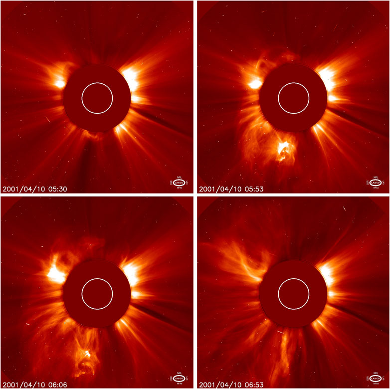
FIGURE 1. Time evolution of a CME, which occurred on 10 April 2001. Images were taken from https://soho.nascom.nasa.gov.
CMEs are often accompanied with solar flares (Priest and Forbes, 2002; Daglis et al., 2004; Chen et al., 2019; Liu et al., 2019; Jiao et al., 2020; Wang et al., 2020; Abduallah et al., 2021; Sun et al., 2022), though the relationship between CMEs and flares is still under active investigation (Yashiro and Gopalswamy, 2008; Kawabata et al., 2018; Liu et al., 2020a; Raheem et al., 2021). Everyday magnetically active regions on the surface of the Sun undergo various changes to cause CMEs, which in turn travel in the interplanetary environment sometimes causing shock waves within and are an important factor for space weather forecasting and other related studies. Any examination in regards to the Sun-based peculiarities, including yet not restricted to these shocks, CMEs and flares, generally requires information connected with the magnetic field of the Sun, their association with one another and the encompassing interplanetary medium. Thus, it is important to show and comprehend the complex magnetic field and its variety regarding time and space. The solar activity encompasses critical elements in the space weather studies. These studies play significant roles for managing satellite tasks, space instrument arrangement and their maintenance as well as climate expectation procedures on Earth. In addition, CMEs are sources of various space weather effects in the near-Earth environment, such as geomagnetic storms. A significant CME can lead to a large-scale, long-term economic and societal catastrophe. Showstack (2013) discussed the potential risks from space weather. The author pointed out that if a geomagnetic storm similar to the Carrington event hit Earth nowadays, it could put up to 40 million Americans at risk of power outages that could last from days to months with tremendous social and economic impacts.
To mitigate the damages that may be caused by CMEs, a large number of methods have been developed to predict the arrival time of CMEs (Zhao and Dryer, 2014; Camporeale, 2019; Vourlidas et al., 2019). Among them, two categories of methods, namely physics-based and machine learning-based, are commonly used. The WSA-ENLIL + Cone (WEC) model (Odstrcil et al., 2004; Riley et al., 2018) is a popular physics-based method for predicting the arrival time of CMEs (Riley et al., 2018). The WEC model has been implemented and used by several organizations including the Space Weather Prediction Center (SWPC) at the National Oceanic and Atmospheric Administration (NOAA) and the Community Coordinated Modeling Center (CCMC) at the NASA Goddard Space Flight Center (GSFC). The WEC model is built by utilizing parameters derived from CME propagation including CME speed, density, location, and propagation direction.
In the category of machine learning methods, Liu et al. (2018) employed a support vector regression (SVR) algorithm to estimate the arrival time of 182 geoeffective CMEs from 1996 to 2015. For each CME, the authors considered related solar wind parameters and CME features obtained from the CME Catalog of the Large Angle and Spectrometric Coronagraph (LASCO) on board SOHO. Wang et al. (2019) designed a convolutional neural network to predict CME arrival time. The authors considered observed images of 223 geoeffective CMEs from 1997 to 2017 where the images were collected from SOHO/LASCO. There were totally 1,122 images with 1–10 images per CME.
In this study, we focus on using machine learning to predict CME transit time, which is the time the body of a CME spends traveling in interplanetary space from the Sun to the Earth. The arrival time can be calculated by adding the transit time to the onset time of the CME. We collect and integrate eruptive events from two solar cycles, #23 and #24, from 1996 to 2021 with a total of 363 geoeffective CMEs. The data used for making predictions include CME features, solar wind parameters and CME images obtained from the SOHO/LASCO C2 coronagraph. Our approach, named CMETNet, is based on an ensemble learning framework, which comprises regression algorithms for numeral/tabular data analysis and a convolutional neural network for image processing. Experimental results demonstrate the good performance of CMETNet, with a Pearson product-moment correlation coefficient of 0.83 and a mean absolute error of 9.75 h.
The rest of this paper is organized as follows. Section 2 describes the data used in this study. Section 3 depicts CMETNet and explains how it works. Section 4 presents experimental results. Section 5 concludes the paper and points out some directions for future research.
Following Liu et al. (2018), we adopted four CME lists: 1) the Richardson and Cane (RC) list (Richardson and Cane, 2010) available at http://www.srl.caltech.edu/ACE/ASC/DATA/level3/icmetable2.htm, 2) the full halo CME list maintained by the University of Science and Technology of China (USTC) (Shen et al., 2014) and available at http://space.ustc.edu.cn/dreams/fhcmes/index.php, 3) the George Mason University (GMU) CME/ICME list (Hess and Zhang, 2017) available at http://solar.gmu.edu/heliophysics/index.php/GMU_CME/ICME_List, and 4) the CME Scoreboard maintained by NASA’s Community Coordinated Modeling Center (CCMC) and available at https://kauai.ccmc.gsfc.nasa.gov/CMEscoreboard/.
We combined and cleaned the CMEs in the four lists based on the procedures described in Liu et al. (2018). We then combined these CMEs from the four lists with those in the catalog presented in Paouris and Mavromichalaki (2017). This process resulted in a set of 363 CMEs from 1996 to 2021. For each of the 363 CMEs, we collected 12 related CME features and solar wind parameters. In addition, for each CME, we downloaded its images from the SOHO/LASCO C2 coronagraph available at https://www.swpc.noaa.gov/products/lasco-coronagraph, as done in Wang et al. (2019). Below, we describe our data integration process in detail.
For each CME list (RC, USTC, GMU, CCMC), we wrote a tracker with Python to automatically gather the onset/appearance times and arrival times of the CMEs in the list. Then, we combined the CMEs in the four lists into a single dataset, removed duplicates and scanned the dataset for events that occurred within the same hour. For the events that occurred within the same hour, we kept only one event among them. Based on the criteria described in Liu et al. (2018), we ended up with 216, 24, 38, and 113 CMEs from the RC, USTC, GMU and CCMC lists respectively. For each collected CME, we kept a record of two parameters: the onset/appearance time of the CME and the arrival time of the CME. In addition to the four CME lists (RC, USTC, GMU, CCMC), we considered the catalog presented in Paouris and Mavromichalaki (2017), which contained 266 CME events. We combined these 266 events with the 216, 24, 38, and 113 CMEs from the RC, USTC, GMU and CCMC lists respectively, and kept only one event among those that occurred within the same hour in our dataset.
This data integration process resulted in 363 geoeffective CMEs. Figure 2 shows the number of CMEs in each year. Solar cycle 23 (1996–2008) has 240 CMEs while solar cycle 24 (2008–late 2019) has 118 CMEs. (There are 5 CMEs between late 2019 and 2021, totaling 363 CMEs between 1996 and 2021 considered in the study.) In solar cycle 23, year 2001 has the most CMEs with 41 CMEs in this year. In solar cycle 24, year 2014 has the most CMEs with 21 CMEs in this year. Years 2007, 2008, 2009, and 2019 have the fewest CMEs with only one CME in each of the 4 years. It is worth mentioning that the CME peak times (i.e., 2001 in solar cycle 23 and 2014 in solar cycle 24) are consistent with the sunspot peak times in the two solar cycles (Raheem et al., 2021). Figure 3 shows the distribution of CME transit times for the 363 events in our dataset. For the 363 CME events, the smallest transit time is 18 h while the largest transit time is 138 h.
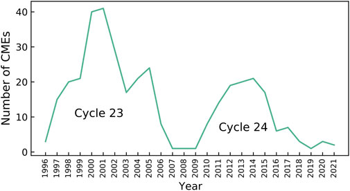
FIGURE 2. Annual counts of the CMEs considered in this study. These CMEs occurred between August 1996 and May 2021. Solar cycle 23 (1996–2008) has more CMEs than solar cycle 24 (2008–late 2019).
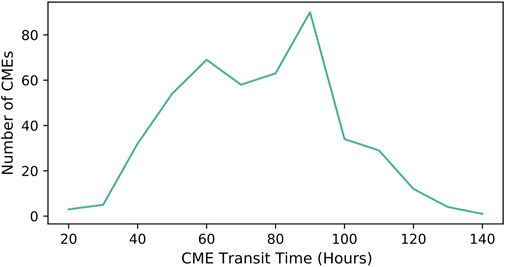
FIGURE 3. Distribution of the transit times of the CMEs considered in this study. For the CMEs, the smallest transit time is 18 h while the largest transit time is 138 h.
For each event in our dataset, we obtained its five features from the SOHO LASCO CME Catalog available at https://cdaw.gsfc.nasa.gov/CME_list/index.html and maintained by the Coordinated Data Analysis Workshops (CDAW) Data Center at NASA (Gopalswamy et al., 2009). The five CME features include angular width, main position angle (MPA), linear speed, 2nd-order speed at final height, and mass. Specifically, for each event in our dataset, by using its onset/appearance time as the key, we retrieved its five features from the LASCO CME Catalog and merged the features with the arrival time of the event in our dataset. For an event E in the dataset whose onset/appearance time does not match the onset/appearance time of any CME in the LASCO CME Catalog, we selected the five features of the temporally closest matching event in the LASCO CME Catalog that occurred within 1 h of E and assigned the five features to E. In the LASCO CME Catalog, a feature F might have a missing value, and the missing value was carried over into our dataset. We employed a data imputation technique by calculating the mean of the available values for the feature F in our dataset and used the mean to represent the missing value.
To obtain the solar wind parameters of each event in our dataset, we followed the approach described in Liu et al. (2018) and used the hourly average data extracted from NASA’s OMNIWeb at https://omniweb.gsfc.nasa.gov/. We considered seven solar wind parameters: Bx, Bz, alpha to proton ratio, flow longitude, plasma pressure, flow speed, and proton temperature. For each event E in our dataset, we used E’s onset/appearance time t as the key, retrieved the solar wind parameter values at timestamp t + 6 (with hourly average resolution) from OMNIWeb, and assigned the retrieved solar wind parameter values to the event E.
In addition to the five CME features and seven solar wind parameters, we downloaded each event’s FITS images from the SOHO/LASCO C2 coronagraph. We were not able to locate the FITS images for 9 out of the 363 events. (For these 9 events, we only considered their CME features and solar wind parameters when training and testing our CMETNet framework.) We followed the approach described in Wang et al. (2019) to match each event in our dataset with the corresponding FITS files in LASCO. Specifically, for each event in our dataset, we downloaded FITS files during the period that is between 10 min before the onset/appearance time of the event and up to 2 h after the event. The Astropy Python package (Astropy Collaboration et al., 2013) was used to read each FITS file and produce a CME image as a 2-dimensional (2D) array. Image sizes in our dataset are: 1,024 × 1,024 pixels, 512 × 512 pixels, or 256 × 256 pixels. For consistency, we reduced the size of all images to 256 × 256 pixels. Images with low quality were discarded. In this way, we obtained a total of 2,281 images with 0–17 images per event.
Finally, we obtained the transit time for a CME event by calculating the difference in hours between the onset/appearance time of the event and the arrival time of the event. For the 363 geoeffective CMEs in our dataset, their transit time ranges from 18 h to approximately 5 days (Figure 3). In other words, the traveling of the CMEs in space from the Sun to the Earth takes between 18 h and approximately 5 days after their first appearance in LASCO.
We adopt an ensemble learning approach to predicting CME transit time. This approach uses a set of machine learning models whose individual predictions are combined to make a final prediction (Dietterich, 2000). An ensemble method is often more accurate than the individual machine learning models that form the ensemble method (Dietterich, 2000). There are several techniques for constructing an ensemble. In this work, we use bootstrap aggregation, or bagging for short, originally proposed by Breiman (1996), which works as follows:
1) Randomly select N training samples with replacement from a given training set with M samples.
2) Repeat step (1) to generate L training subsets, N1, N2, … , NL, where L is the number of learners forming the ensemble method. Notice that the same sample may appear multiple times in the training subsets.
3) Each learner out of the L learners is trained individually and separately by one of the training subsets, N1, N2, …, NL, with no two learners being trained by the same training subset.
4) Each trained learner makes a prediction on a given test sample. The ensemble method produces a final prediction on the test sample through a combination method, which usually works by taking the average of the L predictions made by the L trained learners.
Our ensemble learning framework, named CMETNet and illustrated in Figure 4, comprises five base learners: 1) A support vector regression (SVR) algorithm (Cortes and Vapnik, 1995), 2) a random forest (RF) algorithm (Breiman, 2001), 3) a Gaussian process (GP) algorithm (Yuan et al., 2008), 4) an XGBoost (XGB) algorithm (Chen and Guestrin, 2016), and 5) a convolutional neural network (CNN) (LeCun et al., 1999). The first four learners are regression algorithms used for analyzing the numeral/tabular data related to the CME features and solar wind parameters considered in the study. These four regression algorithms are commonly used in heliophysics and space weather research (Liu et al., 2017; Gruet et al., 2018; Inceoglu et al., 2018; Tang et al., 2021; Abduallah et al., 2022). The fifth learner is a CNN model used for CME image processing. Below, we describe the five base learners and the ensemble method that combines the learners.
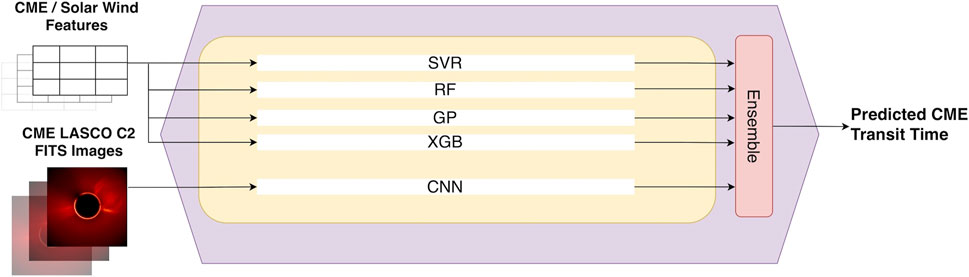
FIGURE 4. Illustration of our CMETNet framework. The framework consists of five machine learning-based regression models: SVR, RF, GP, XGB and CNN. For a CME event E, the first four models (SVR, RF, GP, XGB) accept E’s CME features and solar wind parameters as input while the fifth model (CNN) accepts E’s CME images as input. The five regression models are followed by an ensemble method, which combines the results from the five models and produces the predicted transit time of E.
Our SVR model is taken from the Sklearn library in Python (Pedregosa et al., 2011). We performed parameter tuning to find the optimal hyperparameters of the SVR model by utilizing the GridSearchCV function in Sklearn. We used the Radial Basis Function (RBF) kernel and set the kernel cache size to 200. Our RF algorithm operates by constructing multiple decision trees during training and outputting the mean of the predictions made by the multiple trees during testing. We implemented the RF model using Sklearn and optimized the model parameters by utilizing Sklearn’s RandomizedSearchCV function. The number of trees was set to 800 and the number of attributes used to split a node in a tree was set to the square root of the total number of attributes (which is 12 including the five CME features and seven solar wind parameters used in the study). GP is a non-parametric model that performs data regression using the prior of a Gaussian process. It is a probabilistic approach that provides a level of confidence for the predicted outcome (Görtler et al., 2019). We implemented the GP model using Sklearn with two kernels: Whitekernel and RBF. A noise of 0.5 was used as a parameter for the Whitekernel. XGB is a scalable tree boosting system. We implemented our XGB model by utilizing the XGBoost package presented in Chen and Guestrin (2016). The XGBRegressor class was imported into our CMETNet framework from the XGBoost package with default parameters.
Figure 5 illustrates the architecture of our CNN model. This model is used to predict the CME transit time for an input CMELASCO C2 image. The model starts with a 2D convolutional layer with 64 filters of size 11 × 11 and 1 stride, followed by a Leaky Rectified Linear Unit (LeakyReLU) layer. The output of the LeakyReLU layer is then sent to five convolutional blocks. Each convolutional block contains a 2D convolutional layer with F filters where F = 64, 128, 128, 256, 256 respectively and S strides where S = 2, 1, 2, 1, 2 respectively and the filter size K = 11 × 11. The 2D convolutional layer is followed by a batch normalization layer, which is followed by a LeakyReLU layer. The output feature map of the last convolutional block is sent to two dense layers with 1,024 neurons and 1 neuron, respectively. Finally, the model outputs the transit time by using a linear activation function. The regression loss function used by the CNN model is the mean absolute error (MAE) loss function (Berk, 1992). In training the CNN model, we adopt the adaptive moment estimation (Adam) optimizer (Goodfellow et al., 2016) to find the optimal parameters/weights of the model. Please note that the CNN model predicts the transit time from a single CME image as illustrated in Figure 5. On the other hand, our CMETNet framework takes all the images associated with a CME event, processing and combining the multiple transit times predicted by the CNN model in CMETNet using our ensemble learning method as illustrated in Figure 4 to produce the final, predicted transit time of the CME event. Section 3.3 below details the ensemble learning method.
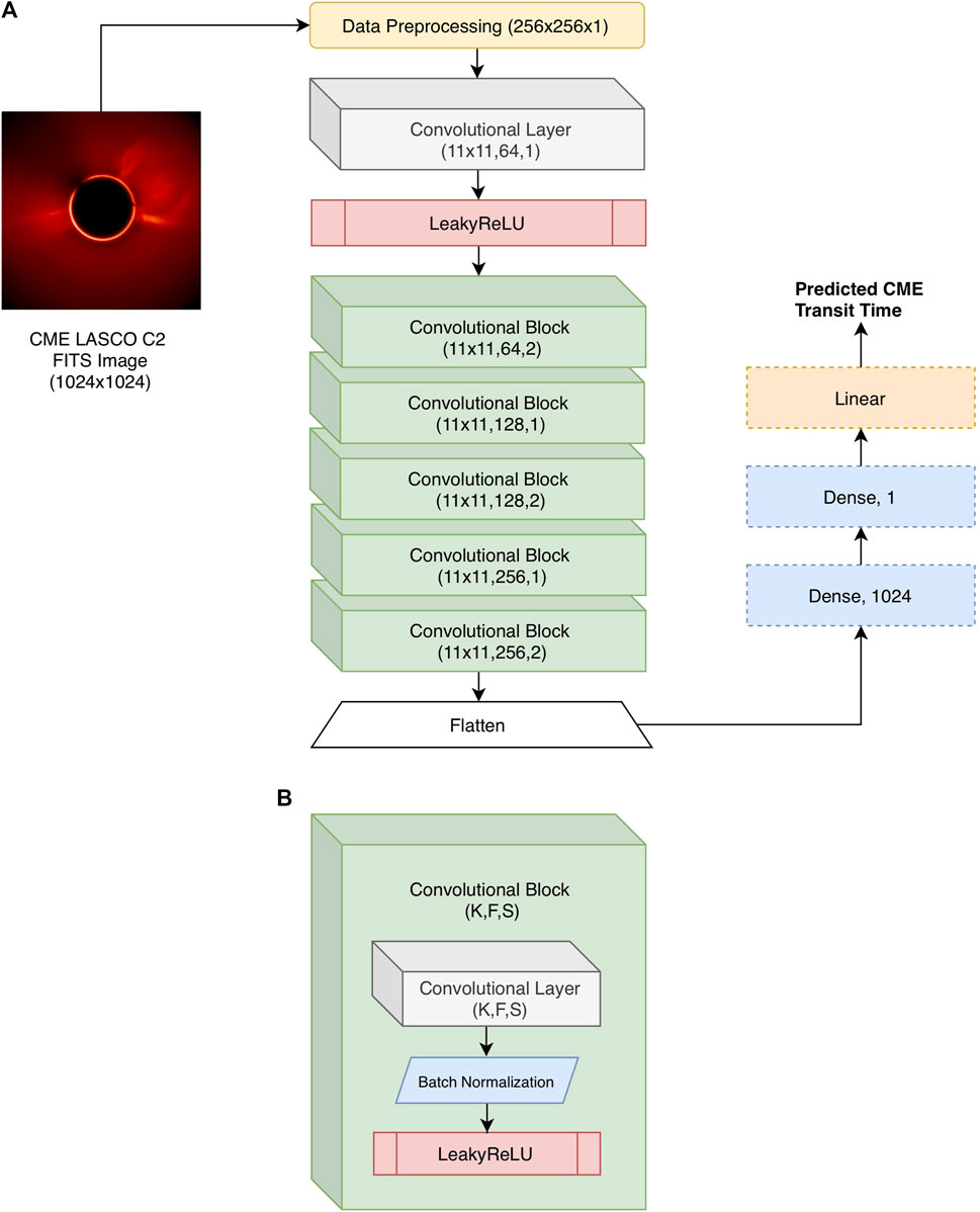
FIGURE 5. Illustration of the CNN model in CMETNet where the CNN model is used to predict the CME transit time for an input CME LASCO C2 image. (A) Overall architecture of the CNN model. The model starts with a 2D convolutional layer with 64 filters of size 11 × 11 and 1 stride, followed by a Leaky Rectified Linear Unit (LeakyReLU) layer. The output of the LeakyReLU layer is then sent to five convolutional blocks. The output feature map of the last convolutional block is sent to two dense layers with 1,024 neurons and 1 neuron, respectively. Finally, the model outputs the predicted CME transit time by using a linear activation function. (B) Detailed configuration of a convolutional block. The convolutional block contains a 2D convolutional layer with F filters where F = 64, 128, 128, 256, 256 respectively and S strides where S = 2, 1, 2, 1, 2 respectively and the filter size K = 11 × 11. The 2D convolutional layer is followed by a batch normalization layer, which is followed by a LeakyReLU layer.
We adapt the original bagging method described in Section 3.1 into the CMETNet framework. Let Tr denote the training set and let Tt denote the test set. Our dataset contains both numerical/tabular data including CME features and solar wind parameters, which are handled by the regression algorithms, and CME images, which are handled by the CNN model. We describe the training procedures for the regression algorithms and the CNN model separately.
For the regression algorithms, we execute the following steps during training.
1) Randomly select 200 training samples with replacement from Tr. Each sample corresponds to a CME event.
2) Repeat step (1) to generate four different training subsets, N1, N2, N3, N4. Note that the same sample may appear multiple times in the training subsets. We also obtain four corresponding validation sets V1, V2, V3, V4 where Vi = Tr − Ni, 1 ≤ i ≤ 4. Each sample in a validation set also corresponds to a CME event.
3) Each of the base learners/regression algorithms, SVR, RF, GP, XGB, is trained individually and separately by one of the training subsets, N1, N2, N3, N4, with no two learners being trained by the same training subset. Each trained learner predicts the transit time of each sample taken from the corresponding validation set. The prediction accuracy on the corresponding validation set is measured by the mean absolute error (MAE) (Berk, 1992).
4) Repeat steps (1) to (3) 100 times to find, for each base learner, the best training subset/model that yields the highest prediction accuracy on the corresponding validation set. Save the best model for each of the four base learners.
Since the four base learners SVR, RF, GP, XGB work on numerical/tabular data only, the data used in the steps (1) to (4) above for the four base learners are the CME features and solar wind parameters associated with each sample/CME event.
Separately, we train the CNN model in a slightly different way. Here, each sample corresponds to a CME image rather than a CME event. A CME event may have multiple images, all of which have the same CME transit time. Thus, we label these multiple CME images/samples with the same CME transit time. We then execute the following steps during training.
1) Randomly select 10% of the samples/CME images in the training set Tr and assign the selected samples into the validation set V.
2) Use the remaining 90% training samples in Tr along with the 10% validation samples in V to train our CNN model. The validation set V is used to find the optimal parameters and hyperparameters to get the best CNN model.
After the training is completed, we obtain the best SVR, RF, GP, XGB, CNN models. During testing, we predict the transit time of each test CME event E in the test set Tt based on the following two cases.
• E does not have CME images. In this case, E only has numerical/tabular data including CME features and solar wind parameters. Then the predicted transit time for E is the median of the transit times predicted by the four regression models SVR, RF, GP, XGB respectively based on E’s CME features and solar wind parameters.
• E has CME images, CME features and solar wind parameters. Without loss of generality, we assume E has k CME images. Then, for each CME image, we use the CNN model to predict the transit time t1 of the image. In addition, we obtain four transit times t2, t3, t4, t5 predicted by the four regression models SVR, RF, GP, XGB respectively based on E’s CME features and solar wind parameters. We take the median of the five predicted transit times t1, t2, t3, t4, t5. E has k CME images, so we obtain k medians. Finally, we take the median of the k medians, which is E’s predicted transit time produced by our ensemble method (CMETNet).
The CME Scoreboard maintained by NASA’s Community Coordinated Modeling Center (CCMC) was launched in 2013. Our dataset contains 363 CMEs that occurred between 1996 and 2021. To compare the predictions produced by our CMETNet and those on the CME Scoreboard, we conducted a 9-fold cross validation experiment as follows. In each run, data in a year between 2013 and 2021 were used as test data, and all the other data together were used as training data. There are 9 years between 2013 and 2021, and hence we had 9 runs/folds. In each run, the test set and training set were disjoint. The prediction accuracy in each run was calculated and the mean and standard deviation over the 9 runs were plotted.
We adopt two evaluation metrics to quantify the performance of a predictive model. The first metric is the mean absolute error (MAE; Berk, 1992), defined as:
Here N denotes the number of CMEs in a test set, and yi (
The second evaluation metric is the Pearson product-moment correlation coefficient (PPMCC; Pearson, 1895), defined as:
Here X and Y represent the actual transit times and predicted transit times in the test set; μX and μY are the mean of X and Y, respectively; σX and σY are the standard deviation of X and Y respectively; and E (⋅) is the expectation. The value of the PPMCC ranges from −1 to 1. A value of 1 means that there is a linear equation relationship between X and Y, where Y increases as X increases. A value of −1 means that all data points lie on a line for which Y decreases as X increases. A value of zero means that there is no linear correlation between the variables X and Y (Liu et al., 2020a).
In this subsection, we performed ablation tests to analyze and evaluate the components of our CMETNet framework. We considered five subunits from CMETNet: SVR, RF, GP, XGB and CNN. In addition, we considered COMB, which was the ensemble of SVR, RF, GP and XGB. That is, COMB was obtained by removing CNN from CMETNet. Figure 6 presents the PPMCC and MAE results of the seven methods: SVR, RF, GP, XGB, CNN, COMB, and CMETNet. In the figure, each colored bar represents the mean over the 9 runs and its associated error bar represents the standard deviation divided by 3 (i.e., the square root of the number of runs) (Iong et al., 2022). It can be seen from Figure 6 that CMETNet achieves the best performance among the seven methods. CMETNet yields better results than COMB, indicating the importance of including the CNN model in our framework. The results based on PPMCC and MAE are consistent.
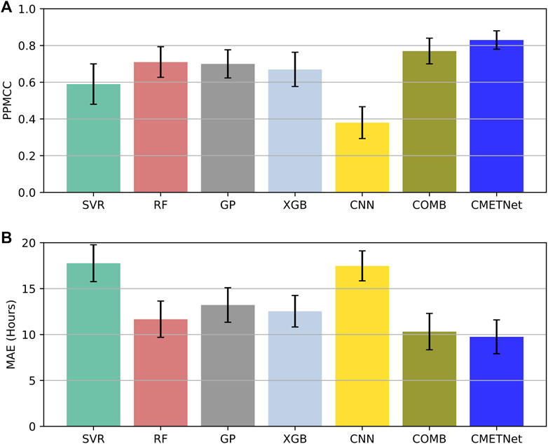
FIGURE 6. Results of the ablation tests for assessing the components (SVR, RF, GP, XGB, CNN) of CMETNet where COMB is the ensemble model of SVR, RF, GP and XGB. (A) Pearson product-moment correlation coefficients (PPMCCs) of the tested models. (B) Mean absolute errors (MAEs) of the tested models. CMETNet achieves the best performance among all the tested models.
Each event E in our dataset has 5 CME features (denoted by F), 7 solar wind parameters (denoted by W) and 0–17 CME images (denoted by I). To evaluate the effectiveness of these features, parameters and images, we performed an additional experiment in which we considered the following seven cases:
• E contains all of the CME features, solar wind parameters and CME images (denoted by FWI);
• E contains only the CME features and solar wind parameters (denoted by FW);
• E contains only the CME features and CME images (denoted by FI);
• E contains only the solar wind parameters and CME images (denoted by WI);
• E contains only the CME features (denoted by F);
• E contains only the solar wind parameters (denoted by W);
• E contains only the CME images (denoted by I).
In each case, we applied CMETNet to the data at hand. Notice that FWI is equivalent to CMETNet. In the FW case, CMETNet amounts to the aforementioned COMB model. In the I case, CMETNet amounts to the aforementioned CNN model.
Figure 7 presents the PPMCC and MAE results of the seven cases. It can be seen from Figure 7 that FWI yields the most accurate results with a PPMCC of 0.83 and an MAE of 9.75 h, indicating that combining the three types of data (CME features, solar wind parameters and CME images) together leads to the best performance. When considering only two types of data together, FI has the highest PPMCC of 0.80; on the other hand, FW yields the best MAE of 10.32 h. When the three types of data are used individually and separately, F yields the best results in terms of both of the two evaluation metrics with a PPMCC of 0.78 and an MAE of 11.39 h. Thus, the CME features have higher predictive power than the solar wind parameters and CME images respectively.
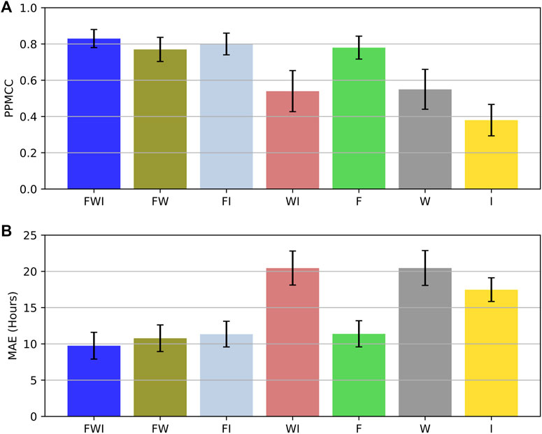
FIGURE 7. Results of the ablation tests for assessing seven cases (FWI, FW, FI, WI, F, W, I) where FWI represents the combination of CME features, solar wind parameters and CME images, FW represents the combination of CME features and solar wind parameters, FI represents the combination of CME features and CME images, WI represents the combination of solar wind parameters and CME images, F represents the CME features, W represents the solar wind parameters, and I represents the CME images. (A) Pearson product-moment correlation coefficients (PPMCCs) of the tested cases. (B) Mean absolute errors (MAEs) of the tested cases. FWI yields the best performance among all the tested cases.
In this experiment, we compared CMETNet with previously published machine learning methods for CME arrival time prediction. Liu et al. (2018) developed an SVR-based method by utilizing the CME features and solar wind parameters considered here. Their method adopted the same SVR model as the one in CMETNet. We represent their method simply as SVR. Wang et al. (2019) developed a CNN model by utilizing the CME images considered here. Their CNN model is different from the CNN model used in CMETNet. We represent their CNN model as PCNN (denoting the Previous CNN). It should be pointed out that, although the features/parameters and images used by SVR and PCNN respectively are the same as those used by CMETNet, the datasets presented in this work are much larger and more comprehensive than those presented in the previous studies (Liu et al., 2018; Wang et al., 2019). As a consequence, the prediction results reported here are not exactly the same as those given in Liu et al. (2018) and Wang et al. (2019).
In addition, we compared CMETNet with three physics-based models, including 1) the WSA-ENLIL + Cone (WEC) model (Odstrcil et al., 2004; Riley et al., 2018) implemented by the Space Weather Prediction Center at the National Oceanic and Atmospheric Administration (NOAA), denoted by WECNOAA; 2) the model available at https://www.sidc.be/developed by the Solar Influences Data Analysis Center (SIDC) at the Royal Observatory of Belgium, denoted by SIDC; and 3) the WSA-ENLIL + Cone (WEC) model implemented by the Community Coordinated Modeling Center (CCMC) at the NASA Goddard Space Flight Center (GSFC), denoted by WECGSFC. These three physics-based models are considered as the best physical models with most accurate prediction results submitted to NASA’s CCMC CME Scoreboard at https://kauai.ccmc.gsfc.nasa.gov/CMEscoreboard/(Riley et al., 2018).
Figure 8 presents the PPMCC and MAE results of the six methods: SVR, PCNN, WECNOAA, SIDC, WECGSFC and CMETNet. Overall, CMETNet yields the most accurate results with a PPMCC of 0.83 and an MAE of 9.75 h. Among the three physics-based methods, WECNOAA has the highest PPMCC of 0.79 while WECGSFC has the lowest MAE of 11.49 h. Both CMETNet and the three physics-based methods perform better than the previously published machine learning methods SVR and PCNN (Liu et al., 2018; Wang et al., 2019).
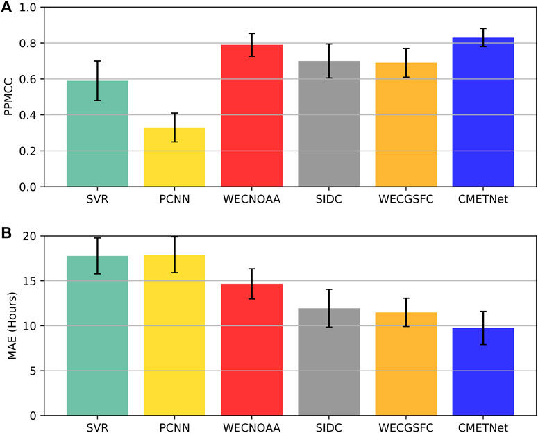
FIGURE 8. Performance comparison of six methods for CME arrival time prediction. CMETNet is the ensemble learning framework proposed in this paper. SVR and PCNN are previously published machine learning methods. WECNOAA, SIDC, and WECGSFC are physics-based models presented on NASA’s CCMC CME Scoreboard. (A) Pearson product-moment correlation coefficients (PPMCCs) of the six methods. (B) Mean absolute errors (MAEs) of the six methods. CMETNet outperforms the other five methods in terms of both PPMCC and MAE.
Supplementary Table S1 in the Supplementary Material further compares the performance of CMETNet and the three physics-based methods. Each number in the table represents the actual CME transit time minus the predicted CME transit time. Thus, a positive number means that the actual CME transit time is greater than the predicted CME transit time while a negative number means that the actual CME transit time is smaller than the predicted CME transit time. For each CME, the boldfaced number with the smallest absolute value represents the best prediction result among those predicted by the four methods. The “−” symbol indicates that there is no record for the corresponding method on NASA’s CCMC CME Scoreboard. The results in Supplementary Table S1 are consistent with those in Figure 8, showing CMETNet outperforms the three physics-based methods.
In this paper we presented an ensemble framework (CMETNet) for predicting the arrival time of CME events. Each event contains 5 CME features (angular width, main position angle, linear speed, 2nd-order speed at final height, and mass), 7 solar wind parameters (Bx, Bz, alpha to proton ratio, flow longitude, plasma pressure, flow speed, and proton temperature) and 0–17 CME images. The CMETNet framework is composed of five machine learning models including support vector regression (SVR), random forest (RF), Gaussian process (GP), XGBoost (XGB), and a convolutional neural network (CNN). Our experimental results demonstrated that CMETNet outperforms the individual machine learning models with a PPMCC of 0.83 and an MAE of 9.75 h. Furthermore, using all the CME features, solar wind parameters and CME images together yields better performance than using part of them.
We then compared CMETNet with two previously published machine learning methods (Liu et al., 2018; Wang et al., 2019) and three physics-based methods (WECNOAA, SIDC, and WECGSFC). These three physics-based methods are considered as the best physical models with most accurate prediction results submitted to NASA’s CCMC CME Scoreboard. Our experimental results showed that both CMETNet and the three physics-based methods produce more accurate results than the two previously published machine learning methods, with CMETNet achieving the best performance among all the methods.
The success of CMETNet is attributed to the integration of data from multiple sources and combination of multiple machine learning models. Nevertheless, accurately predicting CME arrival time remains a challenging task as the MAE of CMETNet (9.75 h) is still large, indicating there is much room to improve. One possible way for improving the performance of the predictive model is to combine machine learning with physics-based methods as done in a recent study (Tiwari et al., 2021). Dumbović et al. (2021) reviewed several physical drag-based model (DBM) tools for predicting CME arrival time and speed. In future work we plan to explore the combinations of these DBM tools and different machine learning models for more accurate CME arrival time prediction.
Another direction for future research is to develop an operational near real-time CME arrival time prediction system using machine learning. CME features and solar wind parameters are not applicable here since they are not availabe in real time. We plan to predict the transit times of CMEs, right after a CME occurred and was caught on LASCO C2 images (https://www.swpc.noaa.gov/products/lasco-coronagraph) or STEREO COR2 (https://stereo-ssc.nascom.nasa.gov/browse/), which can be obtained within a few hours. This near real-time prediction system will require new, advanced CNN models to learn latent features or representations from the CME images. More research is needed to develop such advanced CNN models.
The original contributions presented in the study are included in the article/Supplementary Material, further inquiries can be directed to the corresponding author.
JW and HW conceived of the study. KA, YA, and HJ implemented the machine learning methods. KA, JW, HW, and YX collected the data and designed the experiments. All of the authors participated in the discussion of the results, co-wrote the paper, and approved its final version.
This work was supported by U.S. NSF grants AGS-1927578, AGS-1954737, and AGS-2149748.
We thank the reviewers for very helpful and thoughtful comments. We also thank Jie Zhang of George Mason University for his assistance in obtaining CME LASCO C2 images. The solar wind data is provided by NASA’s Goddard Space Physics Data Facility. The SOHO LASCO CME Catalog is created and maintained by NASA’s CDAW Data Center and the Catholic University of America in cooperation with the Naval Research Laboratory. SOHO is a project of international cooperation between ESA and NASA.
The authors declare that the research was conducted in the absence of any commercial or financial relationships that could be construed as a potential conflict of interest.
All claims expressed in this article are solely those of the authors and do not necessarily represent those of their affiliated organizations, or those of the publisher, the editors and the reviewers. Any product that may be evaluated in this article, or claim that may be made by its manufacturer, is not guaranteed or endorsed by the publisher.
The Supplementary Material for this article can be found online at: https://www.frontiersin.org/articles/10.3389/fspas.2022.1013345/full#supplementary-material
Abduallah, Y., Jordanova, V. K., Liu, H., Li, Q., Wang, J. T. L., and Wang, H. (2022). Predicting solar energetic particles using SDO/HMI vector magnetic data products and a bidirectional LSTM network. Astrophysical J. Suppl. 260, 16. doi:10.3847/1538-4365/ac5f56
Abduallah, Y., Wang, J. T. L., Nie, Y., Liu, C., and Wang, H. (2021). DeepSun: Machine-learning-as-a-service for solar flare prediction. Res. Astron. Astrophys. 21, 160. doi:10.1088/1674-4527/21/7/160
Astropy Collaboration, Robitaille, T. P., Tollerud, E. J., Greenfield, P., Droettboom, M., Bray, E., Aldcroft, T., et al. (2013). Astropy: A community Python package for astronomy. Astron. Astrophys. 558, A33. doi:10.1051/0004-6361/201322068
Berk, K. N. (1992). Regression analysis (ashish sen and muni srivastava). SIAM Rev. Soc. Ind. Appl. Math. 34, 157–158. doi:10.1137/1034042
Camporeale, E. (2019). The challenge of machine learning in space weather: Nowcasting and forecasting. Space weather. 17, 1166–1207. doi:10.1029/2018SW002061
Chen, T., and Guestrin, C. (2016). “XGBoost: A scalable tree boosting system,” in Proceedings of the 22nd ACM SIGKDD international conference on knowledge discovery and data mining. Editors B. Krishnapuram, M. Shah, A. J. Smola, C. C. Aggarwal, D. Shen, and R. Rastogi (San Francisco, CA, USA: ACM), 785–794. doi:10.1145/2939672.2939785
Chen, Y., Manchester, W. B., Hero, A. O., Toth, G., DuFumier, B., Zhou, T., et al. (2019). Identifying solar flare precursors using time series of SDO/HMI images and SHARP parameters. Space weather. 17, 1404–1426. doi:10.1029/2019SW002214
Cortes, C., and Vapnik, V. (1995). Support-vector networks. Mach. Learn. 20, 273–297. doi:10.1007/BF00994018
Daglis, I., Baker, D., Kappenman, J., Panasyuk, M., and Daly, E. (2004). Effects of space weather on technology infrastructure. Space weather. 2, S02004. doi:10.1029/2003SW000044
Dietterich, T. G. (2000). “Ensemble methods in machine learning,” in Multiple classifier systems, first international workshop, MCS 2000, cagliari, Italy, june 21-23, 2000, proceedings. Editors J. Kittler, and F. Roli (Berlin, Germany: Springer), 1–15. doi:10.1007/3-540-45014-9_1
Dumbović, M., Čalogović, J., Martinić, K., Vršnak, B., Sudar, D., Temmer, M., et al. (2021). Drag-based model (DBM) tools for forecast of coronal mass ejection arrival time and speed. Front. Astron. Space Sci. 8, 58. doi:10.3389/fspas.2021.639986
Goodfellow, I., Bengio, Y., and Courville, A. (2016). Deep learning. Massachusetts, United States: MIT Press.
Gopalswamy, N. (2016). History and development of coronal mass ejections as a key player in solar terrestrial relationship. Geosci. Lett. 3, 8. doi:10.1186/s40562-016-0039-2
Gopalswamy, N., Yashiro, S., Michalek, G., Stenborg, G., Vourlidas, A., Freeland, S., et al. (2009). The SOHO/LASCO CME catalog. Earth Moon Planets 104, 295–313. doi:10.1007/s11038-008-9282-7
Görtler, J., Kehlbeck, R., and Deussen, O. (2019). A visual exploration of Gaussian processes. Distill 4. doi:10.23915/distill.00017
Gruet, M. A., Chandorkar, M., Sicard, A., and Camporeale, E. (2018). Multiple-hour-ahead forecast of the Dst index using a combination of long short-term memory neural network and Gaussian process. Space weather. 16, 1882–1896. doi:10.1029/2018SW001898
Hess, P., and Zhang, J. (2017). A study of the Earth-affecting CMEs of solar cycle 24. Sol. Phys. 292, 80. doi:10.1007/s11207-017-1099-y
Inceoglu, F., Jeppesen, J. H., Kongstad, P., Hernández Marcano, N. J., Jacobsen, R. H., and Karoff, C. (2018). Using machine learning methods to forecast if solar flares will be associated with CMEs and SEPs. Astrophys. J. 861, 128. doi:10.3847/1538-4357/aac81e
Iong, D., Chen, Y., Toth, G., Zou, S., Pulkkinen, T. I., Ren, J., et al. (2022). New findings from explainable SYM-H forecasting using gradient boosting machines. Earth Space Sci. Open Archive, 20, e2021SW002928. doi:10.1002/essoar.10508063.3
Jiao, Z., Sun, H., Wang, X., Manchester, W., Gombosi, T., Hero, A., et al. (2020). Solar flare intensity prediction with machine learning models. Space weather. 18, e02440. doi:10.1029/2020SW002440
Kawabata, Y., Iida, Y., Doi, T., Akiyama, S., Yashiro, S., and Shimizu, T. (2018). Statistical relation between solar flares and coronal mass ejections with respect to sigmoidal structures in active regions. Astrophys. J. 869, 99. doi:10.3847/1538-4357/aaebfc
LeCun, Y., Haffner, P., Bottou, L., and Bengio, Y. (1999). “Object recognition with gradient-based learning,” in Shape, contour and grouping in computer vision. Editors D. A. Forsyth, J. L. Mundy, V. D. Gesù, and R. Cipolla (Berlin, Germany: Springer), 319. doi:10.1007/3-540-46805-6_19
Liu, C., Deng, N., Wang, J. T. L., and Wang, H. (2017). Predicting solar flares using SDO/HMI vector magnetic data products and the random forest algorithm. Astrophys. J. 843, 104. doi:10.3847/1538-4357/aa789b
Liu, H., Liu, C., Wang, J. T. L., and Wang, H. (2020a). Predicting coronal mass ejections using SDO/HMI vector magnetic data products and recurrent neural networks. Astrophys. J. 890, 12. doi:10.3847/1538-4357/ab6850
Liu, H., Liu, C., Wang, J. T. L., and Wang, H. (2019). Predicting solar flares using a long short-term memory network. Astrophys. J. 877, 121. doi:10.3847/1538-4357/ab1b3c
Liu, H., Xu, Y., Wang, J., Jing, J., Liu, C., Wang, J. T. L., et al. (2020b). Inferring vector magnetic fields from Stokes profiles of GST/NIRIS using a convolutional neural network. Astrophys. J. 894, 70. doi:10.3847/1538-4357/ab8818
Liu, J., Ye, Y., Shen, C., Wang, Y., and Erdélyi, R. (2018). A new tool for CME arrival time prediction using machine learning algorithms: CAT-PUMA. Astrophys. J. 855, 109. doi:10.3847/1538-4357/aaae69
Maloney, S., Byrne, J., Gallagher, P. T., and McAteer, R. T. J. (2010). The propagation of a CME front in 3D. 38th COSPAR Sci. Assem. 38, 5.
Maloney, S. (2012). Propagation of coronal mass ejections in the inner heliosphere. Ph.D. thesis (Trinity College Dublin: School of Physics).
Odstrcil, D., Riley, P., and Zhao, X. P. (2004). Numerical simulation of the 12 May 1997 interplanetary CME event. J. Geophys. Res. 109. doi:10.1029/2003JA010135
Paouris, E., and Mavromichalaki, H. (2017). Interplanetary coronal mass ejections resulting from Earth-directed CMEs using SOHO and ACE combined data during solar cycle 23. Sol. Phys. 292, 30. doi:10.1007/s11207-017-1050-2
Pearson, K. (1895). Note on regression and inheritance in the case of two parents. Proc. R. Soc. Lond. 58, 240–242. doi:10.1098/rspl.1895.0041
Pedregosa, F., Varoquaux, G., Gramfort, A., Michel, V., Thirion, B., Grisel, O., et al. (2011). Scikit-learn: Machine learning in Python. J. Mach. Learn. Res. 12, 2825–2830. doi:10.5555/1953048.2078195
Priest, E. R., and Forbes, T. G. (2002). The magnetic nature of solar flares. Astron. Astrophys. Rev. 10, 313–377. doi:10.1007/s001590100013
Raheem, A.-u., Cavus, H., Coban, G. C., Kinaci, A. C., Wang, H., and Wang, J. T. L. (2021). An investigation of the causal relationship between sunspot groups and coronal mass ejections by determining source active regions. Mon. Not. R. Astron. Soc. 506, 1916–1926. doi:10.1093/mnras/stab1816
Richardson, I. G., and Cane, H. V. (2010). Near-Earth interplanetary coronal mass ejections during solar cycle 23 (1996 - 2009): Catalog and summary of properties. Sol. Phys. 264, 189–237. doi:10.1007/s11207-010-9568-6
Riley, P., Mays, M. L., Andries, J., Amerstorfer, T., Biesecker, D., Delouille, V., et al. (2018). Forecasting the arrival time of coronal mass ejections: Analysis of the CCMC CME Scoreboard. Space weather. 16, 1245–1260. doi:10.1029/2018SW001962
Schwenn, R., dal Lago, A., Huttunen, E., and Gonzalez, W. D. (2005). The association of coronal mass ejections with their effects near the Earth. Ann. Geophys. 23, 1033–1059. doi:10.5194/angeo-23-1033-2005
Shen, C., Wang, Y., Pan, Z., Miao, B., Ye, P., and Wang, S. (2014). Full-halo coronal mass ejections: Arrival at the Earth. J. Geophys. Res. Space Phys. 119, 5107–5116. doi:10.1002/2014JA020001
Showstack, R. (2013). Experts caution about potential increased risks from space weather. Eos Trans. AGU. 94, 222–223. doi:10.1002/2013EO250003
Sun, Z., Bobra, M. G., Wang, X., Wang, Y., Sun, H., Gombosi, T., et al. (2022). Predicting solar flares using CNN and LSTM on two solar cycles of active region data. Astrophys. J. 931, 163. doi:10.3847/1538-4357/ac64a6
Tang, R., Zeng, X., Chen, Z., Liao, W., Wang, J., Luo, B., et al. (2021). Multiple CNN variants and ensemble learning for sunspot group classification by magnetic type. Astrophys. J. Suppl. Ser. 257, 38. doi:10.3847/1538-4365/ac249f
Tiwari, A., Camporeale, E., Teunissen, J., Foldes, R., Napoletano, G., and Del Moro, D. (2021). Predicting arrival time for CMEs: Machine learning and ensemble methods. Munich, Germany: EGU General Assembly Conference Abstracts, 7661. doi:10.5194/egusphere-egu21-7661
Vourlidas, A., Patsourakos, S., and Savani, N. P. (2019). Predicting the geoeffective properties of coronal mass ejections: Current status, open issues and path forward. Phil. Trans. R. Soc. A 377, 20180096. doi:10.1098/rsta.2018.0096
Wang, X., Chen, Y., Toth, G., Manchester, W. B., Gombosi, T. I., Hero, A. O., et al. (2020). Predicting solar flares with machine learning: Investigating solar cycle dependence. Astrophys. J. 895, 3. doi:10.3847/1538-4357/ab89ac
Wang, Y., Liu, J., Jiang, Y., and Erdélyi, R. (2019). CME arrival time prediction using convolutional neural network. Astrophys. J. 881, 15. doi:10.3847/1538-4357/ab2b3e
Yashiro, S., and Gopalswamy, N. (2008). Statistical relationship between solar flares and coronal mass ejections. Proc. Int. Astron. Union 4, 233–243. doi:10.1017/S1743921309029342
Yuan, J., Wang, K., Yu, T., and Fang, M. (2008). Reliable multi-objective optimization of high-speed WEDM process based on Gaussian process regression. Int. J. Mach. Tools Manuf. 48, 47–60. doi:10.1016/j.ijmachtools.2007.07.011
Keywords: heliophysics, space weather, coronal mass ejections, interplanetary shocks, machine learning
Citation: Alobaid KA, Abduallah Y, Wang JTL, Wang H, Jiang H, Xu Y, Yurchyshyn V, Zhang H, Cavus H and Jing J (2022) Predicting CME arrival time through data integration and ensemble learning. Front. Astron. Space Sci. 9:1013345. doi: 10.3389/fspas.2022.1013345
Received: 06 August 2022; Accepted: 22 September 2022;
Published: 06 October 2022.
Edited by:
Yang Chen, University of Michigan, United StatesReviewed by:
Reinaldo Roberto Rosa, National Institute of Space Research (INPE), BrazilCopyright © 2022 Alobaid, Abduallah, Wang, Wang, Jiang, Xu, Yurchyshyn, Zhang, Cavus and Jing. This is an open-access article distributed under the terms of the Creative Commons Attribution License (CC BY). The use, distribution or reproduction in other forums is permitted, provided the original author(s) and the copyright owner(s) are credited and that the original publication in this journal is cited, in accordance with accepted academic practice. No use, distribution or reproduction is permitted which does not comply with these terms.
*Correspondence: Jason T. L. Wang, d2FuZ2pAbmppdC5lZHU=
Disclaimer: All claims expressed in this article are solely those of the authors and do not necessarily represent those of their affiliated organizations, or those of the publisher, the editors and the reviewers. Any product that may be evaluated in this article or claim that may be made by its manufacturer is not guaranteed or endorsed by the publisher.
Research integrity at Frontiers
Learn more about the work of our research integrity team to safeguard the quality of each article we publish.