Wave-particle interactions toolset: A python-based toolset to model wave-particle interactions in the magnetosphere

Wave particle interactions are known to be an efficient yet unquantified driver of the variability of particle populations in Earth’s magnetosphere, and their quantification and understanding through modelling has been a subject of ceaseless and extensive research during the last decades. Moreover, there is an increasing interest in techniques for radiation belt remediation, which refers to artificially controlling energetic particle populations in the near-Earth space environment via the scattering of particles from artificially generated electromagnetic waves. Whereas numerous modelling techniques are described in literature, there is a lack of a unified open-source toolset that incorporates the equations and parameterizations used by different wave-particle interaction models in a user-friendly environment. We present WPIT, the Wave-Particle Interactions Toolset, an open source, Python-based set of tools for modelling the interactions between energetic charged particles and VLF waves in the magnetosphere through test particle simulations. WPIT incorporates key routines related to wave-particle interactions in Python modules and also in Jupyter Notebook environment, enabling the traceability of all relevant equations in terms of their derivation and key assumptions, together with the programming environment and integrated graphics that enable users to conduct state-of-the-art wave-particle interaction simulations rapidly and efficiently. WPIT can be used either as a stand-alone simulation tool or as a library of routines that the user can extract and incorporate into an independent simulation. We present an analytic description of the code, the methodology used, and examples based on each of the WPIT modules. WPIT examples include the exact reproduction of simulation results that have been reported in literature, based on the same sets of parameters and assumptions, allowing the user to expand upon state-of-the-art. Finally, using the WPIT toolset, we perform a parametric analysis on the onset of nonlinear interactions between electrons with whistler-mode waves by varying the relevant parameters of the waves (amplitude, wave normal angle and frequency), the particles (pitch angle and energy) and the plasma environment (electron density and ion composition).

1 Introduction

1.1 Background on wave-particle interaction modeling in the magnetosphere

The observed variability in the radiation belts is the outcome of an imbalance between a variety of source and loss processes. In the collisionless regime of the magnetosphere the changes in the particle populations are mainly controlled by interactions with a plethora of plasma waves, which may lead to the violation of one or more of the adiabatic invariants (Schulz and Lanzerotti, 2012). Very low frequency (VLF) frequency waves can violate the first and second adiabatic invariants, leading to pitch angle scattering, acceleration and potential loss of particles to the upper atmosphere (Horne and Thorne, 1998; Kivelson, 2005; Shprits, 2009). Resonant wave-particle interactions are an efficient scattering mechanism of energetic particles, leading to pitch angle and energy changes of energetic particles (Koskinen and Kilpua, 2022).

There are several different approaches that are commonly used to simulate wave particle interactions. These are generally classified in three categories, namely quasi linear theory (e.g., see Albert (2005) and Summers (2005)), Particle-In-Cell (PIC) methodology (e.g., see Allanson et al., 2019 and Allanson et al., 2020) and test particle simulations. WPIT focuses on the test particle simulation methodology.

There are two main approaches in the test particle simulation methodology: the first approach is to integrate the Lorentz equations of charged particle motion in order to trace particle trajectories under the effect of the waves while monitoring changes in the particles’ pitch angle and energy, termed here the full Lorentz approach. The second approach is to use the gyro-averaged equations of motion (e.g. Bell, 1984; Jasna et al., 1992; Bortnik 2004; Bortnik et al., 2015; Li et al., 2015). The gyro-averaged approach has the advantage of reducing the system from a six-dimensional space (i.e. x, y, z, u_x, u_y, u_z, or 3R3V space) to a four-dimensional space (i.e. u_‖, u_⊥, z, η, or 2R2V space]). WPIT in its current form implements the gyro-averaged test particle simulation approach.

In an early publication on wave-particle interactions, Laval and Pellat (1970), investigated the acceleration of particles due to interactions with electrostatic waves. They assumed a parallel propagating electrostatic wave with fixed frequency. They concluded that the trapping of particles in an electrostatic wave could account for particle acceleration and regarded this as a potential mechanism for the precipitation of low-energy electrons. Later on, Nunn (1974) investigated the generation of VLF triggered emissions through nonlinear cyclotron resonance interactions between electrons and a narrow band whistler mode wave travelling in a magnetospheric duct (i.e. parallel propagation). Their results indicated that the nonlinear interactions of electrons with a ducted whistler mode wave can account for the generation of triggered emissions. Karpman et al. (1975) presented an analytic formulation for the investigation of the effects of nonlinear interactions between particles and monochromatic waves. Starting their theoretical analysis for Langmuir waves, they extended their formulation to parallel propagating whistler-mode waves. Karpman and Shklyar (1977) calculated particle precipitation caused by interactions of electrons with a coherent whistler-mode wave. It is noted that in the above studies, the wave was assumed to propagate parallel to the magnetic field, thus omitting any potential effects of interactions with an obliquely propagating wave.

The first formulation of wave-particle interactions for non-relativistic electrons under the effect of oblique whistler-mode waves using the gyro-averaged approach was given by Inan and Tkalcevic (1982). Subsequently, Bell (1984) applied a similar methodology to model first-order cyclotron resonant interactions. Ginet and Albert (1991) and Bortnik et al. (2003) generalised Bell’s formulation to account for interactions with relativistic electrons. Li et al. (2015) found that the formulation of Bortnik et al. (2003) lacked a term that led to differences in the perpendicular motion of electrons.

Many studies where performed in the last decades using the test particle approach. For example, Fu et al. (2020) used full Lorentz approach to investigate cyclotron, Landau and bounce resonances of electrons with hiss. Tao et al. (2012) compared diffusion coefficients with test particle results. Chang et al. (2014) used the full Lorentz approach for investigating interactions of electrons with whistlers artificially generated by ionospheric modification. Li et al. (2015) compared their derived gyro-averaged equations with results from the full Lorentz approach, and found that the two approaches lead to fairly similar results, except for small amplitude fluctuations at gyro-frequency timescales. Huang et al. (2017) proposed the crucial role of the initial gyrophase in the acceleration of electrons by low frequency waves. Inan (1987) investigated the interactions of electrons with field-aligned whistler-mode wave packets. Gao et al. (2014) investigated the interaction of electrons with chorus waves. Su et al. (2013) explored interactions of electrons with EMIC waves. Su et al. (2014) addressed interactions of ring current ions with EMIC waves. Shklyar and Matsumoto (2009), in a review paper, presented analytically the theory of resonant interactions between energetic charged particles and an oblique whistler-mode wave in a non-uniform magnetic field and in the inhomogeneous plasma of the magnetosphere. They used a Hamiltonian approach to derive the basic equations for the wave field and for the particle dynamics. They applied their formulation on two applications: they fisrt calculated the damping (or growth) of an oblique whistler wave and subsequently they used their formulation to calculate proton precipitation by ground-based VLF transmitters. In a review paper, Albert et al. (2012) derived gyro-averaged equations both directly from the full Lorentz equations, as well as through a Hamiltonian approach, accounting for relativistic particles and oblique waves in their formulations. One key result from that study is that the Hamiltonian approach manages to reduce the system to a ‘1 1/2’ dimension, allowing the development of analytical treatments of the change in pitch angle due to resonant interactions with whistler-mode waves.

An important aspect of wave-particle interactions is the appearance of nonlinear effects, which may lead to large pitch angle scattering and energy change for a subset of the particle population undergoing wave-particle interactions. Several studies have focused on identifying nonlinear effects by utilising test particle simulations: Nunn and Omura (2015) explored nonlinear effects in VLF wave fields. Liu et al. (2012) investigated phase bunching and phase trapping effects in interactions of electrons with EMIC waves of large amplitude. Artemyev et al. (2013) compared the importance of Landau vs. cyclotron resonances for nonlinear effects in interactions of electrons with oblique whistler waves. Bortnik et al. (2008) investigated the behaviour of electrons interacting with large amplitude chorus waves. Albert and Bortnik (2009) addressed the rapid loss of radiation belt electrons during geomagnetic storms with test particle simulations under the effect of large amplitude EMIC waves. Gan et al. (2020) explored the effects of wave amplitude modulation in nonlinear electron-chorus interactions. Tao and Bortnik (2010) derived a map of probable regions where nonlinear interactions could be expected. Wang et al. (2019) and Wang et al. (2016) explored nonlinear interactions of EMIC waves with electrons, whereas Lee et al. (2020) focused on interactions of EMIC waves with 90° pitch angle electrons. Bell (1986) calculated the minimum threshold in terms of wave amplitude for nonlinear effects to occur. Artemyev et al. (2020) and Vainchtein et al. (2018) used Hamiltonian theory to address nonlinear wave particle interactions and explore the evolution of electron distributions.

The aforementioned studies constitute only a small subset of the available literature on test particle simulations of wave-particle interactions, however it is often the case that the underlying code that implements the various approximations and equations that are used is not readily available. Furthermore, inter-comparisons between the various methods and the sensitivity to a different set of initial conditions can not be easily implemented. WPIT addresses this gap by providing a python-based, user-friendly toolset of routines that simulate wave-particle interactions in the Earth’s magnetosphere under various models and assumptions proposed in literature and for a range of user-defined environment, wave and particle conditions.

1.2 Overview of WPIT

WPIT is composed in Python, in four different modules as described in the following section. The source code of each of the four modules is accompanied by corresponding Jupyter Notebook, that combines in a comprehensive way the corresponding code, the underlying equations and theory, the output of computations performed by the code, and visualizations of the code results, along with explanatory text on the usage of the underlying code. An advantage of Jupyter Notebooks is that all the above are provided in a single document, allowing scientists to easily access all elements of the programming process while tracing the methodology that is being implemented to its source in literature.

In the remainder of this paper, the methodology employed by each module is described in Section 2, including a brief description of the code. Examples from the use of WPIT are included in Section 3, including usage limitations. Finally, the scalability of WPIT and potential other uses are described in Section 4, including, but not limited to, its potential application for theoretical studies of wave particle interactions, missions targeting wave-particle interaction experiments and investigations on the efficiency of radiation belt remediation techniques.

1.3 WPIT repository and structure

An overview of the WPIT repository is presented in Figure 1. In this figure, WPIT Repo represents the WPIT repository, which is publicly available and can be found at: https://github.com/stourgai/WPIT. Within the repository, the WPIT folder, marked in yellow in Figure 1, contains the source code that is built in the form of four main modules. These are: (a) Environment_mod, used to setup the environment parameters for each simulation; (b) WaveProperties_mod, used to define the properties of the waves; (c) the LandauDamp_mod, which calculates the attenuation of waves according to the Landau damping theory; and (d) WPI_mod, within which the actual wave-particle interactions are implemented. WPI_mod includes three sub-modules, implementing different types of wave-particle interactions, under the effect of oblique whistler mode waves, oblique EMIC waves and parallel EMIC waves, as marked. Each of the modules will be described in further detail in the following sections. The Module_descriptions folder contains Jupyter notebooks with analytic theoretical descriptions of the equations used by each of the four modules described above, along with samples for calling each routine. The WPIT_tests folder contains a set of WPIT implementations that aim to reproduce results found in literature. These are written in Jupyter notebooks, and act as a verification of the code and as tutorials of the use of WPIT. The WPIT_Results folder contains the Jupyter notebooks of the simulations presented in Section 4. Finally, the Documentation folder includes the API documentation of the source code in .html format.

FIGURE 1

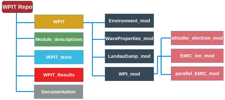
FIGURE 1. A schematic of the organization and contents of the WPIT repository.

2 Methods

The code comprising WPIT is formatted in Python modules with specific applications as described below, and is accompanied by Jupyter notebooks, whereby the code is complemented by references to the equations and methods used and where examples can be plotted as direct outputs of the calculations performed. The WPIT source code can be found at: https://github.com/stourgai/WPIT/tree/main/WPIT. The code has been tested on Ubuntu 18.04, Intel Core i7, 2.6 GHz and 16 GB RAM.

As an example of the processing time and the computational resources needed for integrations of particle trajectories under the effect of waves, it is noted that in the machines used for testing of the code as discussed above, the simulation of the resonant interactions of a wave with a 45° pitch angle electron at L = 5 and with energy of 500 over one bounce period requires a real time of computation of approximately 30 s. The wave in the simulation is assumed to be present at every step of the particle trajectory, thus the wave characteristics are calculated at every time-step. A Jupyter notebook of the simulation is available in WPIT_results folder of the WPIT repository (WPIT_Computational_Time.ipynb). It is noted that this computation time is only indicative, and is dependent on particle parameters, and primarily on the particle’s pitch angle; it is also noted that the computation time scales linearly with the total number of bounce periods.

In the following we outline the functionality of each of the modules comprising WPIT.

2.1 Environment characterization module

Module WPIT. Environment_mod includes routines for the calculation of environment parameters that are needed for wave particle interaction simulations. The routines of the of module are listed in Table 1. These include routines for the calculation of: the geomagnetic field, the electron density through various models including the models by Carpenter and Anderson (1992), Sheeley et al. (2001), Denton et al. (2002) and Ozhogin et al. (2012), the particle gyro-frequency, the plasma frequency, the upper and lower hybrid frequencies, the gradients of the gyro-frequency and the strength of the magnetic field along a magnetic field line, the L-shell, the bounce and drift periods, equatorial pitch angle mapping, the Larmor radius, the first adiabatic invariant, the bounce loss cone angle, the Debye length, and a routine to calculate particle velocity from a particle’s energy and local pitch angle. Moreover, this module includes the WPIT. Environment_mod.const routine which sets all the constants that are needed for the simulations. Detailed description of each routine along with example runs can be found in the Environment_mod_description Jupyter notebook, located in the Module_descriptions folder of the WPIT repository.

TABLE 1

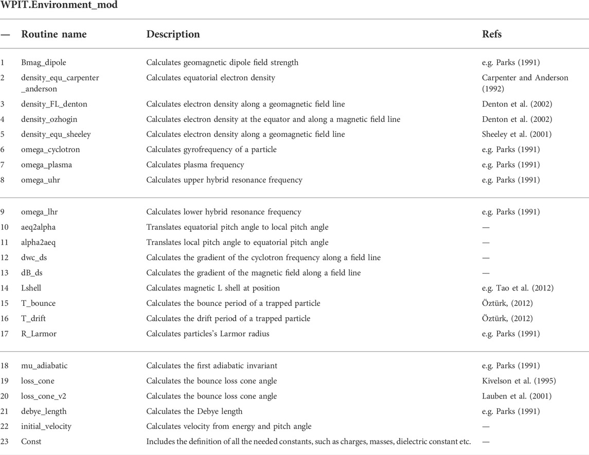
TABLE 1. Environment module routines.

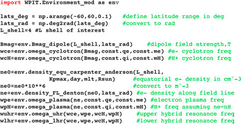
To illustrate how the module is run, the following calling routine calculates the electron and proton gyro-frequency, the local plasma frequency, the upper and lower hybrid frequencies, in the region between −60 and 60° magnetic latitude at L = 4:

2.2 Wave properties module

Module WPIT. WaveProperties_mod includes routines for the characterization of wave properties in the magnetosphere. The routines of the module are presented in Table 2. These include estimations of the Stix parameters, the refractive index, the refractive index based on the Appleton-Hartree approximation, the refractive index of parallel propagating EMIC waves and the dielectric tensor according to cold plasma theory. WPIT includes also routines for the calculation of the above parameters accounting for warm plasma corrections, according to Kulkarni et al. (2015) and Maxworth et al. (2020). Furthermore, this module includes routines for the calculation of the resonance cone angle and the Gendrin angle according to Bortnik et al. (2006), wave electric and magnetic component amplitudes based on the formulations of Bell (1984), Jasna et al. (1992) and Li et al. (2015). WPIT includes a routine to calculate the resonant energy of an electron that interacts with a specific wave and routines to define a wave packet. In the current version of WPIT, a wave packet is defined as the latitudinal profile of the wave amplitude, that can be one sided, two sided or Gaussian in shape with respect to magnetic latitude (see, e.g., Figure 3D). For completeness, WPIT includes also, routines for the calculation of the dispersion relation of different types of waves in plasma, including the R-mode, L-mode, O-mode, X-mode and light, as well as the cut off frequencies of R- and L-mode waves (see, e.g., Swanson (2012)). Detailed description of each routine along with example runs can be found in the WaveProperties_mod_description Jupyter notebook, located in the Module_descriptions folder of the WPIT repository.

TABLE 2

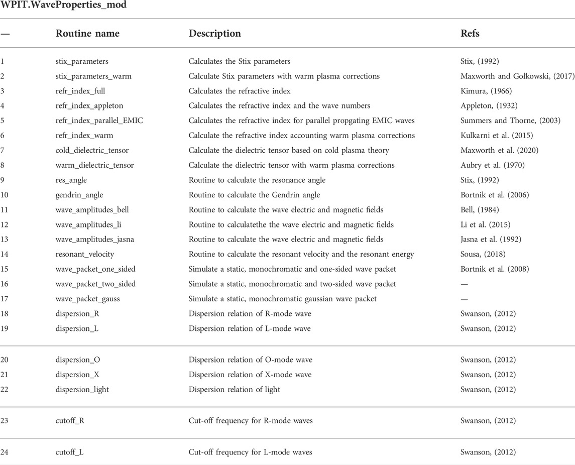
TABLE 2. Wave properties module routines.

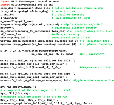
As an illustration of how the module is called, the following routine calculates the Stix parameters, the refractive index and the amplitudes of the electric and magnetic field components of the wave at L = 4 and in the region between −60 and 60° in magnetic latitude:

2.3 Landau damping module

The propagation of a wave within the magnetosphere and the flow of wave power are well-captured by various ray tracing techniques, which trace the path of a monochromatic wave based on geometric optics. Most commonly, ray tracing models are based on cold plasma theory (see, e.g., Kimura, 1966); thus, whereas they provide important parameters of a wave packet, such as its trajectory or the wave normal angle, they assume no attenuation of the wave energy. In the current version of WPIT, Landau damping is applied to a predefined ray path, as obtained from a ray-tracing model (Stanford 3D in the cases presented herein). This approach has been followed by several past studies, such as, e.g., Bell et al. (2002), Sousa (2018), Bortnik et al. (2006), Bortnik et al. (2007), Kulkarni et al. (2008). It is noted that damping or growth of the waves is expected to affect the ray path, and that a more precise approach involves calculating the damping or growth of the wave in a consistent way during the ray tracing calculation; such an approach is followed, for example, in the HOTRAY code (Horne and Thorne, 1993; Horne, 2015; Chen et al., 2009). Introducing results from self-consistent ray tracing simulations, such as HOTRAY, and in particular evaluating the differences in the calculated ray paths and the effects in the resulting wave fields and wave particle interactions compared to the current approach in WPIT that is also commonly used in literature needs to be investigated in further detail.

Module WPIT. LandauDamping_mod enables the estimation of the attenuation of a wave along the ray path according to Landau damping, which refers to the damping of an electromagnetic wave due to its interaction with thermal electrons with velocities that have a component parallel to the ambient geomagnetic field, close to the phase velocity of the wave. The theory behind the calculation of Landau damping is based on the work by Brinca (1972), who expanded upon the work of Kennel (1966).

For the calculation of Landau damping along a ray path the local thermal electron distribution is required, and WPIT enables the selection among four different models, namely:

WPIT. LandauDamp_mod.bell_distribution, which is based on the work by Bell et al. (2002),

WPIT. LandauDamp_mod.bortnik_distribution, which is based on Bortnik et al. (2007),

WPIT. LandauDamp_mod.golden_distribution, which is based on Golden et al. (2010), and

WPIT. LandauDamp_mod.bi_maxwellian_distribution, which is based on Maxworth et al. (2020).

WPIT also enables introducing any user-defined distribution of the form f = f (u_⊥, u_‖).

The local Landau damping of a wave along its propagation path in WPIT is calculated by routine WPIT. LandauDamp_mod.landau_damping. Landau damping calculations in WPIT are based on the work of Sousa (2018) and on the corresponding code found at https://github.com/asousa/damping written in Matlab. For WPIT this code has been transcribed into a Python code, while being further enhanced in terms of usability by enabling the selection of different thermal electron distributions and the integration with outputs from ray tracing simulations.

At the time of writing, the ray paths that are introduced in WPIT are pre-calculated using the Stanford 3D ray tracer based on the code publicly available at https://github.com/asousa/Stanford_Raytracer. WPIT. LandauDamp_mod includes also the sub-module WPIT. LandauDamp_mod.RayUtils which is a collection of routines in relevance with the Ray Tracer output. After a ray tracing simulation is performed with the Stanford 3D Ray Tracer, the ray tracing simulation is exported in . ray format, which includes information such as the wave group velocity, phase velocity, refractive indices, magnetic field as a function of time and position along the ray path. Examples of ray tracing outputs are included in the WPIT github, at https://github.com/stourgai/WPIT/tree/main/Module_descriptions/example_rays. These data files are read in WPIT by routine WPIT. LandauDamp_mod.RayUtils.read_input_ray. Subsequently, using routine WPIT. LandauDamp_mod.RayUtils.append_ray, the required wave properties that are calculated by module WPIT. WaveProperties_mod as described above in Section 2.2, are calculated along the ray path and are appended in a new file that is saved in . csv format. Moreover, routine WPIT. LandauDamp_mod.RayUtils.resonance_along_raypath calculates the velocities and energies of particles that can interact resonantly with the ray-wave for a range of pitch angles. Routine WPIT. LandauDamp_mod.RayUtils.enhancement_factor calculates the magnetospheric cavity enhancement factor as defined in Kulkarni et al. (2006). Finally, routine WPIT. LandauDamp_mod.RayUtils.ray_plots produces plots of the ray path and wave parameters. The routines of the WPIT. LandauDamp_mod module are presented in Table 3.

TABLE 3

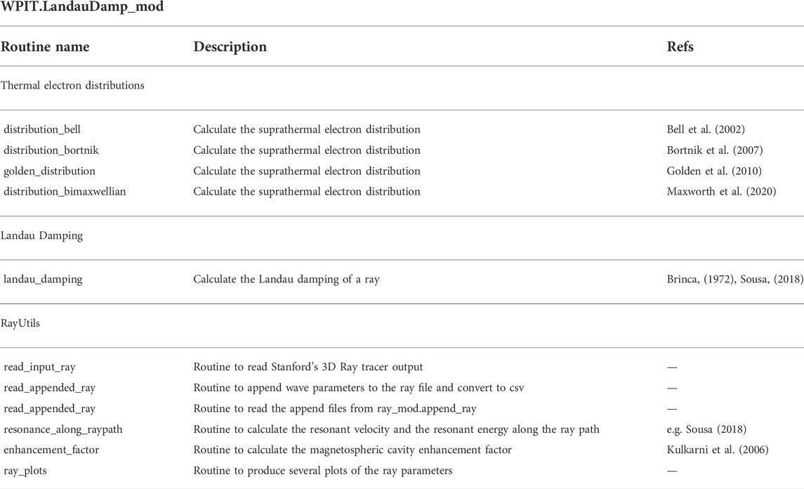
TABLE 3. Landau damping module routines.

Detailed description of each routine along with sample runs can be found in the Module_descriptions folder of the WPIT repository in the corresponding LandauDamp_mod_description Jupyter notebook.

It is noted that WPIT enables incorporating ray path information from ray tracing models other than the Stanford 3D ray tracer, with the proper modification of the routines for importing ray tracer simulation outputs, named WPIT. LandauDamp_mod.RayUtils.read_input_ray.

2.4 Wave—particle interactions module

This module includes routines for estimating the gyro-averaged wave-particle interaction of relativistic particles with a monochromatic wave. The environment and wave properties used in this module are derived from modules WPIT. Enironment_mod and WPIT. WaveProperties_mod, as described above. At the time of writing, WPIT. WPI_mod includes three sub-modules in order to simulate different types of waves and particles: (a) sub-module WPIT. WPI_mod.whistler_electron_mod that is used to simulate the interactions of electrons with whistler mode or magnetosonic waves (either parallel or oblique), (b) sub-module WPIT. WPI_mod.EMIC_ion_mod that is used for the investigation of interactions of ions with EMIC waves (either parallel or oblique) and (c) sub-module WPIT. WPI_mod.parallel_EMIC_mod for the investigation of interactions of either electrons or ions with parallel EMIC waves.

Before introducing in further detail the wave-particle interaction simulations, the formulations of several parameters are discussed, which are required by each of the three types of wave-particle interactions that are tackled in WPIT. These include: dz/dt, which refers to the rate of change of the distance traveled by a particle along the field line; dp_‖/dt, the rate of change of the parallel momentum; dp_⊥/dt, the rate of change of the perpendicular momentum and dη/dt, the rate of change of the wave-particle phase, which in case of WPIT are taken directly from literature. WPIT also includes routines for the calculations of the rate of change of the local pitch angle dα/dt, the rate of change of the equatorial pitch angle dα_eq/dt, the rate of change of the instantaneous particle kinetic energy dE/dt, the rate of change of the relativistic Lorentz factor dγ/dt, and the rate of change of the magnetic latitude, dλ/dt. In the following the methodology for the derivation of each of the above parameters is presented and in the following subsections these are applied specifically for each of the three sub-modules.

The rate of change of the local pitch angle, is based on the derivation:

$\frac{d}{dt}\tan \alpha =\frac{1}{{\cos }^2\alpha }\frac{d\alpha }{dt}$

$\frac{d\alpha }{dt}={\cos }^2\alpha \frac{d}{dt}\tan \alpha ={\cos }^2\alpha \frac{d}{dt}\frac{p_{\perp }}{p_{\Vert }}=\frac{1}{p^2}\left(p_{\Vert }\frac{d{p}_{\perp }}{dt}-p_{\perp }\frac{d{p}_{\Vert }}{dt}\right)(1)$

where α is the local pitch angle, p is the magnitude of the momentum, p_‖ is the component of the momentum parallel to the ambient magnetic field and p_⊥ is the component of the momentum perpendicular to the ambient magnetic field.

The rate of change of the equatorial pitch angle, is derived as:

$\frac{d{\alpha }_{eq}}{dt}=\frac{\tan {\alpha }_{eq}}{\tan \alpha }\left(\frac{d\alpha }{dt}-\frac{p_{\perp }}{2\gamma m_s{\omega }_{ce}}\frac{\partial {\omega }_{cj}}{dz}\right)(2)$

where we made use of the relation between the local and the equatorial pitch angle in a dipole magnetic field. In Eq. 2, α_eq is the local pitch angle, m_s is the particle mass, γ is the Lorentz factor, ω_cj, with j = [e, i], for electrons or ions respectively, is the particle cyclotron frequency and ∂ω_cj/∂z is the gradient of the cyclotron frequency along the field line.

The kinetic energy and the Lorentz factor γ are derived based on the following equations:

$\frac{d{E}_k}{dt}=\frac{1}{\gamma m_s}\left(p_{\Vert }\frac{d{p}_{\Vert }}{dt}+p_{\perp }\frac{d{p}_{\perp }}{dt}\right)(3)$

$\frac{d\gamma }{dt}=\frac{d}{dt}\frac{E_k}{m_s{c}^2}=\frac{1}{\gamma m_s^2{c}^2}\left(p_{\Vert }\frac{d{p}_{\Vert }}{dt}+p_{\perp }\frac{d{p}_{\perp }}{dt}\right)(4)$

where E_k is the particle’s kinetic energy, c is the speed of light and the remaining terms as defined above.

Finally, for the rate of change of the particle’s magnetic latitude, we use the following equation, that relates the distance along a field with the latitude for a dipole field:

$dz=L{R}_e{\left(1+3{\sin }^2\lambda \right)}^{1/2}\cos \lambda d\lambda (5)$

thus

$\frac{d\lambda }{dt}=\frac{d\lambda }{dz}\frac{dz}{dt}=\frac{1}{L{R}_e{\left(1+3{\sin }^2\lambda \right)}^{1/2}\cos \lambda }\frac{p_{\Vert }}{\gamma m_s}(6)$

where we used:

$\frac{dz}{dt}=\frac{p_{\Vert }}{\gamma m_s}(7)$

where λ is the latitude, z is the distance along the field line, L is the L shell, R_e is the Earth’s radius, m_s is the particle’s mass and all the other parameters as defined previously. Equations 6 and 7 will be used in the following Sections 2.4.1, Section 2.4.2 and Section 2.4.3.

For the investigation and quantification of nonlinear effects during wave-particle interactions, we derive the relevant equations for each module based on the reasoning of Su et al. (2014).

We start by calculating the second derivative of the wave-particle phase, and we transform the resulting equation in the form:

$\frac{d\nu }{dt}={\omega }_t^{2}sign\left(\theta \right)\sin \eta +H={\omega }_t^2\left[sign\left(\theta \right)\sin \eta +S\right](8)$

with

$S=\frac{H}{{\omega }_t^2}(9)$

and

$\nu =\frac{d\eta }{dt}(10)$

ω_t is the trapping frequency, and S is a ratio that defines the relative importance of the wave induced motion to the adiabatic motion. When |S| > 1 the adiabatic motion dominates, while when |S| < 1 the wave induced motion prevails (Su et al., 2014).

The routines of each sub-module are presented in the following sub-sections.

2.4.1 Whistler mode—electron interactions module

The routines of this module can be used for the investigation of the interactions of electrons with whistler or magnetosonic waves. The equations for the calculation of dp_‖/dt, dp_⊥/dt and dη/dt are derived from Bortnik et al. (2015).

The evolution of the component of the electron momentum parallel to the magnetic field, p_‖, is calculated as:

$\frac{d{p}_{\Vert }}{dt}={\omega }_{\tau m}^2{m}_e{k}_z^{-1}\sin \eta -\frac{1}{\gamma m_e}\frac{p_{\perp }^2}{2{\omega }_H}\frac{\partial {\omega }_{ce}}{\partial z}(11)$

while the corresponding term for the perpendicular component, p_⊥, is calculated as:

$\begin{array}{ll}\hfill \frac{d{p}_{\perp }}{dt}& =-{\left(-1\right)}^{m-1}\left[{\omega }_1\left(\frac{p_z}{\gamma }+m_e{R}_1\right)J_{m-1}\left(\beta \right)\right.\hfill \\ \hfill & -\left.{\omega }_2\left(\frac{p_z}{\gamma }-m_e{R}_2\right)J_{m+1}\left(\beta \right)\right]\sin \eta +\frac{1}{\gamma m_e}\frac{p_{\perp }{p}_z}{2{\omega }_H}\frac{\partial {\omega }_{ce}}{\partial z}\hfill \end{array}(12)$

and the evolution of electron-wave phase η is calculated as:

$\frac{d\eta }{dt}=\frac{m{\omega }_{ce}}{\gamma }-\omega -k_z\frac{p_z}{\gamma m_e}(13)$

where

$\begin{array}{cc}\hfill \beta & =\frac{k_x{p}_{\perp }}{m_e\gamma {\omega }_{ce}},k_z=k\cos \psi =\left(\mu \omega /c\right)\cos \psi ,k_x=k\sin \theta \hfill \\ \hfill {\omega }_{\tau m}^2& ={\left(-1\right)}^{m-1}{\omega }_{\tau 0}^2\left[J_{m-1}\left(\beta \right)-{\alpha }_1{J}_{m+1}\left(\beta \right)+\gamma {\alpha }_2{J}_m\left(\beta \right)\right]\hfill \\ \hfill {\omega }_{\tau 0}^2& =\frac{{\omega }_1{k}_z{p}_{\perp }}{\gamma m_e},{\omega }_1=\frac{e}{2m_e}\left(B_x^w+B_y^w\right),{\omega }_2=\frac{e}{2m_e}\left(B_x^w-B_y^w\right),\hfill \\ \hfill {\alpha }_1& =\frac{{\omega }_2}{{\omega }_1}\hfill \\ \hfill {\alpha }_2& =\frac{e{E}_z^w}{{\omega }_1{p}_{\perp }},R_1=\frac{E_x^w+E_y^w}{B_x^w+B_y^w},R_2=\frac{E_x^w-E_y^w}{B_x^w-B_y^w}\hfill \end{array}(14)$

where μ is the refractive index, ψ is the wave normal angle, J_i are Bessel functions of the first kind, of order i and argument β, k_x and k_z are the x and z components of the wave number k, ω_ce is the electron cyclotron frequency and $B_j^w$ and $E_j^w$, with j = [x, y, z], are the magnetic and electric field components of the wave.

By applying Eqs 1–4, we derive the set of auxiliary equations for the sub-module related to whistler-electron interactions:

$\begin{array}{cc}\hfill \frac{d\alpha }{dt}& =-\frac{1}{p^2}\left\{{\left(-1\right)}^{m-1}\left[{\omega }_1\left(\frac{p_{\Vert }}{\gamma }+m_e{R}_1\right)J_{m-1}\left(\beta \right)\right.\right.\hfill \\ \hfill & -\left.{\omega }_2\left(\frac{p_{\Vert }}{\gamma }-m_e{R}_2\right)J_{m+1}\left(\beta \right)\right]p_{\Vert }\hfill \\ \hfill & +\left.{\omega }_{\tau m}^2{m}_e{k}_{\Vert }^{-1}{p}_{\perp }\right\}\sin \eta +\frac{1}{m_e\gamma }\frac{p_{\Vert }{p}^2}{2{\omega }_H}\frac{\partial {\omega }_{ce}}{\partial z}\hfill \end{array}(15)$

$\begin{array}{cc}\hfill \frac{d{\alpha }_{eq}}{dt}& =-\frac{1}{p^2}\frac{\tan {\alpha }_{eq}}{\tan \alpha }\left\{{\left(-1\right)}^{m-1}\left[{\omega }_1\left(\frac{p_{\Vert }}{\gamma }+m_e{R}_1\right)J_{m-1}\left(\beta \right)\right.\right.\hfill \\ \hfill & -\left.{\omega }_2\left(\frac{p_{\Vert }}{\gamma }-m_e{R}_2\right)J_{m+1}\left(\beta \right)\right]p_{\Vert }\hfill \\ \hfill & +\left.{\omega }_{\tau m}^2{m}_e{k}_z^{-1}{p}_{\perp }\right\}\sin \eta \hfill \end{array}(16)$

$\begin{array}{ll}\hfill \frac{d{E}_k}{dt}& ={\left(-1\right)}^{m-1}\frac{e}{\gamma m_e}\left[E_z^w{p}_{\Vert }{J}_m\left(\beta \right)-p_{\perp }{E}_L{J}_{m+1}\left(\beta \right)\right.\hfill \\ \hfill & -\left.p_{\perp }{E}_R{J}_{m-1}\left(\beta \right)\right]\sin \eta \hfill \end{array}(17)$

$\begin{array}{ll}\hfill \frac{d\gamma }{dt}& ={\left(-1\right)}^{m-1}\frac{e}{\gamma m_e^2{c}^2}\left[E_z^w{p}_{\Vert }{J}_m\left(\beta \right)\right.\hfill \\ \hfill & -\left.p_{\perp }{E}_L{J}_{m+1}\left(\beta \right)-p_{\perp }{E}_R{J}_{m-1}\left(\beta \right)\right]\sin \eta \hfill \end{array}(18)$

For the investigation of nonlinear effects we derive eight for the case of whistler-electron interactions. The resulting equations are:

$H=\frac{m}{\gamma }\frac{d{\omega }_{ce}}{dt}+\frac{p_{\Vert }}{\gamma m_e}\frac{d{k}_{\Vert }}{dt}-\frac{d{\omega }_{ce}}{dt}-\frac{k_{\Vert }{p}_{\perp }^2}{2{\gamma }^2{m}_e^2{\omega }_{ce}}\frac{\partial {\omega }_{ce}}{\partial z}(19)$

$\theta =C_0{J}_m\left(\beta \right)+C_{+1}{J}_{m+1}\left(\beta \right)+C_{-1}{J}_{m-1}\left(\beta \right)(20)$

$C_0=-{\left(-1\right)}^{m-1}\left[\frac{q_e{p}_{\Vert }}{{\gamma }^3{m}_e^2{c}^2}\left(m{\omega }_{ce}-\frac{k_{\Vert }{p}_{\Vert }}{m_e}\right)+\frac{k_{\Vert }{q}_e}{\gamma m_e}\right]E_z^w(21)$

$C_{+1}={\left(-1\right)}^{m-1}\left[\frac{q_e{p}_{\perp }{E}_L}{{\gamma }^3{m}_e^2{c}^2}\left(m{\omega }_{ce}-\frac{k_{\Vert }{p}_{\Vert }}{m_e}\right)+\frac{p_{\perp }{k}_{\Vert }{\omega }_2}{m{\gamma }^2}\right](22)$

$C_{-1}={\left(-1\right)}^{m-1}\left[\frac{q_e{p}_{\perp }{E}_R}{{\gamma }^3{m}_e^2{c}^2}\left(m{\omega }_{ce}-\frac{k_{\Vert }{p}_{\Vert }}{m_e}\right)-\frac{p_{\perp }{k}_{\Vert }{\omega }_1}{m{\gamma }^2}\right](23)$

The corresponding routines that incorporate the above equations are presented in Table 4.

TABLE 4

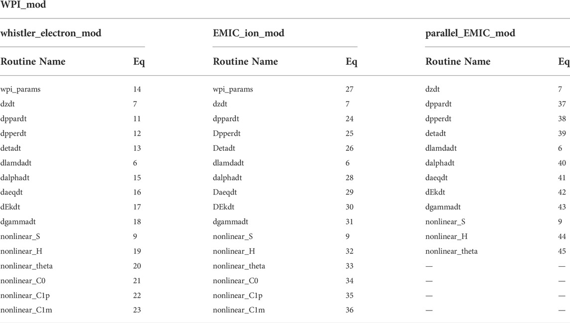
TABLE 4. WPI modlule routines.

2.4.2 EMIC wave—ion interactions module

The routines of this module can be used for the investigation of the interactions of ions with EMIC waves. The equations for the calculation of dp_‖/dt, dp_⊥/dt and dη/dt are derived from (Su et al., 2014).

The evolution of the component of the electron momentum that is parallel to the magnetic field, p_‖, is calculated as:

$\begin{array}{ll}\hfill \frac{d{p}_{\Vert }}{dt}& ={\left(-1\right)}^{l+1}\left[q{E}_w^z{J}_l\left(\beta \right)-{\omega }_R{p}_{\perp }{J}_{l+1}\left(\beta \right)+{\omega }_L{p}_{\perp }{J}_{l-1}\left(\beta \right)\right]\hfill \\ \hfill & \times \sin \eta -\frac{p_{\perp }^2}{2\gamma m{\omega }_{ci}}\frac{\partial {\omega }_{ci}}{\partial z}\hfill \end{array}(24)$

while for the corresponding term for the perpendicular component, p_⊥, is calculated as:

$\begin{array}{ll}\hfill \frac{d{p}_{\perp }}{dt}& ={\left(-1\right)}^{l+1}\left[\left(p_{\Vert }-p_w^R\right){\omega }_R{J}_{l+1}\left(\beta \right)\right.\hfill \\ \hfill & -\left.\left(p_{\Vert }-p_w^L\right){\omega }_L{J}_{l-1}\left(\beta \right)\right]\sin \eta +\frac{p_{\perp }{p}_{\Vert }}{2\gamma m{\omega }_{ci}}\frac{\partial {\omega }_{ci}}{\partial z}\hfill \end{array}(25)$

The evolution of the ion-wave phase η is calculated as:

$\frac{d\eta }{dt}=\frac{l{\omega }_{ci}}{\gamma }+\frac{k_{\Vert }{p}_{\Vert }}{\gamma m}-\omega (26)$

where

$\begin{array}{cc}\hfill \beta & =-\frac{k_{\perp }{p}_{\perp }}{q{B}_D},p_w^R=\gamma m\frac{E_w^R}{B_w^R},p_w^L=\gamma m\frac{E_w^L}{B_w^L},B_w^R=\frac{B_w^x+B_w^y}{2}\hfill \\ \hfill B_w^L& =\frac{B_w^x-B_w^y}{2},E_w^R=\frac{E_w^x+E_w^y}{2},E_w^L=\frac{E_w^x-E_w^y}{2},{\omega }_R=\frac{q{B}_w^R}{\gamma m},\hfill \\ \hfill {\omega }_L& =\frac{q{B}_w^L}{\gamma m}\hfill \end{array}(27)$

where B_D is dipole field strength.

By applying Eqs 1–4 for the case of EMIC waves, we get:

$\begin{array}{cc}\hfill \frac{d\alpha }{dt}& ={\left(-1\right)}^{l+1}\frac{\sin \eta }{p^2}\left[q{E}_w^z{p}_{\Vert }{J}_l\left(\beta \right)-{\omega }_R{p}_w^R{p}_{\perp }{J}_{l+1}\left(\beta \right)\right.\hfill \\ \hfill & +\left.{\omega }_L{p}_w^L{p}_{\perp }{J}_{l+1}\left(\beta \right)\right]\hfill \end{array}(28)$

$\begin{array}{cc}\hfill \frac{d{\alpha }_{eq}}{dt}& ={\left(-1\right)}^{l+1}\frac{p_{\Vert }}{p_{\perp }}\frac{\tan {\alpha }_{eq}\sin \eta }{p^2}\left[-q{E}_w^z{p}_{\perp }{J}_l\left(\beta \right)\right.\hfill \\ \hfill & +\left.{\omega }_R\left(p^2-p_w^R{p}_{\Vert }\right)J_{l+1}\left(\beta \right)-{\omega }_L\left(p^2+p_w^L{p}_{\Vert }\right)J_{l-1}\left(\beta \right)\right]\hfill \end{array}(29)$

$\begin{array}{ll}\hfill \frac{d{E}_k}{dt}& ={\left(-1\right)}^{l+1}\frac{q}{m\gamma }\left[E_w^z{p}_{\Vert }{J}_l\left(\beta \right)-E_w^R{p}_{\perp }{J}_{l+1}\left(\beta \right)\right.\hfill \\ \hfill & -\left.E_w^L{p}_{\perp }{J}_{l-1}\left(\beta \right)\right]\sin \eta \hfill \end{array}(30)$

$\begin{array}{ll}\hfill \frac{d\gamma }{dt}& ={\left(-1\right)}^{l+1}\frac{q}{\gamma m^2{c}^2}\left[E_w^z{p}_{\Vert }{J}_l\left(\beta \right)\right.\hfill \\ \hfill & -\left.E_w^R{p}_{\perp }{J}_{l+1}\left(\beta \right)-E_w^L{p}_{\perp }{J}_{l-1}\left(\beta \right)\right]\sin \eta \hfill \end{array}(31)$

For the investigation of nonlinear effects related to the interaction of EMIC waves with ions, WPIT uses the approximation and equations described in (Su et al., 2014):

$H=\frac{l}{\gamma }\frac{d{\omega }_{ci}}{dt}+\frac{p_{\Vert }}{\gamma m}\frac{d{k}_{\Vert }}{dt}-\frac{d\omega }{dt}-\frac{k_{\Vert }{p}_{\perp }^2}{2{\gamma }^2{m}^2\mathrm{\Omega }}\frac{\partial {\omega }_{ci}}{\partial z}(32)$

$\theta =C_0{J}_l\left(\beta \right)+C_{+1}{J}_{l+1}\left(\beta \right)+C_{-1}{J}_{l-1}\left(\beta \right)(33)$

$C_0={\left(-1\right)}^{l+1}\left[\frac{q{k}_{\Vert }}{\gamma m}-\frac{q{p}_{\Vert }}{{\gamma }^3{m}^2{c}^2}\left(l{\omega }_{ci}+\frac{k_{\Vert }{p}_{\Vert }}{m}\right)\right]E_w^z(34)$

$C_{+1}={\left(-1\right)}^{l+1}\left[-\frac{{\omega }_R{k}_{\Vert }}{\gamma m}+\frac{q{E}_w^R}{{\gamma }^3{m}^2{x}^2}\left(l{\omega }_{ci}+\frac{k_{\Vert }{p}_{\Vert }}{m}\right)\right]p_{\perp }(35)$

$C_{-1}={\left(-1\right)}^{l+1}\left[\frac{{\omega }_L{k}_{\Vert }}{\gamma m}+\frac{q{E}_w^L}{{\gamma }^3{m}^2{x}^2}\left(l{\omega }_{ci}+\frac{k_{\Vert }{p}_{\Vert }}{m}\right)\right]p_{\perp }(36)$

The corresponding routines that incorporate the above equations are presented in Table 4.

2.4.3 Parallel EMIC wave—electron & ion interactions module

The routines of this module can be used for the investigation of the interactions of either electrons or ions with parallel propagating EMIC waves. The equations for the calculation of dp_‖/dt, dp_⊥/dt and dη/dt are derived from (Su et al., 2013):

$\frac{d{p}_{\Vert }}{dt}=\frac{e{B}_w}{\gamma m}{p}_{\perp }\sin \eta -\frac{p_{\perp }^2}{2\gamma m{\omega }_{cj}}\frac{\partial {\omega }_{cj}}{\partial z}(37)$

$\frac{d{p}_{\perp }}{dt}=e{B}_w\left(\frac{\omega }{k}-\frac{p_{\Vert }}{\gamma m}\right)\sin \eta +\frac{p_{\perp }{p}_{\Vert }}{2\gamma m{\omega }_{cj}}\frac{\partial {\omega }_{cj}}{\partial z}(38)$

$\frac{d\eta }{dt}=\frac{e{B}_w}{p_{\perp }}\left(\frac{\omega }{k}-\frac{p_{\Vert }}{\gamma m}\right)\cos \eta +\left(\frac{k{p}_{\Vert }}{\gamma m}-\omega -\frac{|{\omega }_{cj}|}{\gamma }\right)(39)$

By applying Eqs 1–4 for the parallel EMIC case, we get:

$\begin{array}{c}\hfill \frac{d\alpha }{dt}=\frac{e{B}_w}{p^2}\left[\left(\frac{\omega }{k}-\frac{p}{\gamma m}\right)p_{\Vert }-\frac{p_{\perp }^2}{\gamma m}\right]\sin \eta +\frac{p_{\perp }}{2\gamma m{\omega }_c}\frac{\partial {\omega }_{cj}}{\partial z}\end{array}(40)$

$\begin{array}{c}\hfill \frac{d{\alpha }_{eq}}{dt}=\frac{e{B}_w}{p^2}\frac{\tan {\alpha }_{eq}}{\tan \alpha }\left[\left(\frac{\omega }{k}-\frac{p_{\Vert }}{\gamma m}\right)p_{\Vert }-\frac{p_{\perp }^2}{\gamma m}\right]\sin \eta \end{array}(41)$

$\frac{d{E}_k}{dt}=e{B}_w\frac{\omega }{k}\frac{p_{\perp }}{\gamma m}\sin \eta (42)$

$\frac{d\gamma }{dt}=e{B}_w\frac{\omega }{k}\frac{p_{\perp }}{\gamma m^2{c}^2}\sin \eta (43)$

For the investigation of nonlinear effects we derive eight for the case of parallel EMIC waves. The resulting equations are:

$H=-\frac{1}{\gamma }\frac{d{\omega }_{cj}}{dt}+\frac{p_{\Vert }}{\gamma m}\frac{d{k}_{\Vert }}{dt}-\frac{d\omega }{dt}-\frac{k_{\Vert }{p}_{\perp }^2}{2{\gamma }^2{m}^2{\omega }_{cj}}\frac{\partial {\omega }_{cj}}{\partial z}(44)$

$\theta =e{B}_w{p}_{\perp }\left[\frac{k}{{\gamma }^2{m}^2}+\left({\omega }_c-\frac{k_{\Vert }{p}_{\Vert }}{m}\frac{\omega }{k{\gamma }^{3}m{c}^2}\right)\right](45)$

The corresponding routines that incorporate the above equations are presented in Table 4.

2.5 Integration

Based on the equations described above, wave-particle interaction parameters are estimated along a particle’s trajectory via the integration of the corresponding differential equations. For the simulations presented herein, we used a 4^th order Runge-Kutta integrator, but a user of WPIT could use any convenient integrator to integrate the differential equations of the particle. The set-up of the integrator for each simulation can be found in the corresponding Jupyter notebooks in WPIT_Results and WPIT_tests folders of WPIT repository.

2.6 WPIT requirements

Apart from the modules described above, WPIT requires the installation of some open source Python packages. These are the matplotilb, the numpy, the pandas, the scipy, the spacepy and the notebook packages. Matplotlib is a visualization library in Python and it is used for producing all the output figures of the WPIT repository. Numpy is a package for scientific computing in Python. In WPIT it is called in all of the routines for performing mathematical calculations. Pandas is a tool for data analysis. It is used for reading and writing data files in WPIT. Scipy is a set of algorithms for scientiffic computing. WPIT uses the scipy. special module for the calculation of Bessel functions. Finally, the installation of the notebook package, enables the use of Jupyter Notebooks. The version of each package used in WPIT testing and an installation file is included in the WPIT repository (https://github.com/stourgai/WPIT/blob/main/requirements.txt).

2.7 Importing WPIT modules

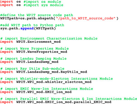
It is noted that in its current version, WPIT does not include a setup file. Thus, the user must add the WPIT source code path to the Python path. This is done as follows: the built-in Python modules os and sys should be imported first. The os module implements functions on pathnames, while the sys module contains parameters specific to the system. The os. path.abspath() function is first used to define the path of the WPIT folder which contains the source code of the package; subsequently the sys. path.append() function is used to add the WPIT source code path to the Python path. Then the WPIT modules can be imported to the code. In the following, we present a code snippet which illustrates this procedure:

2.8 Methodology verification

For the verification of the WPIT code and as a demonstration of its capabilities, the results from a number of key past studies related to wave-particle interactions are reproduced using WPIT. These include results: Bortnik et al. (2008), Albert and Bortnik (2009), Su et al. (2012) and Su et al. (2014). The corresponding parameterizations of WPIT that reproduce the results of the above studies are formatted as Jupyter notebooks and are included in the project’s folder WPIT_tests located at https://github.com/stourgai/WPIT/tree/main/WPIT_tests. It is noted that these Jupyter notebooks confirming past results can also be used as tutorials for the use of the WPIT routines. Reproductions of results of these publications are presented in Supplementary Figures S1-S12 as follows: results by Bortnik et al. (2008) are included as Supplementary Figures S1-S3; results by Albert and Bortnik (2009) are included as Supplementary Figures S4-S6; results by Su et al. (2012) are included as Supplementary Figures S7, S8; and results by Su et al. (2014) are included as Supplementary Figures S9-S12.

3 Results

In the following, and in order to present the capabilities of WPIT, simulation outputs are presented for each of the four WPIT modules. As a case study, we expand upon the simulations by Bortnik et al. (2008) through a parametric study that explores the impact of each parameter in the onset of nonlinearity in whistler-electron interactions. More specifically, the dependence of the appearance of nonlinear effects on wave field amplitude, equatorial pitch angle, wave normal angle, electron energy, electron density, wave frequency and ion composition are explored.

We first define a baseline simulation that follows the simulation parameters introduced in Bortnik et al. (2008), with some variations discussed in the following:

Bortnik et al. (2008) studied the interactions of electrons with whistler-mode waves at L = 5, in a dipole geomagnetic field and in a multi-component plasma with equatorial electron density n_e,eq = 10 cm⁻³. They simulated a total of 24 electrons with equatorial pitch angle α_eq = 70°, energy E = 168.3 keV and equally spaced in wave-particle phase, in the range 0–360°, thus they had a resolution of 5° in initial wave-particle phase. The electrons started at an initial latitude of λ = −9° and were followed until they reached the magnetic equator. The wave packet used was static, monochromatic and one-sided, with a frequency of 2 kHz and wave normal angle of ψ = 0°. Two wave amplitudes of 1pT and 1nT were investigated.

For our baseline simulation, we retain the latitudinal range, the equatorial electron density, the electron energy and the wave packet morphology, frequency and wave normal angle of Bortnik et al. (2008). We simulate the variation of the electron density along the magnetic field line using the (Denton et al., 2002) model. The ion composition is taken as n_H = 0.77n_e for H⁺ ions, n_He = 0.20n_e for He⁺ ions and n_O = 0.03n_e for O⁺ ions (Jordanova et al., 2008). As was derived from our simulations (not shown here, but the results are available at WPIT_results folder of WPIT repository), there is a need for higher resolution in the initial wave-particle phase, as there are nonlinear effects that can be missed if the wave-particle phase resolution is not high enough. From our simulations, during the evaluation phase of WPIT, we found that a minimum resolution of 3° is required in order to fully resolve non linear interactions. Hence, for our simulations we explore the behaviour of 120 electrons equally spaced in initial wave-particle angle η₀ in the range 0–360° thus achieving the wave-particle phase resolution threshold. The initial equatorial pitch angle is chosen at 68°. Finally, the amplitude of the y-component of the wave magnetic field is chosen at 65pT in the baseline simulation.

We start by presenting outputs of the Environment_mod and the WaveProperties_mod modules for the baseline simulation, in Section 3.1 and Section 3.2 respectively. We then present a sample run from the LandauDamp_mod module corresponding to the above conditions in Section 3.3. Finally, we proceed to exploring the onset of nonlinearity of wave-particle interactions by varying each parameter of the baseline simulation separately, in Section 3.4.

The corresponding Jupyter Notebooks for each simulation can be found in https://github.com/stourgai/WPIT/tree/main/WPIT_results.

3.1 Environment characterization module results

For the calculation of required local environment parameters we use the WPIT/Environment_mod module. In Figure 2 we present environmental parameters of the simulation as a function of the magnetic latitude. In Figure 2A, we present the magnetic dipole field strength as calculated by the routine WPIT. Environment_mod.Bmag_dipole, in Figure 2B, the electron and ion densities calculated by WPIT. Environment_mod.density_FL_denton with an equatorial electron density of 10cm⁻³, in Figure 2C relevant frequencies (i.e. wave, cyclotron, plasma, upper hybrid resonance and lower hybrid resonance frequencies). In the baseline simulation the wave frequency lies above the lower hybrid resonance frequency but well below the electron cyclotron frequency. In Figure 2D, we present the equatorial pitch angles corresponding to the maximum latitude that a particle can reach in a dipole magnetic field. Each graph spans magnetic latitudes in the range −45 to 45°, with the inset figures zooming-in in the region of interest for our simulations.

FIGURE 2

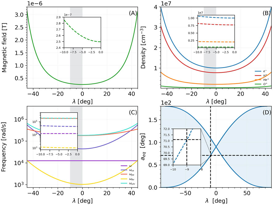
FIGURE 2. Outputs of WPIT. Environment_mod. (A): Background dipole magnetic field. (B): Electron and ion densities. (C): Frequencies. (D): Equatorial pitch angle mapping.

The code for the calculations can be found in WPIT_results/Environment_Results notebook.

3.2 Wave properties module results

With respect to the wave field of the simulation we simulate a static monochromatic parallel propagating whistler-mode wave with a frequency of 2 kHz (Bortnik et al., 2008). With the environmental parameters defined, we calculate the required wave properties for the definition of the whistler-mode wave, which include the Stix parameters, the refractive index, the wave number and the resonance cone angle, as described in Section 2.2. As examples, in Figure 3A we present the Stix parameters along the magnetic latitude calculated by WPIT. WaveProperties_mod.stix_parameters. In Figure 3B we plot the refractive index surface of a 2 kHz wave at the equator, at L = 5. We calculate the surface based on both cold plasma theory and also by assigning finite temperatures to the electron and ion populations. The code for calculating the refractive index surface can be found in the relevant Jupyter notebook [WPIT_results/Environment_And_Wave_Results]. As also mentioned in Kulkarni et al. (2015), the inclusion of finite temperatures in electron and ion populations closes the refractive index surface, which remains open based on the cold plasma theory. Here, as examples of this behaviour, we calculated the refractive index surface for 1 eV electrons and also for 4 eV electrons 4 eV ions. In Figure 3C the resonance cone angle is plotted (WPIT.WaveProperties_mod.refr_index_full) and in Figure 3D the calculated electric and magnetic components of a 2 kHz parallel wave with $B_y^w=100pT$ are shown. Here we have used the WPIT. WaveProperties_mod.wave_packet_one_sided for the definition of the wave packet along with WPIT. WaveProperties_mod.wave_amplitudes_bell for the calculation of the wave field components, to define a one-sided wave packet similarly to Bortnik et al. (2008). As the wave normal angle for this case is considered zero (i.e. parallel propagation) the x- and y-components of the wave electric and magnetic field are the same while the z-components are zero. This condition will change for oblique waves. Also, the electric field decreases as the wave reaches the equator. This behaviour is explained from the dispersion relation of the wave, which determines that the ratio of the electric wave field to the magnetic wave field decreases as the geomagnetic field strength decreases, hence for our case where the y-component of the wave magnetic field is fixed (Bell, 1984) the electric field component has its minimum at the equator.

FIGURE 3

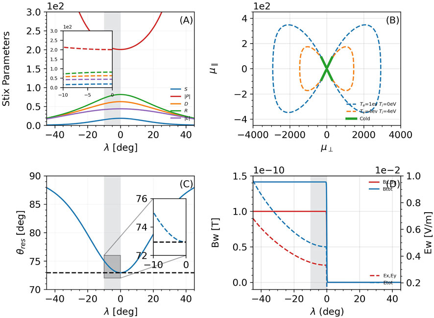
FIGURE 3. Outputs of WPIT. WaveProperties_mod. (A): Stix parameters. (B): Refractive index surface. (C): Resonance cone angle. (D): Wave electric and magnetic fields for a wave with B_yw =100pT.

3.3 Landau damping module results

We performed ray tracing simulations with the Stanford 3D Raytracer, for a ray of f = 2 kHz, injected at the magnetic equator (λ = 0) of L = 5 and with initial wave normal angle ψ = 180°, i.e. anti-parallel to the ambient magnetic field. The raytracer output can be found in Module_descriptions/example_rays folder of WPIT repository. Figure 4 presents example outputs of LandauDamp_mod module. In Figure 4A we present different thermal electron distributions calculated with WPIT. LandauDamp_mod.distribution_bell (Bell et al., 2002) and WPIT. LandauDamp_mod.distribution_bortnik (Bortnik et al., 2007) routines. Bortnik et al. (2006) used a distribution of suprathermal electrons of $f_0=10f_0^{\mathit{Bell}}$, where $f_0^{\mathit{Bell}}$ is the Bell et al. (2002) distribution. This scaling was applied in order to account for fluxes outside of the plasmasphere as the Bell distribution was derived from measurements inside the plasmapause. Furthermore (Bortnik et al., 2007), investigated the effects of different scaling factors of the distribution on Landau damping. Following a similar analysis, we calculated Landau damping for three cases: (i) the original Bell distribution (“scale = 1”), (ii) a distribution multiplied by a factor of 5 (termed as “scale = 5” herein) and (iii) a distribution multiplied by a factor of ten (termed “scale = 10”). For each of these distributions we calculate the Landau damping with WPIT. LandauDamp_mod.landau_damping routine and the results are presented in Figure 4B. For the original Bell distribution, the ray attenuates at around 7 s. Scaling up the distribution 5 and 10 times leads to an attenuation time of 5 and 2.5 s respectively. While for the Bortnik distribution, the ray survives for only about 1 s. Thus, it becomes obvious that the choice of the thermal distribution is a crucial part of Landau damping calculations. Following on, in Figure 4C we present the resonant energy of electrons of pitch angles, in the range 0–90°, with the wave along the ray path [WPIT.LandauDamp_mod.resonance_along_raypath]. The colorscale is in log (E_res) with E_res the resonant energy in keV. It is mentioned that in this plot we calculate the resonant energy along the ray path without taking account the attenuation, thus the time axis ranges from 0 up to 30s, although after 7 s the wave would be damped. Finally, in Figure 4D we present the ray path with color coded the Landau damping [WPIT.LandauDamp_mod.RayUtils_mod.ray_plots] for the Bell distribution case. The yellow dot indicates the injection point of the ray and the black arrow indicates the initial wave normal angle.

FIGURE 4

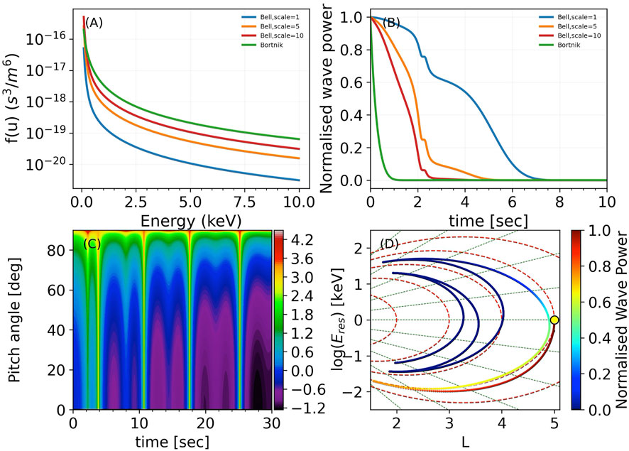
FIGURE 4. Outputs of WPIT. LandauDamp_mod. (A): Thermal electron distributions. (B): Landau damping calculations for each distribution. (C): Electron resonant energy along the ray path for a range of pitch angles. (D): Ray path with color coded Landau damping.

3.4 Wave—particle interactions module results

Firstly, we explore the dependence of the onset of nonlinearity on the amplitude of the y-component of the wave magnetic field, as wave amplitude is the primary parameter in controlling the nonlinear behaviour of the particles, as also discussed in Bell (1986). There are two kinds of nonlinear effects that can arise: phase trapping and phase bunching. During phase trapping, particles follows closed trajectories in ν − η plane, around the center of a resonance island. In this case particles stay in resonance with the wave for a significant amount of time, which leads to large changes in pitch angle and energy. On the other hand, during phase bunching, particles follow open trajectories that enclose the resonance island. As the particles move in ν − η plane, they gradually approach the resonance island. This leads to some particles showing clustered trajectories (termed “bunching” of the trajectories); subsequently the particles cross to the other side of the island and then diverge away from it (see, e.g., Albert et al., 2012). In η − λ plane, the trajectories of phase trapped particles experience several oscillations, which are confined to a limited range of wave-particle phases. On the other hand, trajectories of phase bunched particles are clustered, and span the entire range (0–360°) in phase (see, e.g., Su et al., 2014). As mentioned above, we use Bell (1984) for the calculation of the wave components, which requires the amplitude of the y-component of the wave magnetic field to be defined first in order for the rest of the magnetic and electric field components to be determined. Thus in our simulations we consider a constant $B_y^w$ component along the electron path, modulated only by the wave packet definition, as described above in Section 3.2 and shown in Figure 3D). In Figure 5 we present the trajectories of the 120 electrons for $B_y^w$ = 10pT, 35pT, 65pT and 100pT. The line colors correspond to the initial wave-particle phase (η₀) of the electrons, from 0 to 360°. In the first row we plot the evolution of the equatorial pitch angle (Δα_eq) along the magnetic latitude (λ). In the second row we plot the net change of the equatorial pitch angle as a function of the electrons’ η₀. In the third row we plot the time derivative of η, dη/dt, along the magnetic latitude. In the last row we plot the first derivative of η, ν, normalised to the trapping frequency (ω_t), as a function of η.

FIGURE 5

FIGURE 5. Evolution of α_eq along λ (A,E,I,M), distribution of Δα_eq with respect to the initial wave-particle phase η₀ (B,F,J,N), derivative of wave-particle phase η along λ (C,G,K,O) and electron trajectories in the ν-η plane (D,H,L,P) for different values of the wave magnetic field y-component.

In all cases, the electrons experience resonance with the waves, which can be seen from the plots on the third row, as the resonance condition is expressed as:

$\frac{d\eta }{dt}=0(46)$

The resonance location for all four amplitudes is at λ ≈ − 6.2°. For the 10pT case the interactions are rather linear with small pitch angle scattering and the change in pitch angle follows an almost sinusoidal dependence on η₀, with |Δα_eq|_max ≈ 0.5°. For all amplitudes from 35pT and higher phase trapping effects are observed. For the 35pT case, five out of the 120 electrons, with η₀ in the range 160–173°, experience phase trapping, following closed trajectories in the ν − η plane, and their dη/dt oscillates around 0 throughout the simulation. As the amplitude increases to 65pT, the number of phase trapped electrons increases to 16, binned in four regions of η₀, approximately at 0–10, 156–167, 270–290 and 358–360°, whereas the untrapped electrons are almost symmetrically scattered to lower and higher equatorial pitch angles. The amplitude of the oscillation of their dη/dt also becomes higher. Finally, at 100pT, the trajectories are similar, with 8 phase trapped electrons, but in this case the majority of the untrapped electrons are scattered to lower pitch angles. Three ranges of η₀ experience phase trapping in this case, approximately at 51–55, 158–168 and 238–245°. It is noted, that as the wave field becomes higher, dη/dt oscillates around 0 with higher amplitude, which in turn leads to oscillations of the pitch angles of the trapped electrons around a mean value. Based also on simulations of other wave amplitudes (not shown herein), it is found that the lowest threshold for the appearance of nonlinear effects in wave-particle interactions is 35pT.

In addition to the above figures, examples of phase trapping and phase bunching are shown in Supplementary Figures S13-S15, where the trajectories of the electrons, for each wave amplitude, are plotted in ν − η and η − λ planes. In Supplementary Figures S13 the trajectories due to interactions with a 1pT wave are presented. The wave amplitude in this case is to low to cause any nonlinear effects. In Supplementary Figures S14, the wave amplitude was raised to 10pT, which causes the onset of a weak phase bunching effect (indicated with black arrows). For the 35pT case, in Supplementary Figures S15, the wave amplitude is high enough for both phase trapping and phase bunching effects to occur.

In the second step of the parametric study, we explore the dependence of the onset of nonlinearity on the initial equatorial pitch angle. As the equatorial pitch angle defines the highest latitude that can be reached by a particle, we calculate the highest equatorial pitch angle that an electron located at λ = -9° can have. For L = 5 and assuming a dipole magnetic field, the latitudinal range per pitch angle is plotted in Figure 2D. For λ = −9, the maximum pitch angle is found to be around 71.2°, which is set as the upper limit of our investigation. The resonance condition is met where Equation 13 is zero, or

$\frac{d\eta }{dt}=\frac{m{\omega }_H}{\gamma }-\omega -k_z\frac{u_{\Vert }}{m_e}=0(47)$

where u_‖ = u cos α with α the local pitch angle which in turn depends on α_eq. Thus the equatorial pitch angle defines the parallel velocity of the electron which in turn defines the location where the resonance condition is satisfied. This is evident in Figure 6, where the results for different initial α_eq are presented. As the pitch angle gets higher, the resonance condition is satisfied in progressively higher latitudes. In the case of α_eq = 62°, the electrons missed the resonance point (located below λ = -9), so the pitch angle change has a sinusoidal form with a maximum amplitude of around 0.25°. The case changes dramatically for α_eq = 63°: in this case the electrons start just below the resonance point, and half of the electrons are almost immediately phase trapped by the wave, reaching pitch angles up to 75°. At α_eq = 65° both phase trapping and moderate phase bunching effects can be observed, with two out of 120 electrons being phase trapped. We also contrast here the panels (I),(J),(K) and (L) of Figure 5, which is the baseline simulation for α_eq = 68°, with 18 electrons being phase trapped. Finally for the case of α_eq = 71°, again both phase bunching and phase trapping are present but with fewer electrons being phase trapped. Thus, for electrons with 168.3 keV energy starting at λ = -9° and interacting with a parallel whistler-mode wave of 2 kHz frequency, and with environmental parameters as defined above, the lowest threshold in terms of equatorial pitch angle for nonlinear effects to be observed is 63°.

FIGURE 6

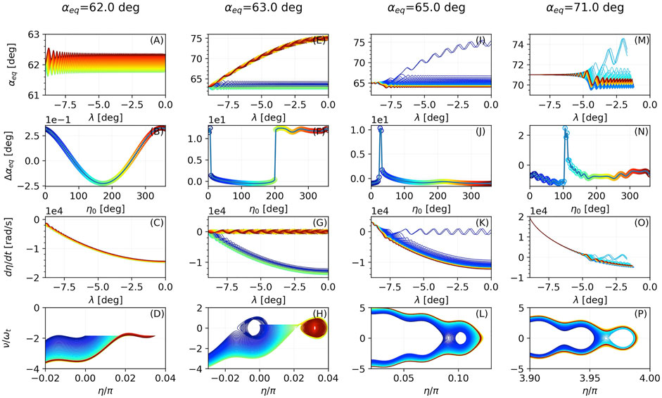
FIGURE 6. Evolution of α_eq along λ (A,E,I,M), distribution of Δα_eq with respect to the initial wave-particle phase η₀ (B,F,J,N), derivative of wave-particle phase η along λ (C,G,K,O) and electron trajectories in the ν-η plane (D,H,L,P) for different values of equatorial pitch angle.

As part of the third step of the parametric study, in Figure 7 we present wave-particle interaction results for electrons with energy in the range from 90 to 270 keV, while keeping the rest of the simulation parameters as in the baseline simulation presented above. We note that, as the energy becomes higher, the resonance point moves to higher latitudes. For the case of 90 keV, the resonance point is beyond the equator, and as the electrons are simulated until they reach the equator, no resonance is observed to occur. The resonance point is within the latitudinal range of our simulations for the range around 100–270 keV. Another feature of the simulations is that, as the energy becomes higher, fewer electrons become phase trapped, but with higher pitch angle scattering: thus, for 140 keV electrons the maximum pitch angle change is around 5°, for 200 keV electrons around 8° and for 270 keV electrons around 11°. Also, the oscillation of the pitch angle of trapped electrons becomes smaller with higher energy.

FIGURE 7

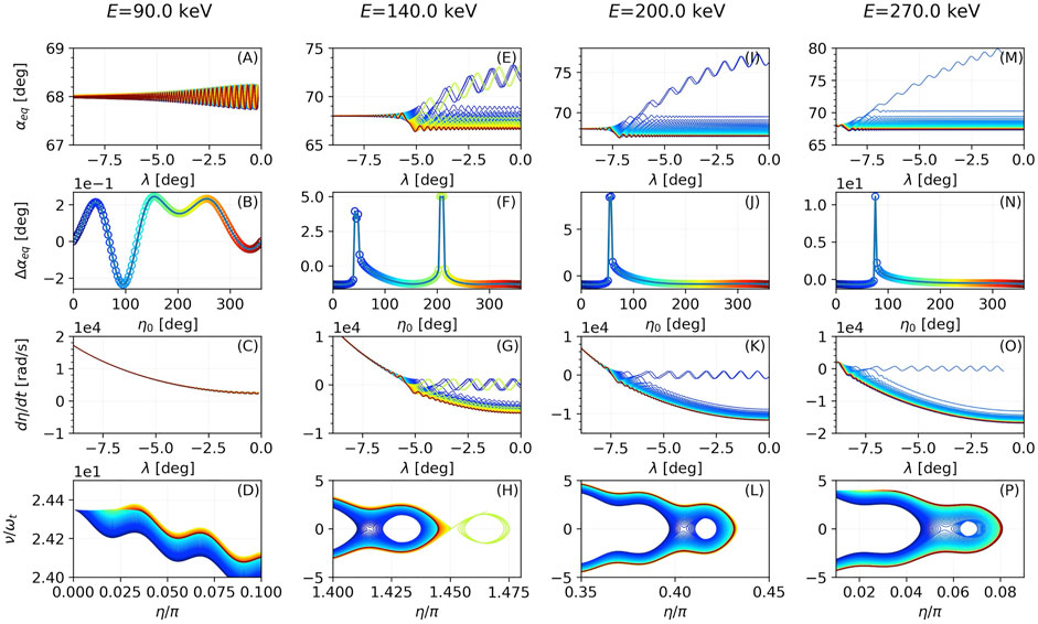
FIGURE 7. Evolution of α_eq along λ (A,E,I,M), distribution of Δα_eq with respect to the initial wave-particle phase η₀ (B,F,J,N), derivative of wave-particle phase η along λ (C,G,K,O) and electron trajectories in the ν-η plane (D,H,L,P) for different values of the electron energy.

Under the fourth step of the parametric study, we explore how the wave normal angle affects the nonlinear behaviour of the electrons. In all the simulations presented above, the waves have been considered to be parallel (i.e. ψ = 0 deg). The wave normal angle affects the resonance condition (Eq 47) through the parallel wave number k_‖ = k cos ψ. The upper limit of the wave normal angle for our simulations is defined by the resonance cone angle. Outside of the resonance cone no wave modes propagate and as ψ approaches the resonance cone angle, the wave number goes to infinity, or equivalently the wavelength goes to zero. By using WPIT. WaveProperties_mod.res_angle we calculate the resonance angle θ_res along the magnetic latitude and the results are presented in Figure 3C. For our latitudinal range of interest (−9 to 0°), θ_res ranges from around 73–75°. In order to ensure that the wave normal angle is inside the resonance cone for all the latitudes of interest, we set the upper limit of the wave normal angle at 72°. In Figure 8 we present the results for ψ = 1^o, 50^o, 60^o, 72^o. For the case of ψ = 1^o, the results are similar to the baseline case with some electrons experiencing phase trapping and some experiencing weak phase bunching. As the wave becomes more oblique, the nonlinear effects begin to decline. Thus, for ψ = 50° only three electrons are phase trapped and for ψ = 60° only weak phase bunching occurs. As the wave normal angle approaches the resonance cone angle (ψ = 72^o) the interactions become linear. Thus for the parameters of our simulation, the interactions become progressively more linear as the wave becomes more oblique.

FIGURE 8

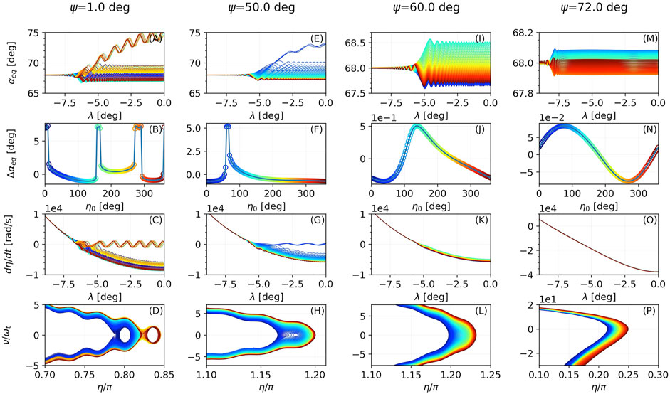
FIGURE 8. Evolution of α_eq along λ (A,E,I,M), distribution of Δα_eq with respect to the initial wave-particle phase η₀ (B,F,J,N), derivative of wave-particle phase η along λ (C,G,K,O) and electron trajectories in the ν-η plane (D,H,L,P) for different values of the wave normal angle.

In the baseline simulation we used an equatorial electron density of 10 × 10⁶ m⁻³ based on Bortnik et al. (2008). In Figure 9 we present results for interactions under different equatorial electron densities. Equatorial electron density affects the location of the resonance point, in the sense that as the electron density is increased, the resonance point moves to lower latitudes. For the case of n_eq = 25 × 10⁶ m⁻³, the electrons start at the resonance point as can be seen in Figure 9C, on the other hand for densities n_eq < 5 × 10⁶ m⁻³ the resonance point is located higher than the equator. In the case of n_eq = 25 × 10⁶ m⁻³ only strong phase bunching has occurred with none of the electrons trapped. If we compare the cases of n_eq = 12 × 10⁶ m⁻³, n_eq = 7 × 10⁶ m⁻³ and the baseline simulation (n_eq = 10 × 10⁶ m⁻³), we conclude that as the electron density becomes smaller more electrons become phase trapped, though with progressively lower maximum pitch angle scattering.

FIGURE 9

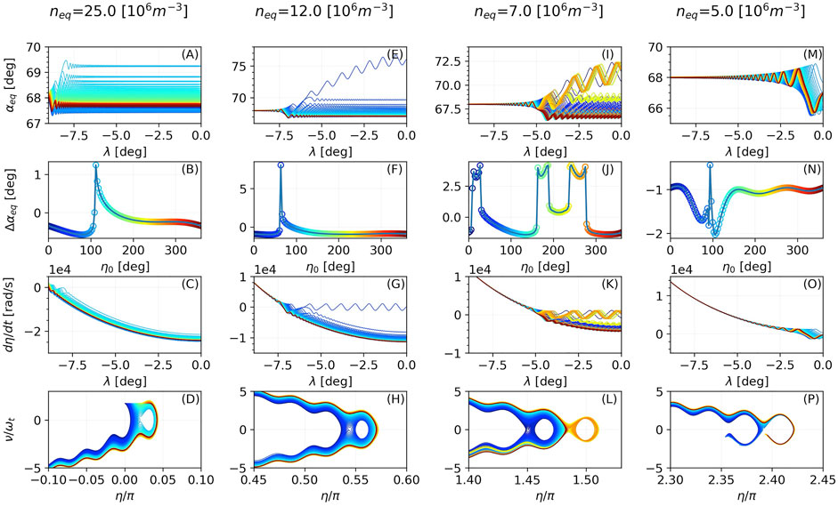
FIGURE 9. Evolution of α_eq along λ (A,E,I,M), distribution of Δα_eq with respect to the initial wave-particle phase η₀ (B,F,J,N), derivative of wave-particle phase η along λ (C,G,K,O) and electron trajectories in the ν-η plane (D,H,L,P) for different values of the equatorial electron density.

In Figure 10 we present results of the interactions with a wave of frequency in the range 1.4–3 kHz. For the 1.4 kHz case, the resonance point is located beyond the equator so the electrons did not reach it. On the other hand for the 3 kHz case the resonance point is located below λ = −9° and again is missed by the electrons. Hence, it is concluded that the higher the frequency, the lower the location of the resonance point. As it can be inferred from our simulations, the wave field that could potentially drive nonlinear scattering, for the parameters defined in our simulation, has a rather wide bandwidth of 1.5 kHz (1.5–3 kHz).

FIGURE 10

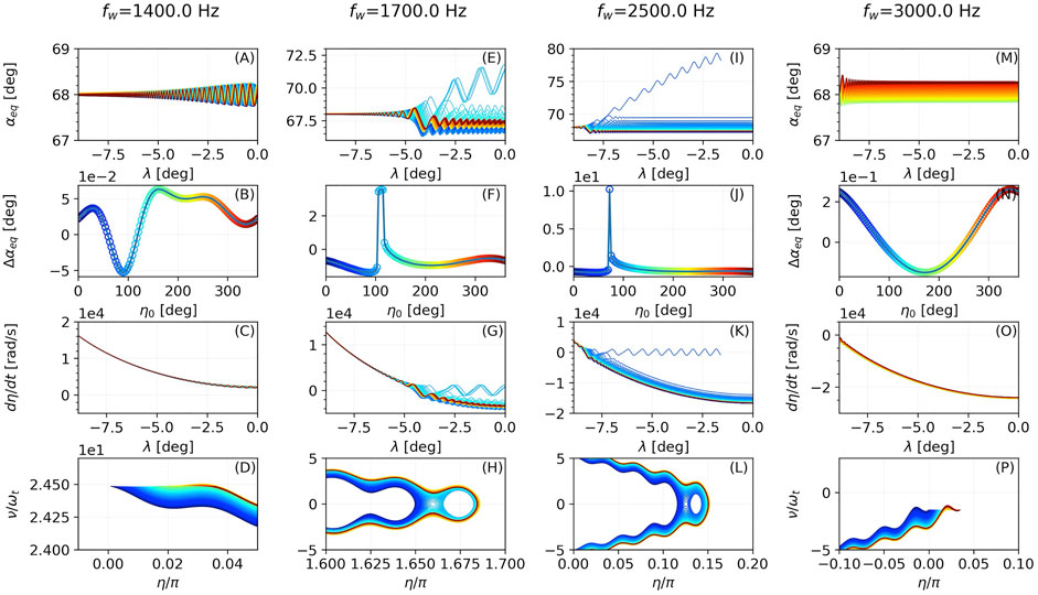
FIGURE 10. Evolution of α_eq along λ (A,E,I,M), distribution of Δα_eq with respect to the initial wave-particle phase η₀ (B,F,J,N), derivative of wave-particle phase η along λ (C,G,K,O) and electron trajectories in the ν-η plane (D,H,L,P) for different wave frequencies.

We have also explore the effect that variations in plasma composition have on the nonlinear behaviour of the electrons. The results are not presented here but can be found in WPIT_Results folder of the WPIT repository. No large discrepancies between the runs with different ion compositions were found, with the only difference consisting of slight shifts in η₀ of the phase-trapped populations.

4 Discussion

We have presented WPIT, an open source, Python-based toolset for the investigation of interactions of charged particles with very low frequency waves in Earth’s magnetosphere. WPIT is the first step, aiming to provide a unified code for the exploration of wave particle interactions inside the magnetosphere. With the ever-increasing interest of the science community on wave particles interactions, WPIT comprises a useful tool for both theoretical analyses and quantitative assessments of wave-particle interaction processes.

In Section 3, we presented results of the use of the code, by simulating the interactions of electrons with whistler-mode waves. We performed a parametric study by adjusting parameters such as the amplitude of the wave magnetic field, the equatorial pitch angle, the electron energy, the wave normal angle, the equatorial electron density, the wave frequency, and the electron and ion composition, and we examined the sensitivity of the onset of nonlinear effects for each case.

In terms of the amplitude of the wave magnetic field, we find that, in the simulations performed, there is a lower threshold in wave amplitude for the appearance of nonlinearity in wave-particle interactions. WPIT enables the identification of this threshold, based also on the entire parameter space that is explored. The pitch angle was also found to greatly affect the resonance location, and also whether electrons will be phase trapped. We note that an expanded parametric study should include a wider range of initial latitudes for the electrons than was presented herein, so that pitch angle effects can be better quantified. WPIT enables such parametric studies to be pursued. In terms of the effect of electron energy, it is found that the resonance location in terms of latitude generally decreases as the electron energy increases. Extended parametric studies could include such an extended range of initial latitudes for the electrons.

With this study we presented the capabilities of WPIT modules for extensive analysis of wave particle interactions. A potential expansion of the parametric study presented herein would be to conduct extensive simulations for the characterisation of the dependence of nonlinear effects on each wave and particle characteristic. Another important aspect that we conclude from our simulations is the need for higher resolution wave-particle phase distributions for the investigation of nonlinear wave particle interactions. With the simulation code available in Jupyter Notebook format in WPIT repository, a user can be guided through the set up of the relevant simulations for the performance of such more detailed parametric studies.

The goal of WPIT is to provide an open-source toolset for wave-particle interaction simulations to the scientific community, and it is expected and envisioned that other researchers will be contributing extensively to future versions, greatly enhancing the functionalities and capabilities of WPIT. However, we note that, since the implementation of WPIT involves a long sequence of processes as described above, some of which involve complex equations that require extensive testing and proper application of the assumptions used, it is preferred that any potential new functionalities and additions to WPIT by other researchers are implemented after communication with the authors.

Further to the scientific analysis of wave-particle interactions that was presented, and related to the quantification of the effectiveness of waves to resonantly scatter electrons, a practical application of WPIT is related to investigations of optimal schemes for radiation belt remediation. This refers to the active removal of energetic electrons from the radiation belts for the protection of satellite systems: Energetic electrons originating either from the solar wind or from high-altitude nuclear explosions can severely damage satellites, particularly in Low-Earth Orbit (LEO) (see, e.g., Carlsten et al., 2019, and references therein). With the emergence of NewSpace mega-constellations (Zhang et al., 2022) and the shift of space usage to LEO satellites for a range of applications, naturally or artificially produced energetic electrons constitute a serious potential vulnerability. In order to provide means for addressing this vulnerability, various schemes have been proposed that can potentially remove trapped electrons from the radiation belts (e.g. Hoyt and Minor, 2005; Sauvaud et al., 2008; Shao et al., 2009; de Soria-Santacruz and Martinez-Sanchez, 2013). Amongst the most promising schemes is the use of Very Low Frequency (VLF) waves to scatter electrons and lead them to precipitate into the Earth’s atmosphere. WPIT provides an optimal simulation tool that enables quantifying the wave characteristics that can lead to particle scattering, as well as evaluating the effectiveness of the scattering mechanism. To this direction, future work on WPIT involves including a module for the calculation of in situ transmissions of VLF waves by user-defined antenna characteristics. With the inclusion of a module that calculates the near and far field of antennas in magnetospheric plasmas, and along with calculation of the generated wave field through ray tracing, WPIT can become a useful tool, not only for theoretical studies, but also for space missions targeting wave particle interactions, as well as for VLF transmitters immersed in magnetospheric plasmas and for investigations of the efficiency of radiation belt remediation schemes.

Data availability statement

The datasets presented in this study can be accessed from the WPIT online repository through the link: https://github.com/stourgai/WPIT.

Author contributions

ST wrote the WPIT code and performed the scientific analysis presented in the manuscript. TS contributed to conception and design of the study. ST and TS contributed to the scientific analysis of the simulation results. ST wrote the first draft of the manuscript. ST and TS contributed to manuscript revision, read, and approved the submitted version.

Funding

The research work was supported by the Hellenic Foundation for Research and Innovation (HFRI) under the HFRI PhD Fellowship grant (Fellowship Number: 400), and DUTH projects KE82372 and KE82875.

Conflict of interest

The authors declare that the research was conducted in the absence of any commercial or financial relationships that could be construed as a potential conflict of interest.

Publisher’s note

All claims expressed in this article are solely those of the authors and do not necessarily represent those of their affiliated organizations, or those of the publisher, the editors and the reviewers. Any product that may be evaluated in this article, or claim that may be made by its manufacturer, is not guaranteed or endorsed by the publisher.

Supplementary material

The Supplementary Material for this article can be found online at: https://www.frontiersin.org/articles/10.3389/fspas.2022.1005598/full#supplementary-material.

Supplementary Figure S1 | Evolution of electron’s equatorial pitch angle α_eq along magnetic latitude λ. Reproduction of Figure 2i of Bortnik et al. (2008) with WPIT’s “Nonlinear interaction of energetic electrons with large amplitude chorus.ipynb”.

Supplementary Figure S2 | Evolution of electron energy along magnetic latitude λ. Reproduction of Figure 2j of Bortnik et al. (2008) with WPIT’s “Nonlinear interaction of energetic electrons with large amplitude chorus.ipynb”.

Supplementary Figure S3 | Distribution of total pitch angle change ∆α_eq with respect to the initial wave-particle phase η₀. Reproduction of Figure 2k of Bortnik et al. (2008) with “WPIT’s Nonlinear interaction of energetic electrons with large amplitude chorus.ipynb”.

Supplementary Figure S4 | Evolution of electron's equatorial pitch angle α_eq along magnetic latitude λ. Reproduction of Figure 4a of Albert and Bortnik (2009) with WPIT’s “Nonlinear interaction of radiation belt electrons with electromagnetic ion cyclotron waves.ipynb”.

Supplementary Figure S5 | Evolution of electron’s energy along magnetic latitude λ. Reproduction of Figure 4b of Albert and Bortnik (2009) with WPIT’s “Nonlinear interaction of radiation belt electrons with electromagnetic ion cyclotron waves.ipynb”.

Supplementary Figure S6 | Distribution of total pitch angle change ∆α_eq with respect to the initial wave-particle phase η₀. Reproduction of Figure 4c of Albert and Bortnik (2009) with WPIT’s “Nonlinear interaction of radiation belt electrons with electromagnetic ion cyclotron waves.ipynb”.

Supplementary Figure S7 | Evolution of electron’s equatorial pitch angle α_eq along magnetic latitude λ. Reproduction of Figure 12a of Su et al. (2012) with WPIT’s “Bounce-averaged advection and diffusion coefficients formonochromatic electromagnetic ion cyclotron wave Comparison between test-particle and quasi-linear models.ipynb”.

Supplementary Figure S8 | Distribution of total pitch angle change ∆α_eq with respect to the initial wave-particle phase η₀. Reproduction of Figure 12b of Su et al. (2012) with WPIT’s “Bounce-averaged advection and diffusion coefficients for monochromatic electromagnetic ion cyclotron wave Comparison between test-particle and quasi-linear models.ipynb”.

Supplementary Figure S9 | Evolution of ion’s equatorial pitch angle α_eq along magnetic latitude λ. Reproduction of Figure 3f of Su et al. (2014) with WPIT’s “Latitudinal dependence of nonlinear interaction between electromagnetic ion cyclotron wave and terrestrial ring current ions.ipynb“.

Supplementary Figure S10 | Evolution of ion energy along magnetic latitude λ. Reproduction of Figure 3g of Su et al. (2014) with WPIT’s “Latitudinal dependence of nonlinear interaction between electromagnetic ion cyclotron wave and terrestrial ring current ions.ipynb”.

Supplementary Figure S11 | Nonlinear parameter S as a function of magnetic latitude λ. Reproduction of Figure 3i of Su et al. (2014) with WPIT’s “Latitudinal dependence of nonlinear interaction between electromagnetic ion cyclotron wave and terrestrial ring current ions.ipynb”.

Supplementary Figure S12 | Distribution of total pitch angle change ∆α_eq with respect to the initial wave-particle phase η₀. Reproduction of Figure 4c of Su et al. (2014) with WPIT’s “Latitudinal dependence of nonlinear interaction between electromagnetic ion cyclotron wave and terrestrial ring current ions.ipynb”.

Supplementary Figure S13 | Electron trajectories in ν-η and η-λ planes for interactions with 1pT wave. The interactions are linear (no phase trapping or phase bunching).

Supplementary Figure S14 | Electron trajectories in ν-η and η-λ planes for interactions with 10pT wave. Weak phase bunching is present (black arrows).

Supplementary Figure S15 | Electron trajectories in ν-η and η-λ planes for interactions with 35pT wave. Both phase trapping and phase bunching are present (black arrows).

References

Albert, J., and Bortnik, J. (2009). Nonlinear interaction of radiation belt electrons with electromagnetic ion cyclotron waves. Geophys. Res. Lett. 36, L12110. doi:10.1029/2009gl038904

CrossRef Full Text | Google Scholar

Albert, J. (2005). Evaluation of quasi-linear diffusion coefficients for whistler mode waves in a plasma with arbitrary density ratio. J. Geophys. Res. 110, A03218. doi:10.1029/2004ja010844

CrossRef Full Text | Google Scholar

Albert, J. M., Tao, X., and Bortnik, J. (2012). “Aspects of nonlinear wave-particle interactions,” in Dynamics of the Earth’s radiation belts and inner magnetosphere (Washington: AGU), 199, 255–264.

Google Scholar

Allanson, O., Watt, C., Ratcliffe, H., Allison, H. J., Meredith, N., Bentley, S., et al. (2020). Particle-in-cell experiments examine electron diffusion by whistler-mode waves: 2. Quasi-linear and nonlinear dynamics. J. Geophys. Res. Space Phys. 125, e2020JA027949. doi:10.1029/2020ja027949

CrossRef Full Text | Google Scholar

Allanson, O., Watt, C., Ratcliffe, H., Meredith, N., Allison, H. J., Bentley, S., et al. (2019). Particle-in-cell experiments examine electron diffusion by whistler-mode waves: 1. Benchmarking with a cold plasma. J. Geophys. Res. Space Phys. 124, 8893–8912. doi:10.1029/2019ja027088

CrossRef Full Text | Google Scholar

Appleton, E. V. (1932). Wireless studies of the ionosphere. Proc. Inst. Electr. Eng. 7, 257–265. doi:10.1049/pws.1932.0027

CrossRef Full Text | Google Scholar

Artemyev, A., Neishtadt, A., and Vasiliev, A. (2020). Mapping for nonlinear electron interaction with whistler-mode waves. Phys. Plasmas 27, 042902. doi:10.1063/1.5144477

CrossRef Full Text | Google Scholar

Artemyev, A., Vasiliev, A., Mourenas, D., Agapitov, O., and Krasnoselskikh, V. (2013). Nonlinear electron acceleration by oblique whistler waves: Landau resonance vs. cyclotron resonance. Phys. Plasmas 20, 122901. doi:10.1063/1.4836595

CrossRef Full Text | Google Scholar

Aubry, M., Bitoun, J., and Graff, P. (1970). Propagation and group velocity in a warm magnetoplasma. Radio Sci. 5, 635–645. doi:10.1029/rs005i003p00635

CrossRef Full Text | Google Scholar

Bell, T. F. (1984). The nonlinear gyroresonance interaction between energetic electrons and coherent vlf waves propagating at an arbitrary angle with respect to the Earth’s magnetic field. J. Geophys. Res. 89, 905–918. doi:10.1029/ja089ia02p00905

CrossRef Full Text | Google Scholar

Bell, T. F. (1986). The wave magnetic field amplitude threshold for nonlinear trapping of energetic gyroresonant and landau resonant electrons by nonducted vlf waves in the magnetosphere. J. Geophys. Res. 91, 4365–4379. doi:10.1029/ja091ia04p04365

CrossRef Full Text | Google Scholar

Bell, T., Inan, U., Bortnik, J., and Scudder, J. (2002). The landau damping of magnetospherically reflected whistlers within the plasmasphere. Geophys. Res. Lett. 29, 23-1–23-4. doi:10.1029/2002gl014752

CrossRef Full Text | Google Scholar

Bortnik, J., Inan, U. S., and Bell, T. F. (2003b). Energy distribution and lifetime of magnetospherically reflecting whistlers in the plasmasphere. J. Geophys. Res. 108 (A5), 1199. doi:10.1029/2002ja009316

CrossRef Full Text | Google Scholar

Bortnik, J., Inan, U. S., and Bell, T. F. (2006). Landau damping and resultant unidirectional propagation of chorus waves. Geophys. Res. Lett. 33, L03102. doi:10.1029/2005gl024553

CrossRef Full Text | Google Scholar

Bortnik, J. (2004). Precipitation of radiation belt electrons by lightning-generated magnetospherically reflecting whistler waves. Stanford, California: stanford university.

Google Scholar

Bortnik, J., Thorne, R., and Inan, U. S. (2008). Nonlinear interaction of energetic electrons with large amplitude chorus. Geophys. Res. Lett. 35, L21102. doi:10.1029/2008gl035500

CrossRef Full Text | Google Scholar

Bortnik, J., Thorne, R. M., and Meredith, N. (2007). Modeling the propagation characteristics of chorus using crres suprathermal electron fluxes. J. Geophys. Res. 112, A08204. doi:10.1029/2006ja012237

CrossRef Full Text | Google Scholar

Bortnik, J., Thorne, R., Ni, B., and Li, J. (2015). Analytical approximation of transit time scattering due to magnetosonic waves. Geophys. Res. Lett. 42, 1318–1325. doi:10.1002/2014gl062710

CrossRef Full Text | Google Scholar

Brinca, A. (1972). On the stability of obliquely propagating whistlers. J. Geophys. Res. 77, 3495–3507. doi:10.1029/ja077i019p03495

CrossRef Full Text | Google Scholar

Carlsten, B. E., Colestock, P. L., Cunningham, G. S., Delzanno, G. L., Dors, E. E., Holloway, M. A., et al. (2019). Radiation-belt remediation using space-based antennas and electron beams. IEEE Trans. Plasma Sci. IEEE Nucl. Plasma Sci. Soc. 47, 2045–2063. doi:10.1109/tps.2019.2910829

CrossRef Full Text | Google Scholar

Carpenter, D., and Anderson, R. (1992). An isee/whistler model of equatorial electron density in the magnetosphere. J. Geophys. Res. 97, 1097–1108. doi:10.1029/91ja01548

CrossRef Full Text | Google Scholar

Chang, S., Ni, B., Bortnik, J., Zhou, C., Zhao, Z., Li, J., et al. (2014). Resonant scattering of energetic electrons in the plasmasphere by monotonic whistler-mode waves artificially generated by ionospheric modification. Ann. Geophys. 32, 507–518. doi:10.5194/angeo-32-507-2014

CrossRef Full Text | Google Scholar

Chen, L., Bortnik, J., Thorne, R. M., Horne, R. B., and Jordanova, V. K. (2009). Three-dimensional ray tracing of vlf waves in a magnetospheric environment containing a plasmaspheric plume. Geophys. Res. Lett. 36, L22101. doi:10.1029/2009gl040451

CrossRef Full Text | Google Scholar

de Soria-Santacruz, M., and Martinez-Sanchez, M. (2013). Electromagnetic ion cyclotron waves for radiation belt remediation applications. IEEE Trans. Plasma Sci. IEEE Nucl. Plasma Sci. Soc. 41, 3329–3337. doi:10.1109/tps.2013.2260181

CrossRef Full Text | Google Scholar

Denton, R., Goldstein, J., and Menietti, J. (2002). Field line dependence of magnetospheric electron density. Geophys. Res. Lett. 29, 58-1–58-4. doi:10.1029/2002gl015963

CrossRef Full Text | Google Scholar

Fu, S., Yi, J., Ni, B., Zhou, R., Hu, Z., Cao, X., et al. (2020). Combined scattering of radiation belt electrons by low-frequency hiss: Cyclotron, landau, and bounce resonances. Geophys. Res. Lett. 47, e2020GL086963. doi:10.1029/2020gl086963

CrossRef Full Text | Google Scholar

Gan, L., Li, W., Ma, Q., Albert, J., Artemyev, A., and Bortnik, J. (2020). Nonlinear interactions between radiation belt electrons and chorus waves: Dependence on wave amplitude modulation. Geophys. Res. Lett. 47, e2019GL085987. doi:10.1029/2019gl085987

CrossRef Full Text | Google Scholar

Gao, Z., Zhu, H., Zhang, L., Zhou, Q., Yang, C., and Xiao, F. (2014). Test particle simulations of interaction between monochromatic chorus waves and radiation belt relativistic electrons. Astrophys. Space Sci. 351, 427–434. doi:10.1007/s10509-014-1859-1

CrossRef Full Text | Google Scholar

Ginet, G. P., and Albert, J. M. (1991). Test particle motion in the cyclotron resonance regime. Phys. Fluids B Plasma Phys. 3, 2994–3012. doi:10.1063/1.859778

CrossRef Full Text | Google Scholar

Golden, D., Spasojevic, M., Foust, F., Lehtinen, N., Meredith, N. P., and Inan, U. (2010). Role of the plasmapause in dictating the ground accessibility of elf/vlf chorus. J. Geophys. Res. 115. doi:10.1029/2010ja015955

CrossRef Full Text | Google Scholar

Horne, R. B., and Thorne, R. M. (1993). On the preferred source location for the convective amplification of ion cyclotron waves. J. Geophys. Res. 98, 9233–9247. doi:10.1029/92ja02972

CrossRef Full Text | Google Scholar

Horne, R. B., and Thorne, R. M. (1998). Potential waves for relativistic electron scattering and stochastic acceleration during magnetic storms. Geophys. Res. Lett. 25, 3011–3014. doi:10.1029/98gl01002

CrossRef Full Text | Google Scholar

Horne, R. B. (2015). Trapping and acceleration of upflowing ionospheric electrons in the magnetosphere by electrostatic electron cyclotron harmonic waves. Geophys. Res. Lett. 42, 975–980. doi:10.1002/2014gl062406

CrossRef Full Text | Google Scholar

Hoyt, R. P., and Minor, B. M. (2005). “Remediation of radiation belts using electrostatic tether structures,” in 2005 IEEE Aerospace Conference, Big Sky, MT, USA, 05-12 March 2005 (Piscataway, NJ: IEEE), 583–594.

CrossRef Full Text | Google Scholar

Huang, H., Gao, X.-T., Wang, X.-G., and Wang, Z.-B. (2017). Electron acceleration and diffusion in the gyrophase space by low-frequency electromagnetic waves. IEEE Trans. Plasma Sci. IEEE Nucl. Plasma Sci. Soc. 46, 225–229. doi:10.1109/tps.2017.2771277

CrossRef Full Text | Google Scholar

Inan, U. S. (1987). Gyroresonant pitch angle scattering by coherent and incoherent whistler mode waves in the magnetosphere. J. Geophys. Res. 92, 127–142. doi:10.1029/ja092ia01p00127

CrossRef Full Text | Google Scholar

Inan, U. S., and Tkalcevic, S. (1982). Nonlinear equations of motion for landau resonance interactions with a whistler mode wave. J. Geophys. Res. 87, 2363–2367. doi:10.1029/ja087ia04p02363

CrossRef Full Text | Google Scholar

Jasna, D., Inan, U. S., and Bell, T. F. (1992). Precipitation of suprathermal (100 ev) electrons by oblique whistler waves. Geophys. Res. Lett. 19, 1639–1642. doi:10.1029/92gl01811

CrossRef Full Text | Google Scholar

Jordanova, V., Albert, K. J., and Miyoshi, Y. (2008). Relativistic electron precipitation by emic waves from self-consistent global simulations. J. Geophys. Res. 113, A00A10. doi:10.1029/2008ja013239

CrossRef Full Text | Google Scholar

Karpman, V., Istomin, J. N., and Shklyar, D. (1975). Effects of nonlinear interaction of monochromatic waves with resonant particles in the inhomogeneous plasma. Phys. Scr. 11, 278–284. doi:10.1088/0031-8949/11/5/008

CrossRef Full Text | Google Scholar

Karpman, V., and Shklyar, D. (1977). Partcle precipitation caused by a single whistler-mode wave injected into the magnetosphere. Planet. Space Sci. 25, 395–403. doi:10.1016/0032-0633(77)90055-1

CrossRef Full Text | Google Scholar

Kennel, C. (1966). Low-frequency whistler mode. Phys. Fluids 9, 2190–2202. doi:10.1063/1.1761588

CrossRef Full Text | Google Scholar

Kimura, I. (1966). Effects of ions on whistler-mode ray tracing. Radio Sci. 1, 269–284. doi:10.1002/rds196613269

CrossRef Full Text | Google Scholar

Kivelson, M. G., Kivelson, M. G., and Russell, C. T. (1995). Introduction to space physics. Cambridge, United Kingdom: Cambridge University Press.

Google Scholar

Kivelson, M. (2005). Transport and acceleration of plasma in the magnetospheres of Earth and jupiter and expectations for saturn. Adv. Space Res. 36, 2077–2089. doi:10.1016/j.asr.2005.05.104

CrossRef Full Text | Google Scholar

Koskinen, H. E., and Kilpua, E. K. (2022). “Particle source and loss processes,” in Physics of Earth’s radiation belts (Cham, Switzerland: Springer), 159–211.

CrossRef Full Text | Google Scholar

Kulkarni, P., Gołkowski, M., Inan, U., and Bell, T. (2015). The effect of electron and ion temperature on the refractive index surface of 1–10 khz whistler mode waves in the inner magnetosphere. J. Geophys. Res. Space Phys. 120, 581–591. doi:10.1002/2014ja020669

CrossRef Full Text | Google Scholar

Kulkarni, P., Inan, U. S., and Bell, T. F. (2008). Energetic electron precipitation induced by space based vlf transmitters. J. Geophys. Res. 113. doi:10.1029/2008ja013120

CrossRef Full Text | Google Scholar

Kulkarni, P., Inan, U. S., and Bell, T. F. (2006). Whistler mode illumination of the plasmaspheric resonant cavity via in situ injection of elf/vlf waves. J. Geophys. Res. 111, A10215. doi:10.1029/2006ja011654

CrossRef Full Text | Google Scholar

Lauben, D. S., Inan, U. S., and Bell, T. F. (2001). Precipitation of radiation belt electrons induced by obliquely propagating lightning-generated whistlers. J. Geophys. Res. 106, 29745–29770. doi:10.1029/1999ja000155

CrossRef Full Text | Google Scholar

Laval, G., and Pellat, R. (1970). Particle acceleration by electrostatic waves propagating in an inhomogeneous plasma. J. Geophys. Res. 75, 3255–3256. doi:10.1029/ja075i016p03255

CrossRef Full Text | Google Scholar

Lee, D.-Y., Kim, K.-C., and Choi, C.-R. (2020). Nonlinear scattering of 90 pitch angle electrons in the outer radiation belt by large-amplitude emic waves. Geophys. Res. Lett. 47, e2019GL086738. doi:10.1029/2019gl086738

CrossRef Full Text | Google Scholar

Li, J., Bortnik, J., Xie, L., Pu, Z., Chen, L., Ni, B., et al. (2015). Comparison of formulas for resonant interactions between energetic electrons and oblique whistler-mode waves. Phys. Plasmas 22, 052902. doi:10.1063/1.4914852

CrossRef Full Text | Google Scholar

Liu, K., Winske, D., Gary, S. P., and Reeves, G. D. (2012). Relativistic electron scattering by large amplitude electromagnetic ion cyclotron waves: The role of phase bunching and trapping. J. Geophys. Res. 117. doi:10.1029/2011ja017476

CrossRef Full Text | Google Scholar

Maxworth, A., and Gołkowski, M. (2017). Magnetospheric whistler mode ray tracing in a warm background plasma with finite electron and ion temperature. J. Geophys. Res. Space Phys. 122, 7323–7335. doi:10.1002/2016ja023546

CrossRef Full Text | Google Scholar

Maxworth, A., Gołkowski, M., Malaspina, D., and Jaynes, A. (2020). Raytracing study of source regions of whistler mode wave power distribution relative to the plasmapause. J. Geophys. Res. Space Phys. 125, e2019JA027154. doi:10.1029/2019ja027154

CrossRef Full Text | Google Scholar

Nunn, D. (1974). A self-consistent theory of triggered vlf emissions. Planet. Space Sci. 22, 349–378. doi:10.1016/0032-0633(74)90070-1

CrossRef Full Text | Google Scholar

Nunn, D., and Omura, Y. (2015). A computational and theoretical investigation of nonlinear wave-particle interactions in oblique whistlers. J. Geophys. Res. Space Phys. 120, 2890–2911. doi:10.1002/2014JA020898

CrossRef Full Text | Google Scholar

Ozhogin, P., Tu, J., Song, P., and Reinisch, B. (2012). Field-aligned distribution of the plasmaspheric electron density: An empirical model derived from the image rpi measurements. J. Geophys. Res. 117. doi:10.1029/2011ja017330

CrossRef Full Text | Google Scholar

Öztürk, M. K. (2012). Trajectories of charged particles trapped in Earth’s magnetic field. Am. J. Phys. 80, 420–428. doi:10.1119/1.3684537

CrossRef Full Text | Google Scholar

Parks, G. K. (1991). Physics of space plasmas. An introduction. Redwood City, CA: Addison-Wesley Publishing Co..

Google Scholar

Sauvaud, J.-A., Maggiolo, R., Jacquey, C., Parrot, M., Berthelier, J.-J., Gamble, R., et al. (2008). Radiation belt electron precipitation due to vlf transmitters: Satellite observations. Geophys. Res. Lett. 35, L09101. doi:10.1029/2008gl033194

CrossRef Full Text | Google Scholar

Schulz, M., and Lanzerotti, L. J. (2012). Particle diffusion in the radiation belts, 7. Berlin, Germany: Springer Science & Business Media.

Google Scholar

Shao, X., Papadopoulos, K., and Sharma, A. (2009). Control of the energetic proton flux in the inner radiation belt by artificial means. J. Geophys. Res. 114, A07214. doi:10.1029/2009ja014066

CrossRef Full Text | Google Scholar

Sheeley, B., Moldwin, M., Rassoul, H., and Anderson, R. (2001). An empirical plasmasphere and trough density model: Crres observations. J. Geophys. Res. 106, 25631–25641. doi:10.1029/2000JA000286

CrossRef Full Text | Google Scholar

Shklyar, D., and Matsumoto, H. (2009). Oblique whistler-mode waves in the inhomogeneous magnetospheric plasma: Resonant interactions with energetic charged particles. Surv. Geophys. 30, 55–104. doi:10.1007/s10712-009-9061-7

CrossRef Full Text | Google Scholar

Shprits, Y. Y. (2009). Potential waves for pitch-angle scattering of near-equatorially mirroring energetic electrons due to the violation of the second adiabatic invariant. Geophys. Res. Lett. 36, L12106. doi:10.1029/2009gl038322

CrossRef Full Text | Google Scholar

Sousa, A. P. (2018). Global and seasonal effects of lightning-induced electron precipitation. Stanford, California: Stanford University.

Google Scholar

Stix, T. H. (1992). Waves in plasmas. New York: Springer Science & Business Media.

Google Scholar

Su, Z., Zhu, H., Xiao, F., Zheng, H., Shen, C., Wang, Y., et al. (2012). Bounce-averaged advection and diffusion coefficients for monochromatic electromagnetic ion cyclotron wave: Comparison between test-particle and quasi-linear models. J. Geophys. Res. 117, A09222. doi:10.1029/2012ja017917

CrossRef Full Text | Google Scholar

Su, Z., Zhu, H., Xiao, F., Zheng, H., Shen, C., Wang, Y., et al. (2013). Latitudinal dependence of nonlinear interaction between electromagnetic ion cyclotron wave and radiation belt relativistic electrons. J. Geophys. Res. Space Phys. 118, 3188–3202. doi:10.1002/jgra.50289

CrossRef Full Text | Google Scholar

Su, Z., Zhu, H., Xiao, F., Zheng, H., Zhang, M., Liu, Y.-M., et al. (2014). Latitudinal dependence of nonlinear interaction between electromagnetic ion cyclotron wave and terrestrial ring current ions. Phys. Plasmas 21, 052310. doi:10.1063/1.4880036

CrossRef Full Text | Google Scholar

Summers, D. (2005). Quasi-linear diffusion coefficients for field-aligned electromagnetic waves with applications to the magnetosphere. J. Geophys. Res. 110, A08213. doi:10.1029/2005ja011159

CrossRef Full Text | Google Scholar

Summers, D., and Thorne, R. M. (2003). Relativistic electron pitch-angle scattering by electromagnetic ion cyclotron waves during geomagnetic storms. J. Geophys. Res. 108, 1143. doi:10.1029/2002ja009489

CrossRef Full Text | Google Scholar

Swanson, D. G. (2012). Plasma waves. New York: Elsevier.

Google Scholar

Tao, X., Bortnik, J., Albert, J. M., and Thorne, R. M. (2012). Comparison of bounce-averaged quasi-linear diffusion coefficients for parallel propagating whistler mode waves with test particle simulations. J. Geophys. Res. 117, A10205. doi:10.1029/2012ja017931

CrossRef Full Text | Google Scholar

Tao, X., and Bortnik, J. (2010). Nonlinear interactions between relativistic radiation belt electrons and oblique whistler mode waves. Nonlinear process. geophys. 17, 599–604. doi:10.5194/npg-17-599-2010

CrossRef Full Text | Google Scholar

Vainchtein, D., Zhang, X.-J., Artemyev, A., Mourenas, D., Angelopoulos, V., and Thorne, R. (2018). Evolution of electron distribution driven by nonlinear resonances with intense field-aligned chorus waves. JGR. Space Phys. 123, 8149–8169. doi:10.1029/2018ja025654

CrossRef Full Text | Google Scholar

Wang, B., Li, P., Huang, J., and Zhang, B. (2019). Nonlinear landau resonance between emic waves and cold electrons in the inner magnetosphere. Phys. Plasmas 26, 042903. doi:10.1063/1.5088374

CrossRef Full Text | Google Scholar

Wang, B., Su, Z., Zhang, Y., Shi, S., and Wang, G. (2016). Nonlinear landau resonant scattering of near equatorially mirroring radiation belt electrons by oblique emic waves. Geophys. Res. Lett. 43, 3628–3636. doi:10.1002/2016gl068467

CrossRef Full Text | Google Scholar

Zhang, J., Cai, Y., Xue, C., Xue, Z., and Cai, H. (2022). Leo mega constellations: Review of development, impact, surveillance, and governance. Space Sci. Technol. 2022, 9865174. doi:10.34133/2022/9865174

CrossRef Full Text | Google Scholar