GMAG: An open-source python package for ground-based magnetometers

Magnetometers are a key component of heliophysics research providing valuable insight into the dynamics of electromagnetic field regimes and their coupling throughout the solar system. On satellites, magnetometers provide detailed observations of the extension of the solar magnetic field into interplanetary space and of planetary environments. At Earth, magnetometers are deployed on the ground in extensive arrays spanning the polar cap, auroral and sub-auroral zone, mid- and low-latitudes and equatorial electrojet with nearly global coverage in azimuth (longitude or magnetic local time—MLT). These multipoint observations are used to diagnose both ionospheric and magnetospheric processes as well as the coupling between the solar wind and these two regimes at a fraction of the cost of in-situ instruments. Despite their utility in research, ground-based magnetometer data can be difficult to use due to a variety of file formats, multiple points of access for the data, and limited software. In this short article we review the Open-Source Python library GMAG which provides rapid access to ground-based magnetometer data from a number of arrays in a Pandas DataFrame, a common data format used throughout scientific research.

1 Introduction

Ground-based magnetometers have been used to study Earth’s geomagnetic environment for over a century (e.g., Birkeland 1908). In initially controversial but ground-breaking work Birkeland (1908) postulated that perturbations of the Earth’s magnetic field, observed by ground-based magnetometers, were driven by ionospheric currents connected to a system of currents flowing along Earth’s magnetic field lines into and out of the polar ionosphere. It wasn’t until the launch of spacecraft with onboard magnetometers in the 1960’s and 1970’s (e.g., Zmuda et al., 1966; Zmuda et al., 1967, and Iijima and Potemra 1976, Iijima and Potemra 1978) that Birkeland’s theory of field aligned currents was proven correct, paving the way for the study of heliophysics and studies solar wind-magnetosphere-ionosphere coupling. Today, the ionospheric current systems studied by Birkland are known as the auroral electrojets and the field aligned current systems he first postulated are now termed Birkeland currents.

Following Birkeland’s seminal work, ground-based magnetometers have become a fundamental tool in magnetospheric and ionospheric research providing the ability to study the spatio and temporal dynamics of Earth’s geomagnetic field driven by the coupling of the solar wind-magnetosphere-ionosphere systems. For example, Heppner (1954) demonstrated that the brightening of auroral arcs was strongly associated with perturbations of the Earth’s nightside magnetic field, highlighting a link between the aurora and the auroral electrojets during what is now known as the auroral substorm (Akasofu, 1964). Coordinated research utilizing multiple ground-based magnetometers expanded on these studies and allowed researchers to probe the spatial-temporal dynamics of processes coupling the magnetosphere and ionosphere. These studies have allowed researchers to determine the strength and location of the auroral electrojets (e.g., Rostoker and Phan, 1986), investigate the evolution of auroral substorms (e.g., McPherron, 1970), and define global magnetic indices to classify geomagnetic activity and which can be used as input to research and forecasting models (e.g., Kp, Dst, auroral electrojet indices; see Davis and Sugiura 1966; Iyemori 1990; Love and Remick, 2007, Kauristie, 2017, Yamazaki et al., 2022).

In the late 1970’s and early 1980’s the community began developing extended arrays and networks of ground-based magnetometers in response to International Solar-Terrestrial Physics Science (ISTP) (Jones 1986, see also Rostoker et al., 1995). Today, several magnetometer arrays exist spanning the polar cap, through the auroral oval, down to the equatorial electrojet and across the globe in longitude providing nearly continuous observations for as long as three solar cycles (e.g., Mann et al., 2008; Russell et al., 2008; Tanskanen 2009; Chulliat et al., 2017). These arrays allow researchers to conduct detailed studies of the spatial-temporal dynamics of the solar wind-magnetosphere-ionosphere system on global scales. This includes, for example: statistical (e.g. Mathie and Mann, 2000; Murphy et al., 2011) and event based studies of Ultra-low Frequency waves (e.g., Rae et al., 2019) which can be used in radiation belt modeling (e.g., Mann et al., 2016; Ozeke et al., 2017; Ma et al., 2018); studies of the spatial distribution and expansion of waves (e.g. Milling et al., 2008; Murphy et al., 2009), field aligned currents (e.g., Pulkkinen et al., 2003; Weygand et al., 2011), the substorm current wedge (e.g., Lester et al., 1983; Cramoysan et al., 1995), and geomagnetically induced currents (e.g., Pulkinen et al., 2005; Pulkinen et al., 2017; Smith et al., 2022); analysis of field line resonances (e.g., Mann et al., 2002; Rae et al., 2005); remote sensing of in-situ plasma properties (e.g., e.g., Mann et al., 2002; Rae et al., 2005); and magnetoseismology of ionospheric disturbances (e.g., Waters et al., 1996; Chi and Russell, 2005; Chi et al., 2013; Kale et al., 2009). For more examples see Mann et al. (2008), Russell et al. (2008), Menk and Waters (2013), Engebretson and Zesta (2017), and Murphy et al. (2022a)). Despite their utility in magnetospheric and ionospheric physics, the data from ground-based magnetometers can be difficult to use due to limited software, multiple file formats (e.g., text and CDF), varying sources and methods for obtaining the data, and varying temporal resolutions.

Recent community efforts to develop Open-Source software packages for scientists, including AstroPy (Robitaille et al., 2013; Price -Whelan et al., 2018), SunPy (Barnes et al., 2020), the THEMIS Data Analysis Software (TDAS) and its extension to the Space Physics Environment Data Analysis Software (SPEDAS) and pySPEDAS (Angelopoulos et al., 2019) have been extremely beneficial to the community. These resources reduce barriers to data access and provide well developed software that does not rely on the cost prohibitive licenses of programming languages such as MATLAB and IDL (see https://heliopython.org/projects/for an extensive list of Python packages for Heliophysics). In this short paper we detail the Open-Source Python package GMAG (Murphy, 2022b). GMAG is a simple package that provides access to over 200 ground-based magnetometers from multiple arrays in a Pandas DataFrame, a common data format used throughout data analysis and scientific research. We discuss installation of the package, the package modules, illustrate several examples, highlight the GMAG website, and discuss potential future extensions of the package.

2 GMAG

2.1 Python module

The GMAG Python package (Murphy, 2022b) provides access to just over 200 ground-based magnetometers (Figure 1) that are part of 12 arrays (Table 1). The GMAG directory and file structure is based on typical Python packages. The top-level directory is the GitHub repository GMAG. Within that directory is the Python package gmag, the docs directory, which contains the GMAG GitHub Pages website (below), and the notebooks directory which contains several examples. Figure 2 shows the structure of the GitHub directory and the GMAG package with short file descriptions. The main modules are the base gmag module and the arrays submodule (discussed below). GMAG can be installed by downloading or cloning the GitHub repository (https://github.com/kylermurphy/gmag) and using the single line of code pin install. from the terminal and within the GMAG directory, this also installs all GMAG requirements. Once installed the gmagrc_example should be renamed gmagrc and the variable data_dir, defining the local directory to download data, should be set by the user based on their preferences. GMAG is platform and operating system independent.

FIGURE 1

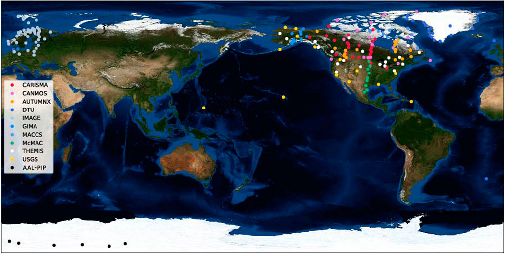
FIGURE 1. The geographic location of ground-based magnetometers that the GMAG package can download and load data for. The stations are color coded by their parent array (see legend and Table 1).

TABLE 1

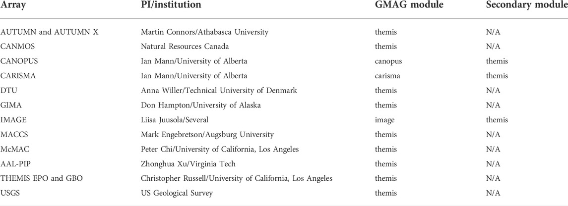
TABLE 1. The ground-based magnetometer arrays that can be accessed by the GMAG package.

FIGURE 2

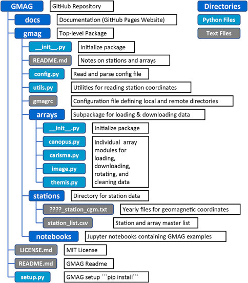
FIGURE 2. Structure of the GMAG GitHub Repository and gmag module.

The main gmag package provides a set of modules for parsing the configuration file and loading station data for various ground-based magnetometers (e.g., geographic, and altitude adjusted corrected geomagnetic coordinates - AACGM Burrell et al., 2018). The configuration file defines the local directory for downloading data, the variable data_dir and the web addresses of the data servers accessed by GMAG the variables ??_http where ?? is shorthand for the server. Though GMAG provides access to eleven ground-based arrays it uses only three data servers, the CARISMA, IMAGE, and THEMIS data servers. This is because the THEMIS server provides direct access to stations from all the magnetometer arrays listed in Table 1, which also provides redundancy for the CARISMA and IMAGE arrays. In addition to the configuration routines the main package contains the utils module, a set of utility functions for reading in station data, namely the coordinates for each station, and parent magnetometer array. The AACGM are calculated yearly using the Python packages igrf12 (Hirsch, 2021) and aacgmv2 (Burrell et al., 2018) and stored as text files in the format gmag/stations/????_station_cgm.txt, where ???? is the year, so they can be rapidly loaded. Note, installation of the igrf12 and aacgmv2 packages can be difficult; thus, the coordinate text files are generated using the notebook notebook/convert_coords.ipynb then saved to text files so to avoid difficulties of installing igrf12 and aacgmv2.

The arrays subpackage is the bulk of the gmag package and contains the functionality to list local and remote files, and download, load, clean, and rotate magnetometer data for the arrays listed in Table 1. The arrays subpackage is broken-down into four array specific modules, the carisma, image, themis, and canopus modules. The code is structured in this way as data is retrieved for each module from a different data server in a different file format. The carisma, canopus, and image modules load data in geographic XYZ coordinates where X is north, Y is east, and Z is vertical. These data are scrubbed using the clean() routine which replaces bad or poor quality data with not-a-number. Poor quality data are identified by flags (CARISMA and CANOPUS) or specific numbers (IMAGE) in the data files; currently no other cleaning (e.g., removal of spikes) is performed. These data are then rotated using the stations declination into local magnetic coordinates HDZ. Here H is the north, D is the east, and Z is the vertical magnetic field in nT. The declinations are loaded with gmag.utils.load_station_coor() from the yearly AACGM files stations/????_station_cgm.txt described above. The data loaded via the themis module has undergone extensive processing and is typically returned in local geomagnetic coordinates HDZ and so no additional processing or scrubbing is done to data loaded via the themis module. The canopus module loads CANOPUS data (CARISMA pre 1 April 2005) manually downloaded from the CARISMA website, as an easily accessible CANOPUS data server is not currently available, and performs the same data rotation and cleaning as the carisma module. The carisma, image, and themis modules also have the utility to download data files. Finally, the carisma, image, and canopus modules return data in both geographic and local geomagnetic coordinates (XYZ, HDZ).

For each array module data is loaded using the load() function. Data files are first searched for locally and then downloaded if no local files are found. For simplicity all the load() functions have the same basic parameters and will load observations from multiple stations for extended periods. The load() functions return both the magnetometer data and metadata for the loaded stations in well-defined Pandas DataFrames (e.g., clear, and descriptive column names). The download() functions allow users to download data without loading the data. GMAGs array modules and functions are summarized in Table 2. The CARISMA module downloads and loads 1 s resolution data, the IMAGE module downloads 10 s resolution. The resolution of data loaded by the THEMIS module varies with magnetometer array. In each case the returned metadata contains the temporal resolution of each station loaded. Note the CARISMA module does not currently load the 8 Hz data or the searchcoil data.

TABLE 2

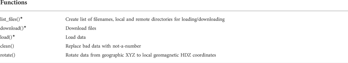
TABLE 2. List of function available for each of the arrays module. ^* function part of the THEMIS module.

It is important to note that there are a multitude of different data structures in Python, both built in and available via various packages. Python’s built-in data structures (lists, dictionaries, tuples, and sets) generally do not offer the utility required for scientific research and data analysis, e.g., data structure arithmetic such as adding or multiplying two series/vectors/arrays or matrix multiplication. Other packages, such as Numpy, Astropy, Sunpy, SpacePy, and xarray, offer data structures whose utility extends beyond Python’s built-in data structures and are more appropriate for research and data analysis. All these packages have their benefits. GMAG uses Pandas DataFrames as opposed to these other libraries as a DataFrame is ideal for handling both time-series and tabular data, further Pandas DataFrames provide built in functionality to rapidly plot and visualize data. The next section illustrates a number of use cases for the GMAG library.

2.2 GMAG, examples

The load() function in the carisma, canopus, image, and themis modules loads data from multiple magnetometer stations over extended periods. In general, analysis of short time periods or a small number of stations can be easily accomplished using the load() functions (e.g., case studies). For studies using a larger number of stations over extended periods (e.g., storms or statistical studies) data can first be downloaded using the download() function and subsequently loaded. The load and download functions use the station code/abbreviations. These codes can be found in the master station list (stations/station_list.csv), loaded via the utils module load_station_coor() and load_station_geo() routines (see example) or on the GMAG website (described below).

The Python code below demonstrates how to load data from each of the arrays modules (see comments for additional details).

# load CARISMA module

import gmag.arrays.carisma as carisma

# load 2 days of data from the ISLL and PINA

# using ndays to define the time span

df, meta = carisma.load(['ISLL','PINA'],'2012-01-01',ndays=2)

# using edate to define the end date

df, meta = carisma.load(['ISLL','PINA'],'2012-01-01',edate='2012-01-03')

# load IMAGE module

import gmag.arrays.image as image

# load 21 days of data from the AND station

df, meta = image.load('AND','2012-01-01',ndays=21)

# load THEMIS module

import gmag.arrays.themis as themis

# load 22 days of THEMIS data from the KUUJ station

# force download even if local files exist

df, meta = themis.load('KUUJ',sdate='2012-01-01',ndays=22, dl=True, force=True)

#load CANOPUS module

#load a single day of data from the ISLL station

import gmag.arrays.canopus as canopus

df, meta = canopus.load('ISLL',sdate='2001-01-01',ndays=1)

In each case the load() functions return data in a Pandas DataFrame. The index of the DataFrame is the timestamp and each column is a component of the magnetic field for each station loaded, in either geographic coordinates (XYZ), local geomagnetic coordinates (HDZ), or both. We use the timestamp as the index as this allows for rapid plotting in Pandas as well as combining observations with different cadences into a single DataFrame. The load() function also returns station metadata. Table 3 and Table 4 show examples of the data and metadata DataFrames returned by the load functions.

TABLE 3

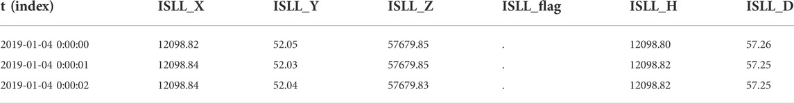
TABLE 3. Example of the returned DataFrame; in this case the carisma module. In the case of CARISMA data, the flag column identifies ok (.) and bad (x) data (bad data are replaced with not-a-number).

TABLE 4

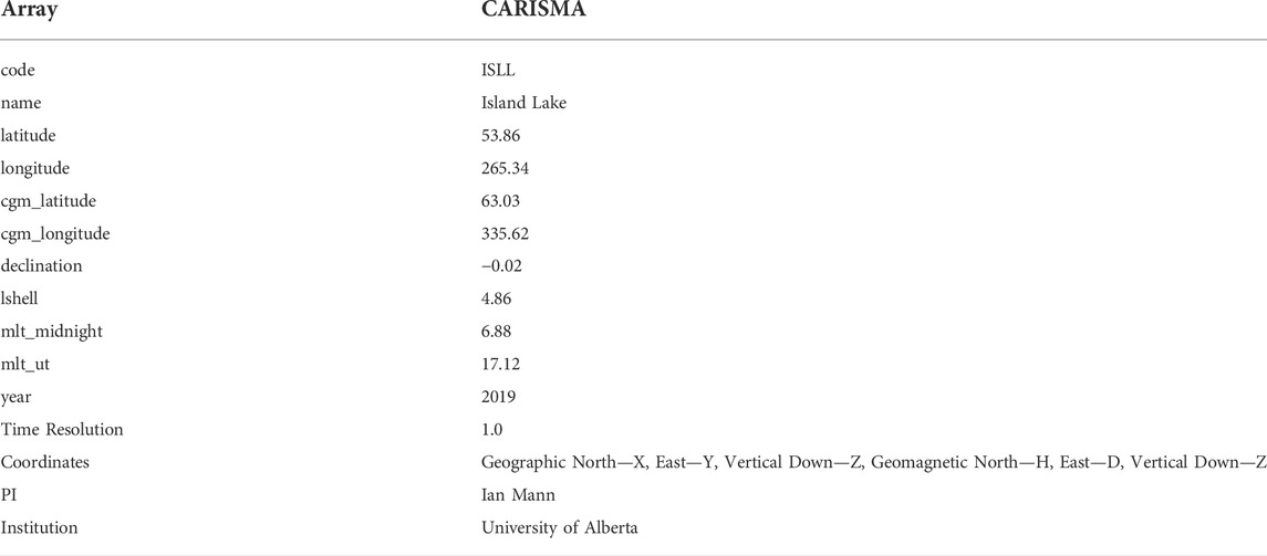
TABLE 4. Example metadata returned by the load functions.

The Magnetometer data DataFrame can be easily searched, accessed, and manipulated using a mix of Python’s and Panda’s indexing and DataFrame methods. DataFrames have the additional utility of being able to rapidly plot data using Pandas built in plotting and Matplotlib. The DataFrame can also be used with other Python packages such as Numpy, to rapidly produce publication quality plots or analyze the data using SciPy’s signal processing library or scikit-learn’s machine learning library. Figure 3 and the following block of code demonstrate how to rapidly load and plot data using the themis module during a substorm observed between 0530 and 0630 UT on 9 April 2011.

FIGURE 3

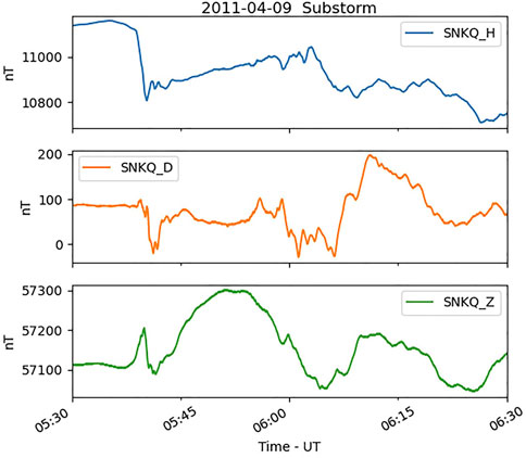
FIGURE 3. Example of a simple plot produced using Pandas built in plotting functionality highlighting a substorm observed by the SNKQ ground-based magnetometer station loaded using the themis module.

# import required modules

import numpy as np

import matplotlib.pyplot as plt

import gmag.arrays.themis as themis

# define start and end dates for plotting

sdate = '2011-04-09 05:30:00'

edate = '2011-04-09 06:30:00'

# load data

th_dat, th_meta = themis.load(['SNKQ'],sdate,ndays=1)

# plot all data in the DataFrame between

# sdate and edate

th_dat[sdate:edate].plot(ylabel='nT', xlabel='Time - UT', figsize=[6,6],subplots=True)

plt.title(sdate[0:11]+' Substorm',y=3.35)

More complex multi-station plots of specific components can also be rapidly generated with a few lines of code using list comprehension and chaining together Pandas and Numpy methods. Two examples are shown in Figure 4 and Figure 5 along with the accompanying code.

FIGURE 4

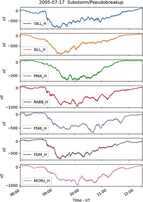
FIGURE 4. A multi-panel plot highlighting a substorm observed by select CARISMA magnetometer stations. Data was loaded using the carisma module and plotted using Pandas.

FIGURE 5

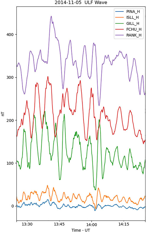
FIGURE 5. Multi-station stacked plot of a ULF wave observed by select CARISMA magnetometer stations that are a part of the Churchill line. The plot was generated using Pandas and Numpy.

Figure 4 shows the H component magnetic field (mean removed) from select CARISMA magnetometers in a multi-panel plot during a substorm observed on 17 July 2005. Figure 5 shows a stacked plot of a large amplitude Ultra-low Frequency (ULF) wave observed along the CARISMA Churchill line on 5 November 2011.

# Plot multi-panel plot of the H component

# magnetic field for select CARSIMA stations

# import required modules

import gmag.arrays.carisma as carisma

import numpy as np

import matplotlib.pyplot as plt

# define start and end date for plotting and loading

# assume a single day is loaded

sdate = '2005-07-17 08:00:00'

edate = '2005-07-17 12:30:00'

# define component to be plotted

comp='H'

# load data

car_dat,car_meta=carisma.load(['GILL','ISLL','PINA','RABB','FSMI','FSIM','MCMU'],sdate)

# find the correct columns of the DataFrame

p_col = [col for col in car_dat.columns if col[-1] == comp]

# plot the DataFrame between sdate and edate

# plot only p_col columns and subtract the mean from each column

# before plotting

car_dat[sdate:edate][p_col].subtract(car_dat[p_col].mean()).plot(ylabel='nT', xlabel='Time - UT', figsize=[6,10],subplots=True)

plt.title(sdate[0:11]+' Substorm/Pseudobreakup',y=8.25)

# import required modules

import gmag.arrays.carisma as carisma

import numpy as np

import matplotlib.pyplot as plt

# define start and end date for plotting

# use start date for loading data

sdate = '2014-11-05 13:25:00'

edate = '2014-11-05 14:25:00'

# define component for plotting

comp='H'

# load data

car_dat, car_meta=carisma.load(['PINA','ISLL','GILL','FCHU','RANK'],sdate)

# find the columns from the loaded DataFrame that have comp

# in the title, these are the columns that will be plotted

p_col = [col for col in car_dat.columns if col[-1] == comp]

# determine the shift to apply to each time series so that they don't

# overlap

# the shift is determined using the DataFrame returned by the describe()

# method which stores the DataFrame stats including max and min of each column

# only use columns from p_col and values between the start and end of plotting

# defined by sdate and edate

# the shift in the y direction is defined by 1.5 times the range of the series

y_shift = np.array([(val['max']-val['min'])/1.5 for col_h, val in car_dat[sdate:edate][p_col].describe().iteritems()])

# the cumsum() method determines the cumalitative sum up

# to each index

# the cumsum() ensures timeseries don't overlap

y_shift = (y_shift-y_shift.min()).cumsum()

# plot p_col columns of the data frame between sdate and edate

# subtract the mean from each time series and apply the y-shit

car_dat[sdate:edate][p_col].subtract(car_dat[sdate:edate][p_col].mean()-y_shift).plot(ylabel='nT', xlabel='Time - UT', figsize=[6,10])

plt.title(sdate[0:11]+' ULF Wave')

GMAG also allows extended periods of data to be downloaded using any of the download() functions. This allows users to download data without also loading the data into memory.

# download CARISMA

# data from ISLL

import gmag.arrays.carisma as carisma

carisma.download('ISLL','2012-01-01',ndays=21)

# download IMAGE data

import gmag.arrays.image as image

image.download('AND','2012-01-01',ndays=21)

# force download THEMIS data

import gmag.arrays.themis as themis

themis.download('KUUJ',sdate='2012-01-01',ndays=21, force= True)

Finally, the utils module provides two simple routines load_station_coor() and load_station_geo() for loading geographic and altitude adjusted corrected geomagnetic data for magnetometer stations. Both functions return data in DataFrame and in each case the col and param keywords can be used to filter a given DataFrame column by the param variable. Several examples are shown below. These functions can also be used in conjunction with the load() functions to load all stations from a particular magnetometer array.

from gmag import utils

#load geomagnetic data

#load all CARISMA station data for 2002

car_stn = utils.load_station_coor(param='CARISMA', col='array', year=2002)

#load GILL data from 2012

gill_stn = utils.load_station_coor(param='GILL', col='code', year=2012)

#load all data from 2012

all_stn = utils.load_station_coor(param='ALL', year=2012)

#load station geographic data

#load all CARISMA data

geo_stn = utils.load_station_geo(param='CARISMA', col='array')

#load all stations

all_stn = utils.load_station_geo(param='ALL')

A more complex example shows how to identify stations in a particular region of interest and then load data from those stations. This example can be modified to identify stations within a range of any combination of coordinates (e.g., L shell, longitude). Note, the GMAG GitHub repository includes a notebooks folder with several Jupyter Notebooks showing examples of the GMAG code, including those here.

import pandas as pd

from gmag import utils

import gmag.arrays.carisma as carisma

import gmag.arrays.image as image

import gmag.arrays.themis as themis

#find all stations between 18-24 MLT

#and L shells 6-8 during an event observed

#on 2018-01-01/04:00:00 UT

date = pd.to_datetime('2018-01-01/04:00:00')

mlt_min = 18

mlt_max = 24

l_min = 6

l_max = 8

#load all stations for date of interest

all_stn = utils.load_station_coor(param='*', year=date.year)

#calculate MLT of the stations for the date

#MLT at 0 UT is stored in the mlt_ut column

#mlt is then mlt at 0 UT plus current UT hour

all_stn['mlt'] = (all_stn['mlt_ut']+date.hour) % 24

#create masks for the mlt and lshell regions

mlt_mask = (all_stn['mlt'] >= mlt_min) & (all_stn['mlt'] <= mlt_max)

l_mask = (all_stn['lshell'] >= l_min) & (all_stn['lshell'] <= l_max)

#create masks for the arrays

car_mask = all_stn['array'] == 'CARISMA'

img_mask = all_stn['array'] == 'IMAGE'

#identify stations from each array

car_stn = all_stn[car_mask & mlt_mask & l_mask]

img_stn = all_stn[img_mask & mlt_mask & l_mask]

# ∼ is bitwise negation, not image or carisma (1 if 0, 0 if 1)

thm_stn = all_stn[∼img_mask & ∼car_mask & mlt_mask & l_mask]

#create an empty DataFrames

mag_meta = pd.DataFrame()

mag_data = pd.DataFrame()

#loop through stations and load data

for stn in [car_stn, img_stn, thm_stn]:

 #skip if no stations were identified

 if stn.shape[0] == 0:

   continue

 elif stn['array'].iloc[0] == 'CARISMA':

 l_dat, l_meta = carisma.load(car_stn['code'],date,ndays=1,drop_flag=True)

 elif stn['array'].iloc[0] == 'IMAGE':

 l_dat, l_meta = image.load(img_stn['code'],date,ndays=1,drop_flag=True)

 else:

 l_dat, l_meta = themis.load(thm_stn['code'],date,ndays=1)

# add loaded data to

mag_data = mag_data.join(l_dat,how='outer')

mag_meta = pd.concat([mag_meta,l_meta], axis=0, sort=False, ignore_index=True)

2.3 GMAG website

The GMAG website is located at https://kylermurphy.github.io/gmag/. The website provides simple and up to date documentation for the GMAG package as well as quick access to array and magnetometer station information. The array page includes a list of magnetometer arrays that can be accessed by GMAG, links to webpages and data access, as well as the acknowledgements and a link to the Terms and Conditions of Use (if available). The stations page includes a map of all stations, a table of the station’s geographic coordinates, and links to tables of the station’s AACGM coordinates. The tables are searchable allowing researchers to rapidly find information on each magnetometer array and their stations (e.g., L-shells). Finally, the examples page includes various usage examples for the package.

3 Conclusion and future possibilities

Ground-based magnetometers are a corner stone of heliophysics research. Compared to flight hardware, ground-based magnetometers are less cost-prohibitive, and are easier to deploy and maintain. This allows extensive networks of ground-based magnetometers to be deployed to study the global spatial-temporal dynamics of ULF waves (Mann et al., 2002), ionospheric and magnetospheric current systems (Weygand et al., 2011), substorms (Murphy et al., 2009), storms (Rae et al., 2019), radiation belt dynamics (Ozeke et al., 2017), or magnetosphere plasma distributions (Chi et al., 2005). Generally, these networks are deployed by individual PIs and research groups from various research institutions and Universities across the world. This allows for many stations to be deployed around the globe; however, this also generally means that no common ground-based magnetometer framework exists, for example, data format, cadence, access point and method, that allows researchers to easily and rapidly access high-resolution near real-time data.

Recent work has begun unifying ground-based magnetometer data, providing a common data format, access point, and software to access the data. The recently updated PySPEDAS Python package now includes access to ground-based magnetometer data from the THEMIS data server via PyTplot (the Python counterpart to SPEDAS’s IDL tplot routine) (Angelopoulos et al., 2019). The SuperMAG program provides ground-based magnetometer data from several magnetometer arrays in a common data format (Gjerlov, 2012); however, at the time of this writing, access to high cadence data via a simplified Python package is limited. Further, SuperMAG receives high resolution data on delayed schedule. Both the PySPEDAS and SuperMAG Python packages were developed along similar timelines as GMAG and the three packages offer similar, albeit slightly different functionality; for example, the underlying data structures utilized. Nevertheless, the GMAG Python package described here has ample utility. GMAG returns data in a common data format, the Pandas DataFrame which allows for rapid plotting using Pandas and Matplotlib, and analysis via Pandas, Numpy, Scipy, Scikit-learn, and a host of other Python libraries. Further, GMAG provides the utility to download CARISMA and IMAGE magnetometer data from the source; this provides researchers with a more extensive dataset at higher cadence then those currently provided by PySPEDAS, and SuperMAG. This is especially useful for researchers who may want to use near real-time ground-based magnetometer data for space weather forecasting and mitigation or those looking to study a more recent geomagnetic event not available in the SuperMAG or PySPEDAS datasets.

GMAG was developed in parallel with ongoing research to provide rapid access to an extensive set of ground-based magnetometers. As such it is a relatively simple module for accessing data which can be used in conjunction with other code and packages for more sophisticated analysis. While GMAG’s core functionality is achieved in its current incarnation there are several future developments that would enhance the package. This includes, for example:

• A wrapper routine for the magnetometer array load modules that would allow users to load data from any magnetometer regardless of which array the station was a part of.

• A set of formal documentation (e.g., Read the Docs, https://readthedocs.org/).

• Addition of other data sets and magnetometer arrays such as, SuperMAG, INTERMAGNET, MagIE (the Magnetometer Network of Ireland), SAMBA (South American Meridional B-Field Array), the 8 Hz CARISMA data, the searchcoil CARISMA data.

• Routines to analyse ground-based magnetometer data such as ULF wave power for use in radiation belt models (e.g., Ozeke et al., 2015), substorm onset timing and signal propagation (e.g., Murphy et al., 2009), and inference of plasma density using the cross-phase technique (e.g. Chi et al., 2005).

• Maintenance and updates as more stations and magnetometer arrays become available.

With regard to future developments, it is important to note GMAG is an Open-Source package and we encourage members of the community to not only utilize the package but submit issues, suggest new functionality, and include their improvements in the base package using the typical GitHub collaborative development model of forking the repository and generating a pull request.

In summary, GMAG provides a set of simple yet robust routines to download, load, and clean data from over 200 ground-based magnetometers a part of 12 arrays. This enables researchers to rapidly access high fidelity data, providing a basis for studying the system science of the solar wind-magnetosphere-ionosphere system from the unique vantage point of ground-based magnetometers.

Data availability statement

Publicly available datasets were analyzed in this study. This data can be found here: http://data.carisma.ca/, https://space.fmi.fi/image/www/data_download.php?, http://themis.ssl.berkeley.edu/data/themis/

Author contributions

KRM is responsible for the core development and maintenance of the GMAG Python package and the conceptualization and writing of the paper. IJR and AJH provided discussion in the development of the GMAG package. IJR provided editorial comments ME is PI of the MACCS array and provided editorial comments. CTR and VA are PIs of the THEMIS array; CTR provided editorial comments. JM provided editorial comments and helpful discussion and is the GFZ PI of the IMAGE array. MGJ provided comments and discussion and is the UiT PI of the IMAGE array. DKM provided editorial comments and discussion. IRM, DKM and AK are responsible for the continued operation of the CARISMA array. ZX is the PI of the AAL-PIP array. MC is PI of the AUTUMN and AUTUMN X arrays. PC is PI of the McMAC array. ET is the Sodankylä Geophysical Observatory PI of the IMAGE array. A significant amount of time, energy and work goes into securing funding for, deploying, and maintaining magnetometer arrays, in addition to processing and providing data to the community. Without these efforts this work would not exist.

Funding

KRM is partially supported by NERC grant NE/V002554/2. IJR is partially funded by NERC grants NE/P017185/2, NE/V002554/2, and STFC grant ST/V006320/1. AJH is partially funded by the SPI ISFM.

Acknowledgments

KRM is thankful to the PIs and teams of all magnetometer arrays. The data they provide is invaluable to the magnetospheric community. This includes: MC and Chris Russell and the rest of the AUTUMN/AUTUMNX team for use of the GMAG data. Natural Resources Canada and the Geological Survey of Canada as the source of the data CANMOS data. Ian Mann, David Milling and the rest of the CARISMA team for use of CARSIMA data. CARISMA is operated by the University of Alberta, funded by the Canadian Space Agency. Anna Willer, the PI of the DTU magnetometers. Magnetometer data from the Greenland Magnetometer Array were provided by the National Space Institute at the Technical University of Denmark (DTU Space). Don Hampton, the PI of the GIMA magnetometer array, data is provided by the Geophysical Institute Magnetometer Array operated by the Geophysical Institute, University of Alaska. ME, Mark Moldwin, and the rest of the MACCS team for use of MACCS data. MACCS is operated by Augsburg University and funded by the U.S. National Science Foundation through grants AGS-2013648 and AGS-2013433. PC for use of the McMAC data and NSF for support through grant ATM-0245139. Chris Russell for use of the GMAG data and NSF for support through grant AGS-1004814. The United States Geological Survey for USGS data, original data provided by the USGS Geomagnetism Program (http://geomag.usgs.gov). The AAL-PIP array (formerly the Polar Experimental Network for Geospace Upper atmosphere Investigations; PENGUIn), PI, ZX, Virginia Tech; this effort is supported by the National Science Foundation.

Conflict of interest

The authors declare that the research was conducted in the absence of any commercial or financial relationships that could be construed as a potential conflict of interest.

Publisher’s note

All claims expressed in this article are solely those of the authors and do not necessarily represent those of their affiliated organizations, or those of the publisher, the editors and the reviewers. Any product that may be evaluated in this article, or claim that may be made by its manufacturer, is not guaranteed or endorsed by the publisher.

References

Akasofu, S. I. (1964). The development of the auroral substorm. Planet. Space Sci. 12 (4), 273–282. doi:10.1016/0032-0633(64)90151-5

CrossRef Full Text | Google Scholar

Angelopoulos, V., Cruce, P., Drozdov, A., Grimes, E. W., Hatzigeorgiu, N., King, D. A., et al. (2019). The space physics environment data analysis system (SPEDAS). Space Sci. Rev. 215 (1), 9–46. doi:10.1007/s11214-018-0576-4

PubMed Abstract | CrossRef Full Text | Google Scholar

Barnes, W. T., Bobra, M. G., Christe, S. D., Freij, N., Hayes, L. A., Ireland, J., et al. (2020). The SunPy project: Open source development and status of the version 1.0 core package. Astrophys. J. 890 (1), 68. doi:10.3847/1538-4357/AB4F7A

CrossRef Full Text | Google Scholar

Birkeland, K. (1908). The Norwegian aurora polaris expedition, 1902-1903. Christiania H; Aschelhoug, 1902–1903. doi:10.5962/bhl.title.17857

CrossRef Full Text | Google Scholar

Burrell, A., Meeren, C. van der, and Laundal, K. M. (2018). aburrell/aacgmv2, 1. AACGMV2 2. doi:10.5281/ZENODO.1469697

CrossRef Full Text | Google Scholar

Chi, P. J., Engebretson, M. J., Moldwin, M. B., Russell, C. T., Mann, I. R., Hairston, M. R., et al. (2013). Sounding of the plasmasphere by mid-continent MAgnetoseismic chain (McMAC) magnetometers. J. Geophys. Res. Space Phys. 118 (6), 3077–3086. doi:10.1002/JGRA.50274

CrossRef Full Text | Google Scholar

Chi, P. J., and Russell, C. T. (2005). Travel-time magnetoseismology: Magnetospheric sounding by timing the tremors in space. Geophys. Res. Lett. 32 (18), 1–4. doi:10.1029/2005GL023441

CrossRef Full Text | Google Scholar

Chulliat, A., Matzka, J., Masson, A., and Milan, S. E. (2017). Key ground-based and space-based assets to disentangle magnetic field sources in the Earth’s environment. Space Sci. Rev. 206, 123–156. doi:10.1007/s11214-016-0291-y

CrossRef Full Text | Google Scholar

Cramoysan, M., Bunting, R., and Orr, D. (1995). The use of a model current wedge in the determination of the position of substorm current systems. Ann. Geophys. 13, 583–594. doi:10.1007/s00585-995-0583-0

CrossRef Full Text | Google Scholar

Davis, T. N., and Sugiura, M. (1966). Auroral electrojet activity index AE and its universal time variations. J. Geophys. Res. 71 (3), 785–801. doi:10.1029/JZ071i003p00785

CrossRef Full Text | Google Scholar

Engebretson, M., and Zesta, E. (2017). The future of ground magnetometer arrays in support of space weather monitoring and research. Space weather. 15 (11), 1433–1441. doi:10.1002/2017SW001718

CrossRef Full Text | Google Scholar

Gjerloev, J. W. (2012). The SuperMAG data processing technique. J. Geophys. Res. 117(A9), doi:10.1029/2012ja017683

CrossRef Full Text | Google Scholar

Heppner, J. P. (1954). Time sequences and spatial relations in auroral activity during magnetic bays at College, Alaska. J. Geophys. Res. 59 (3), 329–338. doi:10.1029/JZ059I003P00329

CrossRef Full Text | Google Scholar

Iijima, T., and Potemra, T. A. (1976). Field-aligned currents in the dayside cusp observed by Triad. J. Geophys. Res. 81 (34), 5971–5979. doi:10.1029/JA081i034p05971

CrossRef Full Text | Google Scholar

Iijima, T., and Potemra, T. A. (1978). Large-scale characteristics of field-aligned currents associated with substorms. J. Geophys. Res. 83 (A2), 599. doi:10.1029/JA083iA02p00599

CrossRef Full Text | Google Scholar

Iyemori, T. (1990). Storm-time magnetospheric currents inferred from mid-latitude geomagnetic field variations. J. Geomagn. Geoelec. 42 (11), 1249–1265. doi:10.5636/jgg.42.1249

CrossRef Full Text | Google Scholar

Jones, A. V., McNamara, A. G., McEwan, D. J., Samson, J. C., Cogger, L. L., Creutzber, F., et al. (1986). CANOPUS an automatic ground-based instrument array to support space projects, Canopus yellow-book. retrieved from Available at: https://cgsm.ca/doc/CANOPUS_yellow_book.pdf.

Google Scholar

Kale, Z. C., Mann, I. R., Waters, C. L., Vellante, M., Zhang, T. L., and Honary, F. (2009). Plasmaspheric dynamics resulting from the Halloween 2003 geomagnetic storms. J. Geophys. Res. 114 (8), 1–12. doi:10.1029/2009JA014194

CrossRef Full Text | Google Scholar

Kaursite, K. (2017), On the usage of geomagnetic indices for data selection in internal field modelling, Space Sci. Rev. 206, 61–90. doi:10.1007/s11214-016-0301-0

CrossRef Full Text | Google Scholar

Lester, M., Hughes, W., and Singer, H. (1983). Polarization patterns of pi 2 magnetic pulsations and the substorm current wedge. J. Geophys. Res. 88, 7958–7966. doi:10.1029/JA088iA10p07958

CrossRef Full Text | Google Scholar

Love, J. J., and Remick, K. J. (2007). Magnetic indices. Encycl. Geomagnetism Paleomagnetism, 509–512. doi:10.1007/978-1-4020-4423-6_178

CrossRef Full Text | Google Scholar

Ma, Q., Li, W., Bortnik, J., Thorne, R. M., Chu, X., Ozeke, L. G., et al. (2018). Quantitative evaluation of radial diffusion and local acceleration processes during GEM challenge events. JGR. Space Phys. 1, 1938–1952. doi:10.1002/2017JA025114

CrossRef Full Text | Google Scholar

Mann, I. R., Milling, D. K., Rae, I. J., Ozeke, L. G., Kale, A., Kale, Z. C., et al. (2008). The upgraded CARISMA magnetometer array in the THEMIS era. Space Sci. Rev. 141 (1–4), 413–451. doi:10.1007/s11214-008-9457-6

CrossRef Full Text | Google Scholar

Mann, I. R., Ozeke, L. G., Murphy, K. R., Claudepierre, S. G., Turner, D. L., Baker, D. N., et al. (2016). Explaining the dynamics of the ultra-relativistic third Van Allen radiation belt. Nat. Phys. 12, 978–983. doi:10.1038/nphys3799

CrossRef Full Text | Google Scholar

Mann, I. R., Voronkov, I., Dunlop, M., Donovan, E., Yeoman, T. K., Milling, D. K., et al. (2002). Coordinated ground-based and Cluster observations of large amplitude global magnetospheric oscillations during a fast solar wind speed interval. Ann. Geophys. 20, 405–426. doi:10.5194/angeo-20-405-2002

CrossRef Full Text | Google Scholar

Mathie, R. A., and Mann, I. R. (2000). A correlation between extended intervals of Ulf wave power and storm-time geosynchronous relativistic electron flux enhancements. Geophys. Res. Lett. 27 (20), 3261–3264. doi:10.1029/2000GL003822

CrossRef Full Text | Google Scholar

McPherron, R. L. (1970). Growth phase of magnetospheric substorms. J. Geophys. Res. 75 (28), 5592–5599. doi:10.1029/JA075i028p05592

CrossRef Full Text | Google Scholar

Menk, F. W., and Waters, C. L. (2013). Magnetoseismology. Wiley. doi:10.1002/9783527652051

CrossRef Full Text | Google Scholar

Hirsch, M. (2021). space-physics/igrf: Robust build, matlab unit test. doi:10.5281/ZENODO.5560949

CrossRef Full Text | Google Scholar

Milling, D. K., Rae, I. J., Mann, I. R., Murphy, K. R., Kale, A., Russell, C. T., et al. (2008). Ionospheric localisation and expansion of long-period Pi1 pulsations at substorm onset. Geophys. Res. Lett. 35 (17), L17S20–5. doi:10.1029/2008GL033672

CrossRef Full Text | Google Scholar

Murphy, K. R., Bentley, S. N., Miles, D. M., Sandhu, J. K., and Smith, A. W. (2022a). “Imaging the magnetosphere–ionosphere system with ground-based and in-situ magnetometers,” in Magnetospheric imaging (Elsevier), 287–340. doi:10.1016/B978-0-12-820630-0.00002-7

CrossRef Full Text | Google Scholar

Murphy, K. R., Jonathan Rae, I., Mann, I. R., Milling, D. K., Watt, C. E. J., Ozeke, L., et al. (2009). Wavelet-based ULF wave diagnosis of substorm expansion phase onset. J. Geophys. Res. 114 (2). doi:10.1029/2008JA013548

CrossRef Full Text | Google Scholar

Murphy, K. R. (2022b). kylermurphy/gmag: GMAG Frontiers Initial Release (v1.0.0). Zenodo. doi:10.5281/zenodo.6686035

CrossRef Full Text | Google Scholar

Murphy, K. R., Mann, I. R., Jonathan Rae, I., and Milling, D. K. (2011). Dependence of ground-based Pc5 ULF wave power on F10.7 solar radio flux and solar cycle phase. J. Atmos. Solar-Terrestrial Phys. 73 (11–12), 1500–1510. doi:10.1016/j.jastp.2011.02.018

CrossRef Full Text | Google Scholar

Ozeke, L. G., Mann, I. R., Murphy, K. R., Sibeck, D. G., and Baker, D. N. (2017). Ultra-relativistic radiation belt extinction and ULF wave radial diffusion: Modeling the september 2014 extended dropout event. Geophys. Res. Lett. 44, 2624–2633. doi:10.1002/2017GL072811

CrossRef Full Text | Google Scholar

Price-Whelan, A. M., Sipőcz, B. M., Günther, H. M., Lim, P. L., Crawford, S. M., Conseil, S., et al. (2018). The Astropy project: Building an open-science project and status of the v2.0 core package. Astron. J. 156 (3), 123. doi:10.3847/1538-3881/aabc4f

CrossRef Full Text | Google Scholar

Pulkkinen, A., Amm, O., Viljanen, A., Korja, T., Hjelt, S. E., Kaikkonen, P., et al. (2003). Ionospheric equivalent current distributions determined with the method of spherical elementary current systems. J. Geophys. Res. 108 (A2), 1–9. doi:10.1029/2001JA005085

CrossRef Full Text | Google Scholar

Pulkkinen, A., Bernabeu, E., Thomson, A., Viljanen, A., Pirjola, R., Boteler, D., et al. (2017). Geomagnetically induced currents: Science, engineering, and applications readiness. Space weather. 15 (7), 828–856. doi:10.1002/2016SW001501

CrossRef Full Text | Google Scholar

Pulkkinen, A., Lindahl, S., Viljanen, A., and Pirjola, R. (2005). Geomagnetic storm of 29–31 October 2003: Geomagnetically induced currents and their relation to problems in the Swedish high-voltage power transmission system. Space weather. 3 (8). doi:10.1029/2004SW000123

CrossRef Full Text | Google Scholar

Rae, I. J., Donovan, E. F., Mann, I. R., Fenrich, F. R., Watt, C. E. J., Milling, D. K., et al. (2005). Evolution and characteristics of global Pc5 ULF waves during a high solar wind speed interval. J. Geophys. Res. 110 (A12), A12211–A12216. doi:10.1029/2005JA011007

CrossRef Full Text | Google Scholar

Rae, I. J., Murphy, K. R., Watt, C. E. J., Sandhu, J. K., Georgiou, M., Degeling, A. W., et al. (2019). How do Ultra‐Low Frequency waves access the inner magnetosphere during geomagnetic storms? Geophys. Res. Lett. 46, 10699–10709. doi:10.1029/2019gl082395

CrossRef Full Text | Google Scholar

Robitaille, T. P., Tollerud, E. J., Greenfield, P., Droettboom, M., Bray, E., Aldcroft, T., et al. (2013). Astropy: A community Python package for astronomy. Astron. Astrophys. 558, A33. doi:10.1051/0004-6361/201322068

CrossRef Full Text | Google Scholar

Rostoker, G., and Duc Phan, T. (1986). Variation of auroral electrojet spatial location as a function of the level of magnetospheric activity. J. Geophys. Res. 91 (A2), 1716. doi:10.1029/JA091IA02P01716

CrossRef Full Text | Google Scholar

Rostoker, G., Samson, J. C., Creutzberg, F., Hughes, T. J., McDiarmid, D. R., McNamara, A. G., et al. (1995). Canopus: A ground-based instrument array for remote sensing the high latitude ionosphere during the ISTP/GGS program. Space Sci. Rev. 71 (1–4), 743–760. doi:10.1007/BF00751349

CrossRef Full Text | Google Scholar

Russell, C. T., Chi, P. J., Dearborn, D. J., Ge, Y. S., Kuo-Tiong, B., Means, J. D., et al. (2008). THEMIS ground-based magnetometers. Space Sci. Rev. 141 (1–4), 389–412. doi:10.1007/s11214-008-9337-0

CrossRef Full Text | Google Scholar

Sibeck, D. G. (1990). A model for the transient magnetospheric response to sudden solar wind dynamic pressure variations. J. Geophys. Res. 95, 3755–3771. doi:10.1029/JA095iA04p03755

CrossRef Full Text | Google Scholar

Smith, A. W., Rodger, C. J., Mac Manus, D. H., Forsyth, C., Rae, I. J., Freeman, M. P., et al. (2022). The correspondence between sudden commencements and geomagnetically induced currents; Insights from New Zealand. Space Weather 20, e2021SW002983. doi:10.1029/2021SW002983

CrossRef Full Text | Google Scholar

Tanskanen, E. I. (2009). A comprehensive high‐throughput analysis of substorms observed by IMAGE magnetometer network: Years 1993–2003 examined. J. Geophys. Res. 114 (A5). doi:10.1029/2008ja013682

CrossRef Full Text | Google Scholar

Waters, C. L., Samson, J. C., and Donovan, E. F. (1996). Variation of plasmatrough density derived from magnetospheric field line resonances. J. Geophys. Res. 101 (A11), 24737–24745. doi:10.1029/96ja01083

CrossRef Full Text | Google Scholar

Weygand, J. M., Amm, O., Viljanen, A., Angelopoulos, V., Murr, D., Engebretson, M. J., et al. (2011). Application and validation of the spherical elementary currents systems technique for deriving ionospheric equivalent currents with the North American and Greenland ground magnetometer arrays. J. Geophys. Res. 116 (3), 1–8. doi:10.1029/2010JA016177

CrossRef Full Text | Google Scholar

Yamazaki, Y., Matzka, J., Stolle, C., Kervalishvili, G., Rauberg, J., Bronkalla, O., et al. (2022). Geomagnetic activity index Hpo. Geophys. Res. Lett. 49, e2022GL098860. doi:10.1029/2022GL098860

CrossRef Full Text | Google Scholar

Zmuda, A. J., Heuring, F. T., and Martin, J. H. (1967). Dayside magnetic disturbances at 1100 kilometers in the auroral oval. J. Geophys. Res. 72 (3), 1115–1117. doi:10.1029/JZ072I003P01115

CrossRef Full Text | Google Scholar

Zmuda, A. J., Martin, J. H., and Heuring, F. T. (1966). Transverse magnetic disturbances at 1100 kilometers in the auroral region. J. Geophys. Res. 71 (21), 5033–5045. doi:10.1029/JZ071I021P05033

CrossRef Full Text | Google Scholar