 Clare E. J. Watt1*
 Hayley J. Allison2
 Sarah N. Bentley1Rhys L. Thompson3
 I. Jonathan Rae1
 Oliver Allanson4
 Nigel P. Meredith5Johnathan P. J. Ross5Sarah A. Glauert5
 Richard B. Horne5
 Shuai Zhang6
 Kyle R. Murphy1,7Dovilė Rasinskaitė1Shannon Killey1
- 1Department of Mathematics, Physics and Electrical Engineering, Northumbria University, Newcastle upon Tyne, United Kingdom
- 2GFZ German Research Centre for Geosciences, Potsdam, Germany
- 3Department of Mathematics and Statistics, University of Reading, Reading, United Kingdom
- 4Department of Mathematics, University of Exeter, Penryn/Cornwall Campus, Penryn, United Kingdom
- 5British Antarctic Survey, Cambridge, United Kingdom
- 6Department of Earth and Space Sciences, Southern University of Science and Technology, Shenzhen, China
- 7Department of Astronomy, University of Maryland, College Park, MD, United States
Kinetic wave-particle interactions in Earth’s outer radiation belt energize and scatter high-energy electrons, playing an important role in the dynamic variation of the extent and intensity of the outer belt. It is possible to model the effects of wave-particle interactions across long length and time scales using quasi-linear theory, leading to a Fokker-Planck equation to describe the effects of the waves on the high energy electrons. This powerful theory renders the efficacy of the wave-particle interaction in a diffusion coefficient that varies with energy or momentum and pitch angle. In this article we determine how the Fokker-Planck equation responds to the temporal variation of the quasi-linear diffusion coefficient in the case of pitch-angle diffusion due to plasmaspheric hiss. Guided by in-situ observations of how hiss wave activity and local number density change in time, we use stochastic parameterisation to describe the temporal evolution of hiss diffusion coefficients in ensemble numerical experiments. These experiments are informed by observations from three different example locations in near-Earth space, and a comparison of the results indicates that local differences in the distribution of diffusion coefficients can result in material differences to the ensemble solutions. We demonstrate that ensemble solutions of the Fokker-Planck equation depend both upon the timescale of variability (varied between minutes and hours), and the shape of the distribution of diffusion coefficients. Based upon theoretical construction of the diffusion coefficients and the results presented here, we argue that there is a useful maximum averaging timescale that should be used to construct a diffusion coefficient from observations, and that this timescale is likely less than the orbital period of most inner magnetospheric missions. We discuss time and length scales of wave-particle interactions relative to the drift velocity of high-energy electrons and confirm that arithmetic drift-averaging is can be appropriate in some cases. We show that in some locations, rare but large values of the diffusion coefficient occur during periods of relatively low number density. Ensemble solutions are sensitive to the presence of these rare values, supporting the need for accurate cold plasma density models in radiation belt descriptions.
1 Introduction
Earth’s outer radiation belt is shaped by wave-particle interactions, whereby electromagnetic waves mediate energy and pitch-angle changes of high-energy electrons. There is a large range of electromagnetic waves that are implicated in wave-particle interactions and all play important roles in Earth’s radiation belts. Ultra-low frequency (ULF) waves have frequencies
Wave-particle interactions are an important process that govern the variability of the number of high-energy electrons in the outer radiation belt. The strength of resonant wave-particle interactions depends upon the energy of the electrons and the frequency and wavenumber of the electromagnetic waves. The wave frequency ω and wavenumber k are related by the wave dispersion relation, which in the cold plasma limit depends upon local magnetic field strength, number density and plasma composition. Numerical models of wave-particle interactions can be made using physics-based initial-value simulations. Particle-in-cell methods yield detailed information regarding the linear and nonlinear stages of the wave growth (Hikishima and Omura, 2012; Ratcliffe and Watt, 2017; Li et al., 2019) or the energy and pitch-angle diffusion process itself (Allanson et al., 2019; Allanson et al., 2020). These kinetic plasma numerical experiments provide deep insight into the wave-particle interaction but require short grid lengths dx less than the wavelength of interest, typically of the order of the electron or ion inertial length, or even the Debye length. Explicit schemes require timesteps dt that satisfy the Courant-Friedrichs-Lewy (CFL) condition (dt < dx/c, where c is the speed of light), and therefore timesteps that resolve the plasma period are commonplace. These short time and length scale constraints prevent particle-in-cell treatments being used to describe the global evolution of radiation belt dynamics over length scales of tens of thousands of kilometres and timescales of days and weeks. Instead, we use diffusion coefficients Dij (where i, j can indicate energy or momentum and pitch-angle) to describe the results of the wave-particle interaction on much longer timescales, and over much larger spatial scales. The radial diffusion coefficients DLL that are due to ULF wave-particle interactions are constructed in a different way to the localised energy/pitch-angle Dij and are not the focus of this work.
Diffusion coefficients are an extraordinarily powerful way to describe the microphysics of a kinetic wave-particle interaction on timescales of hours and days and across the entire extent of the outer radiation belt. Early methods of calculating diffusion coefficients (Lyons et al., 1972; Lyons, 1974) have been refined (Réveillé et al., 2001; Glauert and Horne, 2005; Ni et al., 2008) and are now routinely used to construct both statistical (Ripoll and Mourenas, 2012; Horne et al., 2013; Cervantes et al., 2020) and event-specific (Thorne et al., 2013; Tu et al., 2014; Ripoll et al., 2016; Zhao et al., 2018; Millan et al., 2021; Pierrard et al., 2021) models of Dij. Radiation belt models that use event-specific Dij often yield different results to those that use averaged models, suggesting that the temporal and spatial variability of the waves and plasma conditions from event to event are not currently captured well by statistical models. Unfortunately, in-situ observations of waves and plasma are not routinely available. Even recent state-of-the-art missions that target the radiation belts such as JAXA Arase or NASA Van Allen Probes cannot provide global instantaneous coverage. Both have a finite mission lifetime. When operational, spacecraft may be sampling the dusk sector when there is increased whistler-mode activity in the dawn sector, or at noon when there is key wave activity at midnight. It is still necessary to construct reliable statistical models of wave activity and hence Dij to ensure sufficient global and temporal coverage of past and future events.
Models of Dij are constrained by observation, where the temporally and spatially-varying observations can be combined in different ways. Recent work demonstrates that there is a large and significant difference between the act of processing individual sets of concurrent and simultaneous measurements into an observation-specific diffusion coefficient before averaging, versus averaging observations before processing the diffusion coefficients (Watt et al., 2019; Ross et al., 2020). Both the shape and the strength of the diffusion coefficients depends upon the order of the averaging process. When we construct models of wave-particle interactions by averaging observation-specific Dij for particular locations, or geomagnetic conditions (Ross et al., 2020), we imply that it is appropriate to ignore the temporal variability of the diffusion coefficients and consider only the average. We are therefore motivated to explore how the temporal variability of Dij(t) changes the solution of the Fokker-Planck equation that is often used to describe the evolution of high-energy electron phase space density in Earth’s outer radiation belt. Our initial analysis (Watt et al., 2021) indicates that the timescale of variability Δt changes the behaviour of the solutions to the Fokker-Planck equation; there is a significant difference in behaviour for rapid variability (Δt = 2 min) and for much slower variability (Δt = 6 h). In this work, we run a range of ensemble numerical experiments using a range of Δt between these two limits and investigate distributions of diffusion coefficients constructed for different locations in magnetospheric (L*, MLT)-space, where L* defines a drift-path for a high-energy electron and MLT is the magnetic local time. The results indicate the importance of being able to estimate Δt for drift-averaged diffusion coefficients, as well as the importance of considering temporal and spatial variation of waves and plasma properties when constructing drift-averaged Dij in the first place. We also highlight the importance of considering the variability in both wave and plasma properties when constructing appropriate models of Dij.
First we describe the methods used to construct the numerical experiments in Section 2 before presenting the results in Section 3. The implications of our results when considering drift-averaging, or how quickly drift-averaged Dij vary, are set out in Section 4.3. The importance of understanding the underlying distribution of Dij and the contribution of rare lower-than-average number density to the Dij is discussed in Section 4.4. Our conclusions are summarized in Section 5.
2 Numerical experiment methods
We make the assumption that for plasmaspheric hiss, pitch-angle diffusion dominates over energy/momentum space diffusion (Lyons et al., 1972). We perform a series of ensemble numerical experiments using a one-dimensional approximation of the Fokker-Planck equation for radiation belt electrons:
where f is the phase space density of high-energy electrons, α is the pitch-angle, and T(α) is given by:
The second term on the right hand side of Eq. 1 accounts for losses due to atmospheric collisions where the loss timescale τL is a quarter of the bounce period inside the loss cone αLC and infinite outside (Shprits et al., 2008).
As described in (Watt et al., 2021), Eq. 1 is solved using an explicit time stepping scheme with timesteps of 0.1 s. The resolution of the pitch-angle grid is 1°. The stability of the code with respect to timestep has been established (Watt et al., 2021). We assume that far into the loss cone, collisions result in isotropy of the phase space density distribution, hence
The differences in numerical experiments arise from the treatment of Dαα(t). To mimic the time variation of Dαα(α), we randomly select from empirical distributions of diffusion coefficients
The
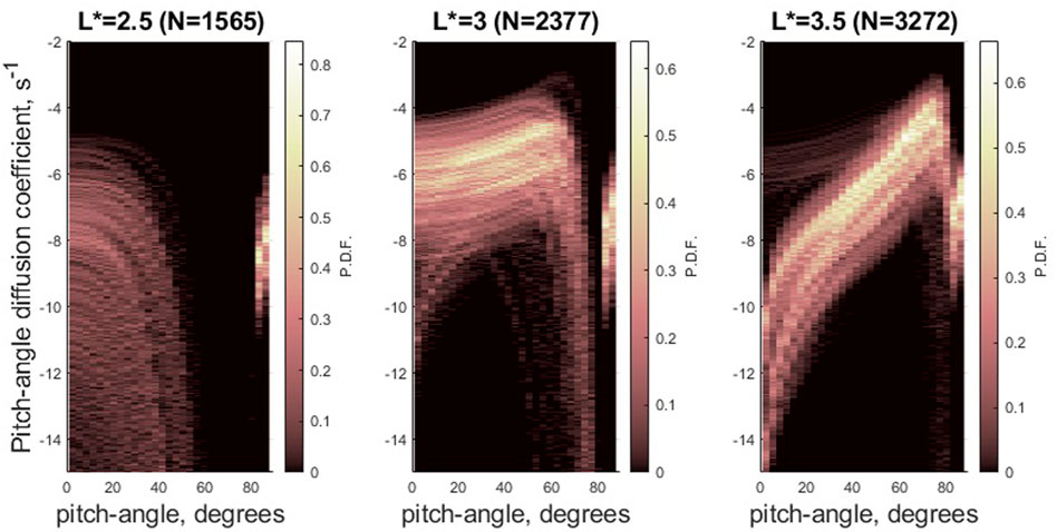
FIGURE 1. Probability distribution functions for Dαα(α) in each of the 3 L* bins used in this numerical study. The number of individual observation-specific Dαα(α) in each distribution N is indicated at the top of each panel. See (Watt et al., 2019) for choices made during construction of observation-specific Dαα.
We assign αLC in the numerical code to its equivalent value for a dipolar field line with L = L* for each bin. The observation bins are chosen to represent regions of the magnetosphere where plasmaspheric hiss is strong (Meredith et al., 2018), and the size of the bin is chosen to minimise potential radial or MLT variations in the distribution of Dαα(α). We therefore interpret the range of Dαα(α) in each bin as a result of temporal variation only. There are N > 1,000 individual Dαα(α) in each distribution, where N is indicated at the top of the Figure. It is important to reiterate (Watt et al., 2019; Watt et al., 2021) that both the shape and the strength of Dαα(α) varies as a result of the unique combination of δB2, ne and B0 used in its construction.
Each ensemble numerical experiment has 60 scenarios, i.e., 60 individual 30-day experiments are run with the same initial and boundary conditions, the same timescale of variability Δt, but different random selections of Dαα(α). Ensemble convergence for more than 60 scenarios in each ensemble is demonstrated in (Watt et al., 2021). The timescale of variability Δt is an important parameter in our numerical experiments. In each scenario in an ensemble of experiments, a time-series of Dαα(α, t) is constructed by randomly sampling the appropriate
In previous work (Watt et al., 2021), the small timescale chosen was Δt = 2 min, representing the typical length of time the spacecraft take to traverse the observation bin and over which there is often little variation in Dαα(α) [see Figure 2 of (Watt et al., 2021)]. The largest timescale chosen was Δt = 6 h, since it was clear from the orbital sampling of each observation bin that there is significant variation in Dαα(α) between each successive orbit. Our initial study indicated that there were significant differences in the ensemble results between Δt = 2 and Δt = 360 min. In this study, we investigate Δt = 2, 10, 30, 120, 240 and 360 min to determine how the results change with temporal scale.
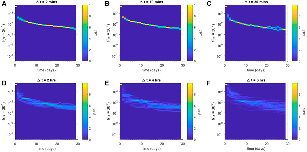
FIGURE 2. Ensemble results for numerical diffusion experiments using Dαα(L* = 2.5). Each panel shows a column-normalised probability distribution function for the phase space density f just outside the loss-cone αLC for (A) Δt = 2 min, (B) Δt = 10 min, (C) Δt = 30 min, (D) Δt = 2 h, (E) Δt = 4 h, and (F) Δt = 6 h. Note that each histogram is displayed using the same vertical binning, giving the histograms a pixelated appearance.
3 Results from numerical experiments
For each numerical experiment, we have 60 scenarios of f (α, t) at 1° resolution in α and 0.1 s resolution in time. To visualize one of the important aspects of the evolution of the ensembles, we choose a value of pitch-angle that is close to but greater than, αLC and plot the probability distribution function of the ensemble as a function of time. For L* = 2.5, we plot f (α = 13°), for L* = 3.0, we plot f (α = 10°) and for L* = 3.5, we plot f (α = 9°).
The results for the L* = 2.5 bin are shown in Figure 2, where Δt is (a) 2 min, (b), 10 min, (c) 30 min, (d) 120 min, (e) 240 min and (f) 360 min. Panel (a) shows that for the rapidly-varying diffusion coefficients, the ensemble exhibits very little variation from one scenario to another; the probability distribution function has a large peak and very little spread. The evolution of the peak of the distribution indicates a rapid initial drop as the loss-cone is evacuated, followed by a slower decline as pitch-angle scattering acts to smooth out the sharp gradient at the loss-cone. As Δt increases [moving from panels (a) to (f)], the ensemble results show much more spread. The probability distribution function exhibits increasing variation as Δt increases, even though the median ensemble behaviour is similar. Note that in each case, the median behaviour of the ensemble is similar to the behaviour of a numerical diffusion experiment using a diffusion coefficient averaged over the entire distribution of individual diffusion coefficients, Dαα,ave(α) = ⟨Dαα,i(α)⟩. We have chosen not to show this explicitly in individual panels of Figure 2 in order to highlight the narrowness of the distributions in panels (a) and (b), but a comparison can be made with Figure 4A of (Watt et al., 2021).
Figure 3 displays results from the numerical ensemble experiment using diffusion coefficients from the L* = 3 bin. In this case, the diffusion coefficients for E = 0.5 MeV tend to be much larger than those at L* = 2.5, and so the values of f (αLC) reach much lower values than in Figure 2. Similar trends exist as Δt is increased from 2 min to 360 min: for rapidly varying Dαα(α), the probability distribution function is strongly peaked with little spread. As Δt increases, the probability distribution function exhibits significant spread.
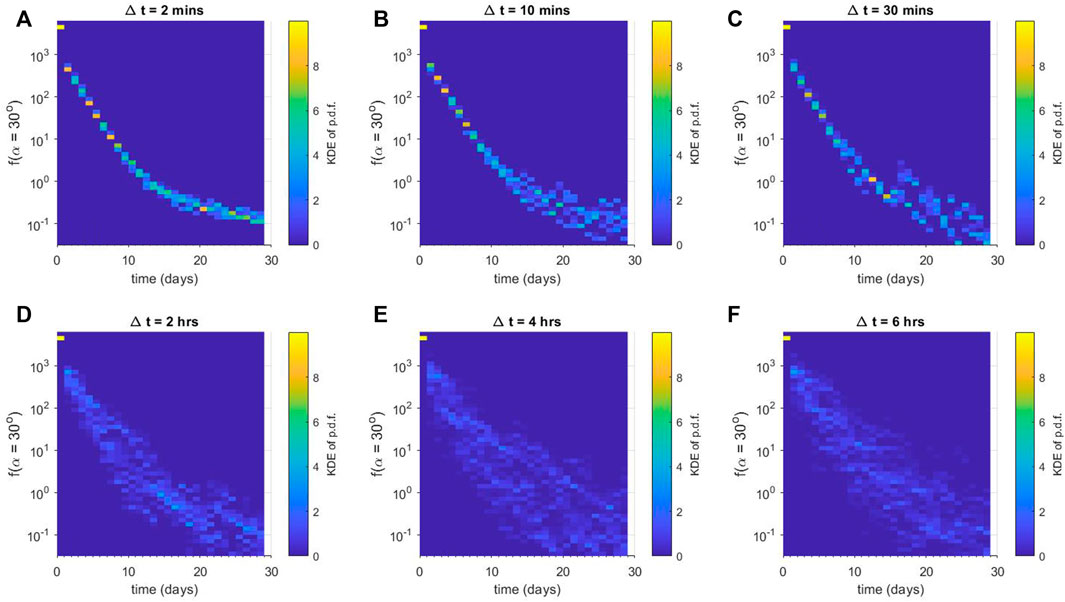
FIGURE 3. Ensemble results for numerical diffusion experiments using Dαα(L* = 3). Each panel shows a column-normalised probability distribution function for the phase space density f just outside the loss-cone αLC for (A) Δt = 2 min, (B) Δt = 10 min, (C) Δt = 30 min, (D) Δt = 2 h, (E) Δt = 4 h, and (F) Δt = 6 h. Note that each histogram is displayed using the same vertical binning, giving the histograms a pixelated appearance.
Finally, we demonstrate the results from the numerical ensemble experiment with L* = 3.5 in Figure 4. In this observation bin, the values of Dαα(α) for E = 0.5 MeV are in general much smaller than those seen at L* = 2.5 or L* = 3. As expected, for all values of Δt the ensembles indicate that f (αLC) remains at much higher levels than for other L* experiments. For small values of Δt shown in panels (a), (b) and (c), we again observe that the probability distribution function of f (αLC) is strongly peaked and exhibits very little spread. For panels (d), (e) and (f), we see a significant increase in spread of the probability distribution function. Additionally, these numerical experiments exhibit new behaviour that is not seen in Figures 2, 3. For the period 2 < t < 8 days in panel (d), and 2 < t < 10 days in panels (e) and (f), there appears to be two different sets of solutions in the ensemble. There is a strong peak at the initial value f (αLC) = 5 × 103 cm−2s−1sr−1keV−1 that gradually decreases with time, indicating that for many scenarios in the ensemble, very little diffusion has occurred. For a minority of scenarios in each ensemble, a lot more diffusion has occurred, as indicated by a much wider peak in the probability distribution function for f (αLC) = 1–4 × 103 cm−2s−1sr−1keV−1. The strong peak at the initial value of f (αLC) fades more slowly as Δt increases.
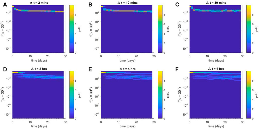
FIGURE 4. Ensemble results for numerical diffusion experiments using Dαα(L* = 3.5). Each panel shows a column-normalised probability distribution function for the phase space density f just outside the loss-cone αLC for (A) Δt = 2 min, (B) Δt = 10 min, (C) Δt = 30 min, (D) Δt = 2 h, (E) Δt = 4 h, and (F) Δt = 6 h. Note that each histogram is displayed using the same vertical binning, giving the histograms a pixelated appearance.
To compare directly between different Δt, we summarize the numerical experiment results in Figure 5. The top row [panels (a) to (c)] show the median of log10 [f (αLC)] for each ensemble as a function of time. The L* values are indicated at the top of the figure. The bottom row [panels (d) to (f)] show the interquartile range (IQR) of log10 [f (αLC)], again as a function of Δt and experiment time. To aid with interpretation of information in the bottom row, if IQR = 1 then there is an order of magnitude between the 25th percentile and the 75th percentile of the ensemble. Note that the median and IQR of log10 [f (αLC)] are used because the ensemble values of f (αLC) at each t are not normally-distributed (Watt et al., 2021).
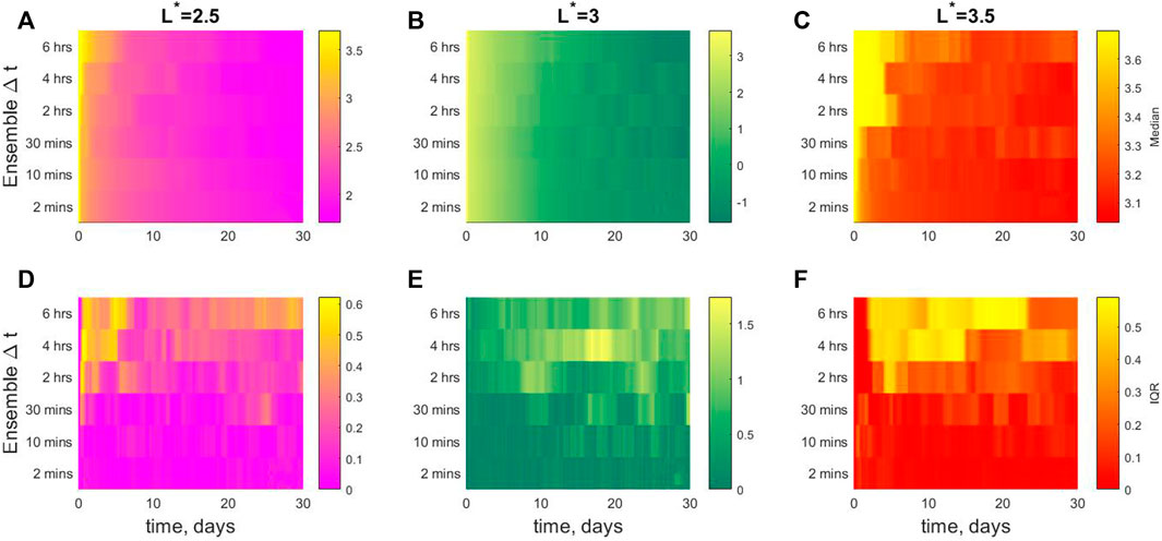
FIGURE 5. Summary figure for each L* set of experiments (A–C) median of log10 (f (αLC)) and (D–F) IQR of log10 (f (αLC)).
In general, Figure 5 shows that in each experiment the median value of log10 [f (αLC)] decreases more slowly as Δt increases, although for L* = 3.0 the difference in median behaviour is very small. The biggest difference between experiments comes when we consider the IQR; the ensemble results are much more variable as Δt increases. The IQR varies in time in each case, most notably so when Δt is large.
The value of log10f is important in modelling, as models are often interpreted and evaluated on a log scale. However, other physical quantities are important when judging the effects of temporal variability in the ensembles. The ensemble results also indicate large variability in the amount of loss-cone scattering due to plasmaspheric hiss. We calculated the percentage loss in each scenario by comparing the flux integrated over pitch-angle at the beginning of the experiment, and at the end of the experiment. Results are shown in Figure 6 where panels (a-c) show results from numerical experiments with Δt = 2 min, and panels (d-f) show results from experiments with Δt = 6 h. The amount of loss varies at each L* bin, as does the dependence of loss on Δt. At L* = 2.5, in the rapidly-varying experiments (i.e., low Δt), there is a total loss of flux of roughly 42% after 30 days in every scenario. However, for slowly-varying experiments (large Δt), the loss varies between 32% and 48%. At L* = 3.0, all scenarios, no matter the timescale, experience a loss of 85% in f over 30 days. Finally, for L* = 3.5, in the rapidly-varying experiments, all scenarios show a loss of 38%. However, for slowly-varying experiments, scenarios experience large differences in the amount of loss between 5% and 65%. The loss values are large across all experiments because the initial condition is a full loss cone that is immediately depleted. However, the variation in the amount of loss across the ensemble is due only to the differences in temporal variation in the diffusion coefficients between each scenario.
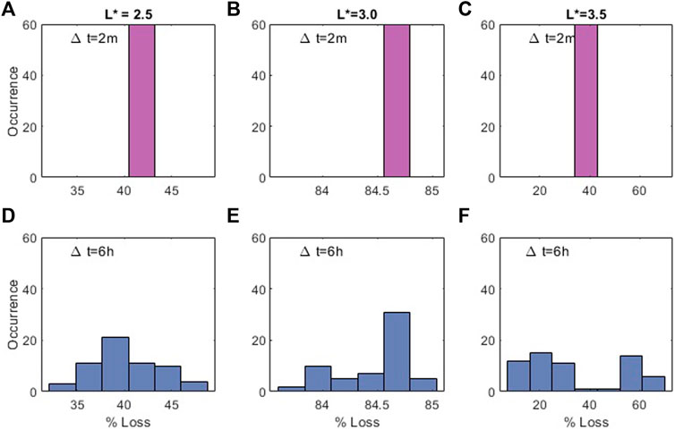
FIGURE 6. Histograms displaying percentage loss in each scenario from 6 different ensemble experiments: (A,D) use
4 Discussion
4.1 Diffusion coefficients modelled using quasi-linear theory
The quasi-linear theory of wave-particle interactions (Drummond and Pines, 1962; Kennel and Engelmann, 1966; Lyons et al., 1972; Lyons, 1974) yields diffusion coefficients Di,j such that microscopic wave-particle interactions may be included in numerical models with time and length scales that are much longer than those of the waves themselves. To construct models of diffusion coefficients, it is necessary to use observations or models of magnetospheric magnetic field, number density, and composition in addition to information about wave intensity and how it varies in space, frequency and wavenormal angle. We discuss here the implications of our numerical results for the accurate modelling of quasi-linear diffusion coefficients using observations from in-situ spacecraft.
We have modelled our diffusion coefficients using a statistical distribution of observation-specific (Watt et al., 2019; Ross et al., 2020) values. The free parameter in our numerical study is the temporal scale of variation Δt. Our results indicate that when used in ensembles of Fokker-Planck models, temporal variation of quasi-linear diffusion coefficients with timescales greater than 30 min yields significant uncertainty in the model results. For timescales of variation less than 30 min, an average of the observation-specific diffusion coefficients is a reasonable approximation to the ensemble result (Watt et al., 2021). Recent work (Zhang et al., 2021a) indicates that observed timescales for plasmaspheric hiss patches are typically less than 10 min, and so plasmaspheric hiss activity would appear to vary sufficiently rapidly that averaging observation-specific diffusion coefficients should be appropriate. We discuss timescales relative to drift-averaging in Section 4.3 below.
Quasi-linear diffusion coefficients must be calculated on timescales that are long compared to the wave period
Many models of Di,j are constructed from long-term statistical studies of wave activity in the magnetosphere. To connect observations to the Di,j, a grid is often constructed in real space on which to collect observations that are then statistically averaged. In-situ observations relative to that grid are collated and averaged to provide averaged wave amplitudes (Tu et al., 2013; Sicard-Piet et al., 2014; Li et al., 2015; Ma et al., 2017; Meredith et al., 2018; Zhu et al., 2019; Green et al., 2020; Meredith et al., 2020), averaged frequency distributions (Li et al., 2016; Zhu et al., 2019) or averaged wavenormal angle distributions (Ni et al., 2013). The averaged properties are then combined with models of the magnetic field and number density to form diffusion coefficient models (Horne et al., 2013; Wang et al., 2017; Ma et al., 2018). In each case, observations are averaged over many months, sometimes years or decades (Watt et al., 2017; Watt et al., 2019). During these long time periods, all of the inputs are highly variable (Watt et al., 2019). We therefore recommend that where observations are used to constrain models of quasi-linear diffusion coefficients:
• Di,j should be calculated using co-located and simultaneous measurements based upon a grid in e.g. magnetic local time and L*. Spacecraft such as the NASA Van Allen probes travel through such a grid rapidly enough that observations are quite similar within grid cells [see e.g., (Watt et al., 2019)], and so observations from a single pass through the grid should be used to construct each observation-specific diffusion coefficient.
• Statistical models should then be constructed from those observation-specific values [see e.g., (Ross et al., 2020)]
• The natural timescales of variation for diffusion due to each wave mode should be studied and quantified
• Where timescales of variation are sufficiently short (in the case of plasmaspheric hiss, less than around 30 min), averaged models can then be constructed from averages of the observation-specific values.
Note that although we focus only on the pitch-angle scattering coefficient Dαα due to plasmaspheric hiss in this work, the consequences of our results should hold for diffusion coefficients in energy and the cross-terms (Albert et al., 2009), as well as for diffusion coefficients describing wave-particle interactions with other wave modes.
4.2 Temporal scales of variability leads to different levels of uncertainty in model results
It is important to carefully interpret the ensemble results. The median of the ensemble provides an indication of the general trend when a collection of numerical scenarios are grouped together. No single ensemble scenario resembles the median evolution; each individual scenario experiences rare big changes when large values of diffusion coefficients are chosen from the distribution, with very little change at other times when only small values of diffusion coefficients are experienced [see Figure 3 of (Watt et al., 2021) for an example]. The IQR is a measure of the variability of each numerical ensemble. We reiterate from our initial study (Watt et al., 2021) that the time-integrated diffusion in all experiments at the same L* is the same, the only difference in each case is the value of Δt.
The IQR in each ensemble experiment depends both on Δt and the average strength of the diffusion coefficients in the distribution
In contrast, large IQR values where Δt is large, or average diffusion rates are large, indicate significant amounts of uncertainty in the outcome of the ensemble numerical experiments. For example, the IQR is more than an order of magnitude in most experiments using
The numerical experiments reported here only consider resonant quasilinear diffusion coefficients [e.g., (Lyons et al., 1972; Lyons, 1974)]. However, non-resonant wave-particle interactions [e.g., (Zhao et al., 2022)], although usually much weaker, also depend upon wave amplitudes. For the most intense waves, the nonresonant interaction could be as large as the resonant interaction during typical periods. We advocate more research in this important area, towards possible inclusion in large-scale radiation belt models.
Uncertainty in the model results shown in Figures 2–4 provide bounds and other statistical information regarding potential solutions to the diffusion equation under idealized circumstances. In some cases, these bounds are very wide. Over a 30-day period, with no other influences on the evolution of the numerical experiment other than the changing diffusion coefficients (e.g., no sources of phase space density either due to radial or energy diffusion), the uncertainty in the experiments changes in time (see also Figure 5). This is especially marked for large Δt. Large uncertainties in the ensemble solutions can arise due to the changes in the shape of Dαα(α) as well as in its strength. The range of α over which Dαα is large can change with plasma to gyrofrequency ratio (Horne and Thorne, 2003; Glauert and Horne, 2005; Watt et al., 2019). For some values of this ratio, the range of large Dαα can momentarily extend to large α, and act like a temporary source of plasma to be diffused to low α. These effects are associated with periods of large and varying uncertainty in the ensemble numerical experiments.
When we envisage using stochastic parameterizations of Dij in full 3D radiation belt diffusion models, the consequences of large variability may be compounded. For example, the uncertainties in the amount of loss (Figure 6) can be very large. There is a complicated relationship between the size and shape of the diffusion coefficients, and the resulting uncertainty. In a full 3D diffusion model with diffusion across pitch-angle, energy and L* space, it is likely that the interplay of uncertainty in diffusion in three dimensions, as well as uncertainty due to variable physical sources included through boundary conditions in L* and energy space, will result in significantly more uncertainty as models progress. We argue that the results presented here prompt us to seek ways to reduce the uncertainty in the diffusion coefficients used in radiation belt models. Reducing uncertainty is not just about reducing error bars of a model, reducing uncertainty reduces the number of potential paths a model might take through the potential solutions of phase space density in (L*, E, α) space. Identifying and reducing uncertainty in diffusion coefficient descriptions (Bentley et al., 2019; Watt et al., 2019), boundary conditions, and even the magnetic field models used in coordinate transforms (Loridan et al., 2019; Thompson et al., 2021) will allow us to use models 1) to correctly attribute a change in radiation belt evolution to a particular physical process (Mann et al., 2016; Shprits et al., 2018), 2) to identify a realistic range of radiation belt responses to geomagnetic disturbances or 3) as an effective operational forecast tool.
Where Δt is large, or average diffusion rates are large, uncertainty in model behaviour could be reduced by minimizing the variability in the distribution of diffusion coefficients (Thompson et al., 2020). Reduction of variability can be achieved through parameterization (Bentley et al., 2019), i.e., where diffusion coefficients are binned according to parameters that control their behaviour. Parameterizations are widely used to construct wave amplitude maps (Horne et al., 2013; Glauert et al., 2014; Bentley et al., 2018; Bentley et al., 2020; Meredith et al., 2020; Aryan et al., 2021), and could be used to construct models of diffusion coefficients equally as effectively (Watt et al., 2019; Ross et al., 2020).
4.3 Temporal variability and drift-averaging
Our numerical experiments indicate that there are some circumstances where averaging is appropriate. It is therefore important to determine whether this is true for drift-averaging. It is therefore important to determine whether Recent work (Zhang et al., 2021a) has characterised the temporal and spatial scale sizes of patches of plasmaspheric hiss in the inner magnetosphere. Using both NASA Van Allen Probe spacecraft (Mauk et al., 2013), integrated wave power from the Wave Form Receiver in the Electric and Magnetic Field Instrument Suite and Integrated Science [EMFISIS (Kletzing et al., 2013)] was cross-correlated. The varying separation of the two Van Allen Probes as they travel on similar orbits allows good estimates of both temporal and spatial correlations. Spatial correlations are estimated by correlating the time series of integrated wave power from each satellite with no lag. Zhang et al. (2021a) demonstrated that correlations were higher when the spacecraft were closely separated in space less than
Although diffusion coefficients depend both on wave amplitude and local parameters such as number density and magnetic field strength, here we will use the results of Zhang et al. (2021a) to consider constraints on the temporal and spatial scales of the plasmaspheric hiss itself. Future investigations should be performed to incorporate the spatial and temporal variability of the number density in the inner magnetosphere, as it is a key parameter in the calculation of diffusion coefficients (see Section 4.4).
In Figure 7, we collect data from the Zhang et al. (2021a) study where both Van Allen Probes have L* < 4 to coincide with our observation bins at L* = 2.5, 3.0 and 3.5. Figure 7A shows a histogram of temporal lags when the correlation coefficient of the two spacecraft observations R2 > 0.5. The high correlation is used as identification of coherent spatial patches of plasmaspheric hiss activity. The corresponding temporal lags indicate that patches last for a few minutes with an observed maximum of around 25 min. Figure 7B shows the amplitude ratio for the same patches indicating that when the correlation is high, the amplitudes of the patches observed by each spacecraft are similar. If we assume that the patches are not moving in space, then we can interpret the temporal lags as the temporal scale of the patches. When we compare to the results of the numerical experiments, the hiss patch timescale (
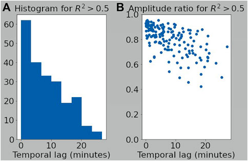
FIGURE 7. (A) Histogram of temporal lags between spacecraft that yield correlations with R2 > 0.5 for whistler-mode wave power. (B) Amplitude ratio of whistler-mode waves measured by each spacecraft for temporal lags shown in histogram. Subset of correlation data where Van Allen Probes A and B both have L* < 4 taken from Zhang et al. (2021a).
It is important to note that when constructing a diffusion coefficient for a high-energy electron (e.g., with E = 0.5 MeV), we must also consider its experience as it drifts around the Earth under the influence of gradient and curvature drifts. Some of the “temporal” changes in wave-particle interactions experienced by the drifting electron arise due to its rapid transit of spatially coherent patches of plasmaspheric hiss, and so we must also consider the spatial size of these patches. Figure 8 shows a subset of data with L* < 4 from the Zhang et al. (2021a), study, but this time looking at spatial correlations. Figure 8A shows a histogram of spatial separations when the correlation coefficient of the two spacecraft observations R2 > 0.5. Note that events in this study are chosen such that the spacecraft separation is
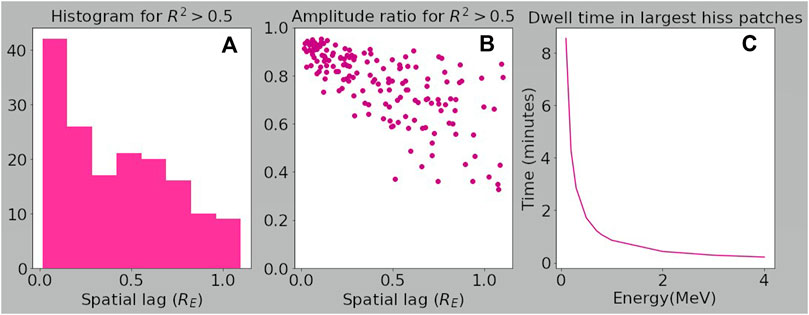
FIGURE 8. (A) Histogram of spatial lags between spacecraft that yield correlations with R2 > 0.5 for whistler-mode wave power. (B) Amplitude ratio of whistler-mode waves measured by each spacecraft for spatial lags shown in histogram. (C) Estimated dwell time in largest observed whistler-mode wave patches as a function of energy. Subset of correlation data where Van Allen Probes A and B both have L* < 4 taken from Zhang et al. (2021a).
We consider the largest plasmaspheric hiss patches identified in the Zhang et al. (2021a), study (with the caveat that this largest value is self-imposed), and estimate how long it would take electrons of different energies to gradient-curvature drift through the patches at L* = 3. Assuming the magnetic field is essentially dipolar, and that electrons have 90° pitch-angles, dwell times in hiss patches with scale sizes of 1RE are shown in Figure 8C. For the example energy considered throughout this paper (E = 0.5 MeV), dwell times are less than 3 min. So when we consider the apparent timescales of wave patches, as experienced by a drifting high-energy electron at L* = 3, these also correspond to the smallest values of Δt < 10 min used in the numerical experiments, which again show low values of uncertainty.
Given the numerical experiment results reported here, our analysis of the temporal and spatial scale sizes of patches of plasmaspheric hiss indicate that averaging of diffusion coefficients in the azimuthal direction would provide reasonably accurate determinations of drift-averaged diffusion coefficients as experienced by high-energy electrons in the outer radiation belt. In all of our numerical experiments where we model the variability of wave-particle interactions using small timescales similar to those experienced by an electron as it drifts through a plasmaspheric hiss patch, ensemble scenarios are very similar, and the evolution of the model closely follows that of a model performed with an arithmetic average of the diffusion coefficients. Even when the underlying distribution of diffusion coefficients varies over many orders of magnetidue (see Figure 1), if the timescales of varation are rapid enough, ensembles produce very similar results that tend to the same behaviour as experiments run with averaged values (Watt et al., 2021). Note that averaging is less accurate and leads to more uncertainty as the average value of the diffusion coefficients increases.
We therefore suggest that it is important to perform an analysis of the temporal variation of drift-averaged diffusion coefficients in the magnetosphere. For plasmaspheric hiss, this could be achieved with probabilistic models of the evolution and spatial structure of wave patches, using distributions of observed wave amplitudes (Watt et al., 2019) and information about their spatial and temporal scales (Zhang et al., 2021a) as well as their distribution in L* and relative to the plasmapause (Malaspina et al., 2016).
For other magnetospheric waves, such as whistler-mode chorus, it will be necessary to study the effects of averaging the wave-particle interactions over the bursty structure of chorus elements (Li et al., 2012), and over the temporal extent of chorus patches (Zhang et al., 2021b). For chorus, temporal variation is often very fast, again suggesting that arithmetic averages might be reasonable approximations, especially for constructing drift-averages. However, we reiterate the importance of determining how the drift-averaged diffusion coefficients vary in time, given what we know about chorus wave behaviour in time and space (Aryan et al., 2016; Agapitov et al., 2018; Shen et al., 2019; Zhang et al., 2021b). The temporal variation of drift-averaged quasilinear diffusion coefficients is currently a key unknown in our modelling efforts.
Note that in the 3 L* cases we have studied, the average value of the diffusion coefficient at αLC is
4.4 The importance of number density in wave-particle interactions
We turn finally to the ensemble experimental results that display some bifurcation for large Δt, namely those for L* = 3.5 (see Figure 4). These ensembles are different from others at early times: most of the ensemble members show very little diffuson, whereas a minority display much more. To understand these differences, we analyse the
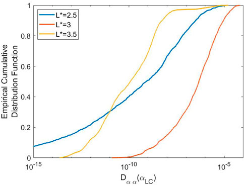
FIGURE 9. Cumulative distribution functions of the
The existence of multiple distributions of diffusion coefficients at L* = 3.5 is a possible explanation for the behaviour of the ensemble of numerical solutions of f (αLC) in Figure 4. Let’s consider the experiments with large Δt first. For early times in the ensemble (
The unexpectedly large values of Dαα(α) in the upper
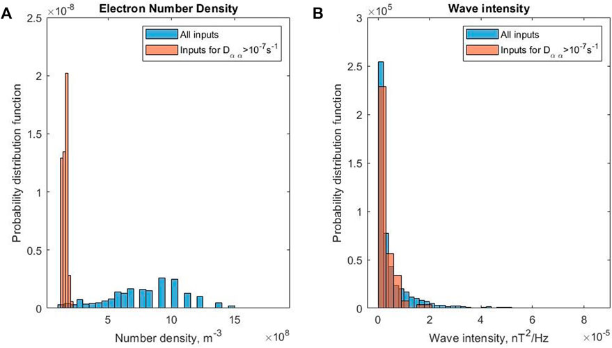
FIGURE 10. Probability distribution functions of (A) electron number density and (B) wave intensity inputs for calculation of Dαα(α) at L* = 3.5. Blue bars show inputs for the entire collection of Dαα(α), orange bars indicate inputs for Dαα(αLC) > 10–7 s−1.
Figure 10A demonstrates that the number density inputs to the diffusion coefficient calculations for particularly high values of Dαα(αLC) are consistently the lowest values of the overall distribution of number density inputs. In our original diffusion coefficient study (Watt et al., 2019), we applied the Sheeley et al. (2001) number density criterion to identify observations inside and outside the plasmasphere. Although these measurements correspond to values close to that criterion, they are identified as inside the plasmasphere. Figure 10B shows the distribution of wave intensity for Dαα(αLC) > 10–7 s−1 (orange) compared to all inputs at L* = 3.5 (blue) For the wave intensity parameter, there is little difference in the distributions between the particularly large Dαα(αLC) and all the Dαα(αLC). We suggest that the origin of the two distributions in Dαα is mostly related to the number density. This feature is only seen in the largest L* bin used in the study, most likely because the other two are too far away from the more dynamic density region closer to the plasmapause.
We interpret these results to indicate the key importance of electron number density in the efficacy of scattering due to plasmaspheric hiss. The plasmapause is not always a sharp boundary and exhibits a lot of spatial and temporal structure (Moldwin et al., 1994; Moldwin et al., 2002), yet rare periods of relatively low density (that are likely near the plasmapause) are very important for wave-particle interactions with hiss as they can result in much higher than usual diffusion coefficients. The temporal and spatial variability for density may be different than that for wave amplitude which would complicate our suggested study of the temporal variability of drift-averaged diffusion coefficients. However, our study adds weight to the increasing evidence for the importance of number density in models of wave diffusion coefficients in Earth’s radiation belts (Ripoll et al., 2016; Ripoll et al., 2020a; Ripoll et al., 2020b; Allison et al., 2021).
5 Conclusion
We use ensemble numerical experiments with diffusion coefficient models that are driven by individual Van Allen Probe observations in order to study the pitch-angle diffusion due to plasmaspheric hiss in Earth’s magnetosphere. We demonstrate that ensemble solutions of the Fokker-Planck equation depend both upon the timescale of variability (varied between minutes and hours), and the shape of the distribution of diffusion coefficients. The median ensemble solutions vary slightly with timescale, but the inter-quartile range (or variance) of the ensemble solutions depends both upon the timescale and the strength of the diffusion coefficients; longer timescales, and larger average diffusion coefficients result in larger variance.
We use observed time and length scales of plasmaspheric hiss patches to identify suitable methods to construct appropriate drift-averaged diffusion coefficients for high-energy drifting electrons. Arithmetic averaging of observation-specific diffusion coefficients is appropriate in many cases due to the small temporal and spatial scales of hiss patches, although arithmetic drift-averaging will become less accurate as the size of the diffusion coefficients increases. We argue that arithmetic averaging of observed inputs (e.g., wave amplitude, wave frequency spectrum, number density or background magnetic field strength) prior to constructing diffusion coefficients does not yield appropriate averaged values of the diffusion coefficient because there is a maximum useful averaging timescale that for many missions is shorter than the orbital period.
The distribution of observation-specific diffusion coefficients is found to vary with L*. In two of the three chosen bins, the distribution of diffusion coefficients is a single probability distribution. In the remaining chosen location, which is at larger L*, the probability distribution exhibits two different components, where rare but large values of the diffusion coefficient occur during periods of low number density. We argue that it is of vital importance to include accurate cold plasma models to radiation belt diffusion codes to improve the description of wave-particle interactions, especially during times when they are most effective.
Our results, along with others (Thompson et al., 2020; Watt et al., 2021), indicate the importance of understanding timescales of variation of wave-particle interactions throughout the outer radiation belt. Once these timescales are understood, numerical experiments similar to those reported here can be used to indicate where further parameterisation is necessary in order to reduce the uncertainty in our models. Due to the limited temporal and spatial sampling by spacecraft of localised waves and plasma properties in the outer radiation belt, some kind of model will always be required to monitor the evolution of drift-averaged quasilinear diffusion coefficients in Earth’s magnetosphere. In this paper we have endeavoured to motivate further important work in this area.
Data availability statement
The datasets presented in this study can be found in online repositories. The names of the repository/repositories and accession number(s) can be found below: https://emfisis.physics.uiowa.edu/data/index; https://doi.org/10.17864/1947.212, Ensemble experiment data can be found at https://doi.org/10.25398/rd.northumbria.2126623.
Author contributions
CW and HA conceived the numerical experiments, in consultation with SB and RT. HA wrote numerical software and performed the numerical experiments. CW analyzed and visualized the results of the numerical experiments, and constructed all Figures. NM curated the Van Allen Probe data necessary to construct the observation-specific diffusion coefficients. SG provided the PADIE software necessary to construct the diffusion coefficients and advised on its use. SZ contributed key analysis of Van Allen Probe data enabling CW to construct Figures 7, 8. DR and SK wrote software necessary for discussion in Section 4.3. IR, OA, SG, JR, RH, NM, and KM provided interpretation of the ensemble numerical experiment results and discussion points. CW wrote the first draft of the manuscript. All authors contributed to editing the manuscript before submission.
Funding
This work was enabled by collaborations supported by the Natural Environment Research Council (NERC) Highlight Topic consortium “Rad-Sat,” and the Space Weather Instrumentation, Measurement, Modelling and Risk (SWIMMR) Strategic Priorities Fund consortium “Sat-Risk.” Individual grant numbers are noted below. CW is supported by Science and Technology Facilities Council (STFC) grant ST/W000369/1 and Natural Environment Research Council (NERC) grants NE/P017274/1 (Rad-Sat) and NE/V002759/2 (Sat-Risk). HA is supported by an Alexander von Humboldt Postdoctoral Research Fellowship. IR acknowledges support from STFC grant ST/V006320/1 and NERC grants NE/P017185/1 (Rad-Sat) and NE/V002554/2 (Sat-Risk). NM, RH, SG, and JR would like to acknowledge financial support from the NERC Highlight Topic grant NE/P01738X/1 (Rad-Sat) and the NERC grants NE/V00249X/1 (Sat-Risk) and NE/R016038/1. OA acknowledges financial support from the University of Exeter and from the United Kingdom Natural Environment Research Council (NERC) Independent Research Fellowship NE/V013963/1, as well as NE/P017274/1 (Rad-Sat).
Acknowledgments
The authors acknowledge the NASA Van Allen Probes EMFISIS team led by Craig Kletzing at the University of Iowa for the successful build and operation of the high-quality science instruments onboard both probes. The CDAWeb team at GSFC/SPDF are also gratefully acknowledged.
Conflict of interest
The authors declare that the research was conducted in the absence of any commercial or financial relationships that could be construed as a potential conflict of interest.
Publisher’s note
All claims expressed in this article are solely those of the authors and do not necessarily represent those of their affiliated organizations, or those of the publisher, the editors and the reviewers. Any product that may be evaluated in this article, or claim that may be made by its manufacturer, is not guaranteed or endorsed by the publisher.
References
Agapitov, O., Mourenas, D., Artemyev, A., Mozer, F. S., Bonnell, J. W., Angelopoulos, V., et al. (2018). Spatial extent and temporal correlation of chorus and hiss: Statistical results from multipoint THEMIS observations. JGR. Space Phys. 123, 8317–8330. doi:10.1029/2018JA025725
Albert, J. M., Meredith, N. P., and Horne, R. B. (2009). Three-dimensional diffusion simulation of outer radiation belt electrons during the 9 October 1990 magnetic storm. J. Geophys. Res. 114. doi:10.1029/2009JA014336
Allanson, O., Elsden, T., Watt, C., and Neukirch, T. (2022). Weak turbulence and quasilinear diffusion for relativistic wave-particle interactions via a markov approach. Front. Astron. Space Sci. 8. doi:10.3389/fspas.2021.805699
Allanson, O., Watt, C. E. J., Ratcliffe, H., Allison, H. J., Meredith, N. P., Bentley, S. N., et al. (2020). Particle-in-cell experiments examine electron diffusion by whistler-mode waves: 2. Quasi-linear and nonlinear dynamics. J. Geophys. Res. Space Phys. 125, e2020JA027949. doi:10.1029/2020JA027949
Allanson, O., Watt, C. E. J., Ratcliffe, H., Meredith, N. P., Allison, H. J., Bentley, S. N., et al. (2019). Particle-in-cell experiments examine electron diffusion by whistler-mode waves: 1. Benchmarking with a cold plasma. J. Geophys. Res. Space Phys. 124, 8893–8912. doi:10.1029/2019JA027088
Allison, H. J., and Shprits, Y. Y. (2020). Local heating of radiation belt electrons to ultra-relativistic energies. Nat. Commun. 11, 4533. doi:10.1038/s41467-020-18053-z
Allison, H. J., Shprits, Y. Y., Zhelavskaya, I. S., Wang, D., and Smirnov, A. G. (2021). Gyroresonant wave-particle interactions with chorus waves during extreme depletions of plasma density in the van allen radiation belts. Sci. Adv. 7, eabc0380. doi:10.1126/sciadv.abc0380
Anderson, B. J., Erlandson, R. E., and Zanetti, L. J. (1992). A statistical study of pc 1–2 magnetic pulsations in the equatorial magnetosphere: 1. Equatorial occurrence distributions. J. Geophys. Res. 97, 3075–3088. doi:10.1029/91JA02706
Aryan, H., Bortnik, J., Meredith, N. P., Horne, R. B., Sibeck, D. G., and Balikhin, M. A. (2021). Multi-parameter chorus and plasmaspheric hiss wave models. JGR. Space Phys. 126, e2020JA028403. doi:10.1029/2020JA028403
Aryan, H., Sibeck, D., Balikhin, M., Agapitov, O., and Kletzing, C. (2016). Observation of chorus waves by the van allen probes: Dependence on solar wind parameters and scale size. J. Geophys. Res. Space Phys. 121, 7608–7621. doi:10.1002/2016JA022775
Bentley, S. N., Stout, J. R., Bloch, T. E., and Watt, C. E. J. (2020). Random forest model of ultralow-frequency magnetospheric wave power. Earth Space Sci. 7, e2020EA001274. doi:10.1029/2020EA001274
Bentley, S. N., Watt, C. E. J., Owens, M. J., and Rae, I. J. (2018). Ulf wave activity in the magnetosphere: Resolving solar wind interdependencies to identify driving mechanisms. J. Geophys. Res. Space Phys. 123, 2745–2771. doi:10.1002/2017JA024740
Bentley, S. N., Watt, C. E. J., Rae, I. J., Owens, M. J., Murphy, K., Lockwood, M., et al. (2019). Capturing uncertainty in magnetospheric ultralow frequency wave models. Space weather. 17, 599–618. doi:10.1029/2018SW002102
Cervantes, S., Shprits, Y. Y., Aseev, N. A., Drozdov, A. Y., Castillo, A., and Stolle, C. (2020). Identifying radiation belt electron source and loss processes by assimilating spacecraft data in a three-dimensional diffusion model. JGR. Space Phys. 125, e2019JA027514. doi:10.1029/2019JA027514
Drummond, W., and Pines, D. (1962). Nonlinear stability of plasma oscillations. Nucl. Fusion Suppl. Pt 2, 465.
Fei, Y., Chan, A. A., Elkington, S. R., and Wiltberger, M. J. (2006). Radial diffusion and mhd particle simulations of relativistic electron transport by ulf waves in the september 1998 storm. J. Geophys. Res. 111, A12209. doi:10.1029/2005JA011211
Glauert, S. A., and Horne, R. B. (2005). Calculation of pitch angle and energy diffusion coefficients with the padie code. J. Geophys. Res. 110. doi:10.1029/2004JA010851
Glauert, S. A., Horne, R. B., and Meredith, N. P. (2014). Three-dimensional electron radiation belt simulations using the BAS Radiation Belt Model with new diffusion models for chorus, plasmaspheric hiss, and lightning-generated whistlers. J. Geophys. Res. Space Phys. 119, 268–289. doi:10.1002/2013JA019281
Green, A., Li, W., Ma, Q., Shen, X. C., Bortnik, J., and Hospodarsky, G. B. (2020). Properties of lightning generated whistlers based on van allen probes observations and their global effects on radiation belt electron loss. Geophys. Res. Lett. 47, e2020GL089584. doi:10.1029/2020GL089584
Halford, A. J., Fraser, B. J., and Morley, S. K. (2010). Emic wave activity during geomagnetic storm and nonstorm periods: Crres results. J. Geophys. Res. 115. doi:10.1029/2010JA015716
Hikishima, M., and Omura, Y. (2012). Particle simulations of whistler-mode rising-tone emissions triggered by waves with different amplitudes. J. Geophys. Res. 117. doi:10.1029/2011JA017428
Horne, R. B., Kersten, T., Glauert, S. A., Meredith, N. P., Boscher, D., Sicard-Piet, A., et al. (2013). A new diffusion matrix for whistler mode chorus waves. J. Geophys. Res. Space Phys. 118, 6302–6318. doi:10.1002/jgra.50594
Horne, R. B., and Thorne, R. M. (2003). Relativistic electron acceleration and precipitation during resonant interactions with whistler-mode chorus. Geophys. Res. Lett. 30. doi:10.1029/2003GL016973
Horne, R. B., Thorne, R. M., Shprits, Y. Y., Meredith, N. M., Glauert, S. A., Smith, A. J., et al. (2005). Wave acceleration of electrons in the Van Allen radiation belts. Nature 437, 227–230. doi:10.1038/nature03939
Kennel, C. F., and Engelmann, F. (1966). Velocity space diffusion from weak plasma turbulence in a magnetic field. Phys. Fluids 9, 2377–2388. doi:10.1063/1.1761629
Kim, K. C., and Shprits, Y. (2019). Statistical analysis of hiss waves in plasmaspheric plumes using van allen probe observations. J. Geophys. Res. Space Phys. 124, 1904–1915. doi:10.1029/2018JA026458
Kim, K. C., Shprits, Y., and Wang, D. (2020). Quantifying the effect of plasmaspheric hiss on the electron loss from the slot region. J. Geophys. Res. Space Phys. 125, e2019JA027555. doi:10.1029/2019JA027555
Kletzing, C. A., Kurth, W. S., Acuna, M., MacDowall, R. J., Torbert, R. B., Averkamp, T., et al. (2013). The electric and magnetic field instrument suite and integrated science (emfisis) on rbsp. Space Sci. Rev. 179, 127–181. doi:10.1007/s11214-013-9993-6
Lemons, D. S. (2012). Pitch angle scattering of relativistic electrons from stationary magnetic waves: Continuous markov process and quasilinear theory. Phys. Plasmas 19, 012306. doi:10.1063/1.3676156
Li, J., Bortnik, J., An, X., Li, W., Angelopoulos, V., Thorne, R. M., et al. (2019). Origin of two-band chorus in the radiation belt of Earth. Nat. Commun. 10, 4672. doi:10.1038/s41467-019-12561-3
Li, W., Ma, Q., Thorne, R. M., Bortnik, J., Kletzing, C. A., Kurth, W. S., et al. (2015). Statistical properties of plasmaspheric hiss derived from Van Allen Probes data and their effects on radiation belt electron dynamics. JGR. Space Phys. 120, 3393–3405. doi:10.1002/2015JA021048
Li, W., Ma, Q., Thorne, R. M., Bortnik, J., Zhang, X. J., Li, J., et al. (2016). Radiation belt electron acceleration during the 17 march 2015 geomagnetic storm: Observations and simulations. JGR. Space Phys. 121, 5520–5536. doi:10.1002/2016JA022400
Li, W., Thorne, R. M., Angelopoulos, V., Bortnik, J., Cully, C. M., Ni, B., et al. (2009). Global distribution of whistler-mode chorus waves observed on the themis spacecraft. Geophys. Res. Lett. 36, L09104. doi:10.1029/2009GL037595
Li, W., Thorne, R. M., Bortnik, J., Tao, X., and Angelopoulos, V. (2012). Characteristics of hiss-like and discrete whistler-mode emissions. Geophys. Res. Lett. 39. doi:10.1029/2012GL053206
Liu, K., Winske, D., Gary, S. P., and Reeves, G. D. (2012). Relativistic electron scattering by large amplitude electromagnetic ion cyclotron waves: The role of phase bunching and trapping. J. Geophys. Res. 117. doi:10.1029/2011JA017476
Loridan, V., Ripoll, J. F., Tu, W., and Scott Cunningham, G. (2019). On the use of different magnetic field models for simulating the dynamics of the outer radiation belt electrons during the october 1990 storm. J. Geophys. Res. Space Phys. 124, 6453–6486. doi:10.1029/2018JA026392
Lyons, L. R. (1974). Pitch angle and energy diffusion coefficients from resonant interactions with ion–cyclotron and whistler waves. J. Plasma Phys. 12, 417–432. doi:10.1017/S002237780002537X
Lyons, L. R., Thorne, R. M., and Kennel, C. F. (1972). Pitch-angle diffusion of radiation belt electrons within the plasmasphere. J. Geophys. Res. 77, 3455–3474. doi:10.1029/JA077i019p03455
Ma, Q., Li, W., Bortnik, J., Thorne, R. M., Chu, X., Ozeke, L. G., et al. (2018). Quantitative evaluation of radial diffusion and local acceleration processes during gem challenge events. JGR. Space Phys. 123, 1938–1952. doi:10.1002/2017JA025114
Ma, Q., Mourenas, D., Li, W., Artemyev, A., and Thorne, R. M. (2017). Vlf waves from ground-based transmitters observed by the van allen probes: Statistical model and effects on plasmaspheric electrons. Geophys. Res. Lett. 44, 6483–6491. doi:10.1002/2017GL073885
Malaspina, D. M., Jaynes, A. N., Boulé, C., Bortnik, J., Thaller, S. A., Ergun, R. E., et al. (2016). The distribution of plasmaspheric hiss wave power with respect to plasmapause location. Geophys. Res. Lett. 43, 7878–7886. doi:10.1002/2016GL069982
Mann, I. R., Ozeke, L. G., Murphy, K. R., Claudepierre, S. G., Turner, D. L., Baker, D. N., et al. (2016). Explaining the dynamics of the ultra-relativistic third Van Allen radiation belt. Nat. Phys. 12, 978–983. doi:10.1038/nphys3799
Mauk, B. H., Fox, N. J., Kanekal, S. G., Kessel, R. L., Sibeck, D. G., and Ukhorskiy, A. (2013). Science objectives and rationale for the radiation belt storm probes mission. Space Sci. Rev. 179, 3–27. doi:10.1007/s11214-012-9908-y
Meredith, N. P., Horne, R. B., Clilverd, M. A., and Ross, J. P. J. (2019). An investigation of vlf transmitter wave power in the inner radiation belt and slot region. JGR. Space Phys. 124, 5246–5259. doi:10.1029/2019JA026715
Meredith, N. P., Horne, R. B., Kersten, T., Fraser, B. J., and Grew, R. S. (2014). Global morphology and spectral properties of emic waves derived from crres observations. J. Geophys. Res. Space Phys. 119, 5328–5342. doi:10.1002/2014JA020064
Meredith, N. P., Horne, R. B., Kersten, T., Li, W., Bortnik, J., Sicard, A., et al. (2018). Global model of plasmaspheric hiss from multiple satellite observations. JGR. Space Phys. 123, 4526–4541. doi:10.1029/2018JA025226
Meredith, N. P., Horne, R. B., Shen, X. C., Li, W., and Bortnik, J. (2020). Global model of whistler mode chorus in the near-equatorial region (‖λm‖ < 18°). Geophys. Res. Lett. 47, e2020GL087311. doi:10.1029/2020GL087311
Millan, R. M., Ripoll, J. F., Santolík, O., and Kurth, W. S. (2021). Early-time non-equilibrium pitch angle diffusion of electrons by whistler-mode hiss in a plasmaspheric plume associated with barrel precipitation. Front. Astron. Space Sci. 8. doi:10.3389/fspas.2021.776992
Moldwin, M. B., Downward, L., Rassoul, H. K., Amin, R., and Anderson, R. R. (2002). A new model of the location of the plasmapause: Crres results. J. Geophys. Res. 107, SMP 2–1–SMP 2–9. doi:10.1029/2001JA009211
Moldwin, M. B., Thomsen, M. F., Bame, S. J., McComas, D. J., and Moore, K. R. (1994). An examination of the structure and dynamics of the outer plasmasphere using multiple geosynchronous satellites. J. Geophys. Res. 99, 11475–11481. doi:10.1029/93JA03526
Ni, B., Bortnik, J., Thorne, R. M., Ma, Q., and Chen, L. (2013). Resonant scattering and resultant pitch angle evolution of relativistic electrons by plasmaspheric hiss. JGR. Space Phys. 118, 7740–7751. doi:10.1002/2013JA019260
Ni, B., Thorne, R. M., Shprits, Y. Y., and Bortnik, J. (2008). Resonant scattering of plasma sheet electrons by whistler-mode chorus: Contribution to diffuse auroral precipitation. Geophys. Res. Lett. 35, L11106. doi:10.1029/2008GL034032
Pierrard, V., Ripoll, J. F., Cunningham, G., Botek, E., Santolik, O., Thaller, S., et al. (2021). Observations and simulations of dropout events and flux decays in October 2013: Comparing MEO equatorial with LEO polar orbit. JGR. Space Phys. 126, e2020JA028850. doi:10.1029/2020JA028850
Ratcliffe, H., and Watt, C. E. J. (2017). Self-consistent formation of a 0.5 cyclotron frequency gap in magnetospheric whistler mode waves. J. Geophys. Res. Space Phys. 122, 8166–8180. doi:10.1002/2017JA024399
Réveillé, T., Bertrand, P., Ghizzo, A., Simonet, F., and Baussart, N. (2001). Dynamic evolution of relativistic electrons in the radiation belts. J. Geophys. Res. 106, 18883–18894. doi:10.1029/2000JA900177
Ripoll, J. F., Claudepierre, S. G., Ukhorskiy, A. Y., Colpitts, C., Li, X., Fennell, J. F., et al. (2020b). Particle dynamics in the Earth’s radiation belts: Review of current research and open questions. J. Geophys. Res. Space Phys. 125, e2019JA026735. doi:10.1029/2019JA026735
Ripoll, J. F., Denton, M., Loridan, V., Santolik, O., Malaspina, D., Hartley, D. P., et al. (2020a). How whistler mode hiss waves and the plasmasphere drive the quiet decay of radiation belts electrons following a geomagnetic storm. J. Phys. Conf. Ser. 1623, 012005. doi:10.1088/1742-6596/1623/1/012005
Ripoll, J. F., and Mourenas, D. (2012). High-energy electron diffusion by resonant interactions with whistler mode hiss. Washington, DC: American Geophysical Union, 281–290. doi:10.1029/2012GM001309
Ripoll, J. F., Reeves, G. D., Cunningham, G. S., Loridan, V., Denton, M., Santolík, O., et al. (2016). Reproducing the observed energy-dependent structure of Earth’s electron radiation belts during storm recovery with an event-specific diffusion model. Geophys. Res. Lett. 43, 5616–5625. doi:10.1002/2016GL068869
Ross, J. P. J., Glauert, S. A., Horne, R. B., Watt, C. E. J., and Meredith, N. P. (2021). On the variability of emic waves and the consequences for the relativistic electron radiation belt population. JGR. Space Phys. 126, e2021JA029754. doi:10.1029/2021JA029754
Ross, J. P. J., Glauert, S. A., Horne, R. B., Watt, C. E. J., Meredith, N. P., and Woodfield, E. E. (2020). A new approach to constructing models of electron diffusion by emic waves in the radiation belts. Geophys. Res. Lett. 47, e2020GL088976. n/a. doi:10.1029/2020GL088976
Ross, J. P. J., Meredith, N. P., Glauert, S. A., Horne, R. B., and Clilverd, M. A. (2019). Effects of vlf transmitter waves on the inner belt and slot region. JGR. Space Phys. 124, 5260–5277. doi:10.1029/2019JA026716
Sandhu, J. K., Rae, I. J., Wygant, J. R., Breneman, A. W., Tian, S., Watt, C. E. J., et al. (2021). ULF wave driven radial diffusion during geomagnetic storms: A statistical analysis of van allen probes observations. JGR. Space Phys. 126, e2020JA029024. doi:10.1029/2020JA029024
Santolík, O., Gurnett, D. A., Pickett, J. S., Grimald, S., Décreau, P. M. E., Parrot, M., et al. (2010). Wave-particle interactions in the equatorial source region of whistler-mode emissions. J. Geophys. Res. 115. doi:10.1029/2009JA015218
Santolík, O., and Gurnett, D. A. (2003). Transverse dimensions of chorus in the source region. Geophys. Res. Lett. 30. doi:10.1029/2002GL016178
Selesnick, R. S., Blake, J. B., and Mewaldt, R. A. (2003). Atmospheric losses of radiation belt electrons. J. Geophys. Res. 108, 1468. doi:10.1029/2003JA010160
Sheeley, B. W., Moldwin, M. B., Rassoul, H. K., and Anderson, R. R. (2001). An empirical plasmasphere and trough density model: Crres observations. J. Geophys. Res. 106, 25631–25641. doi:10.1029/2000JA000286
Shen, X. C., Li, W., Ma, Q., Agapitov, O., and Nishimura, Y. (2019). Statistical analysis of transverse size of lower band chorus waves using simultaneous multisatellite observations. Geophys. Res. Lett. 46, 5725–5734. doi:10.1029/2019GL083118
Shprits, Y. Y., Horne, R. B., Kellerman, A. C., and Drozdov, A. Y. (2018). The dynamics of van allen belts revisited. Nat. Phys. 14, 102–103. doi:10.1038/nphys4350
Shprits, Y. Y., Subbotin, D. A., Meredith, N. P., and Elkington, S. R. (2008). Review of modeling of losses and sources of relativistic electrons in the outer radiation belt ii: Local acceleration and loss. J. Atmos. Sol. Terr. Phys. 70, 1694–1713. Dynamic Variability of Earth’s Radiation Belts. doi:10.1016/j.jastp.2008.06.014
Sicard-Piet, A., Boscher, D., Horne, R. B., Meredith, N. P., and Maget, V. (2014). Effect of plasma density on diffusion rates due to wave particle interactions with chorus and plasmaspheric hiss: Extreme event analysis. Ann. Geophys. 32, 1059–1071. doi:10.5194/angeo-32-1059-2014
Su, Z., Zhu, H., Xiao, F., Zong, Q. G., Zhou, X. Z., Zheng, H., et al. (2015). Ultra-low-frequency wave-driven diffusion of radiation belt relativistic electrons. Nat. Commun. 6, 10096. doi:10.1038/ncomms10096
Thompson, R. L., Morley, S. K., Watt, C. E. J., Bentley, S. N., and Williams, P. D. (2021). Pro-l* - a probabilistic l* mapping tool for ground observations. Space weather. 19, e2020SW002602. doi:10.1029/2020SW002602
Thompson, R. L., Watt, C. E. J., and Williams, P. D. (2020). Accounting for variability in ULF wave radial diffusion models. J. Geophys. Res. Space Phys. 125, e2019JA027254. doi:10.1029/2019JA027254
Thorne, R. M., Li, W., Ni, B., Ma, Q., Bortnik, J., Chen, L., et al. (2013). Rapid local acceleration of relativistic radiation-belt electrons by magnetospheric chorus. Nature 504, 411–414. doi:10.1038/nature12889
Tsurutani, B. T., and Smith, E. J. (1977). Two types of magnetospheric ELF chorus and their substorm dependences. J. Geophys. Res. 82, 5112–5128. doi:10.1029/JA082i032p05112
Tu, W., Cunningham, G. S., Chen, Y., Henderson, M. G., Camporeale, E., and Reeves, G. D. (2013). Modeling radiation belt electron dynamics during GEM challenge intervals with the DREAM3D diffusion model. J. Geophys. Res. Space Phys. 118, 6197–6211. doi:10.1002/jgra.50560
Tu, W., Cunningham, G. S., Chen, Y., Morley, S. K., Reeves, G. D., Blake, J. B., et al. (2014). Event-specific chorus wave and electron seed population models in DREAM3D using the van allen probes. Geophys. Res. Lett. 41, 1359–1366. doi:10.1002/2013GL058819
Usanova, M. E., Mann, I. R., Bortnik, J., Shao, L., and Angelopoulos, V. (2012). Themis observations of electromagnetic ion cyclotron wave occurrence: Dependence on ae, symh, and solar wind dynamic pressure. J. Geophys. Res. 117. doi:10.1029/2012JA018049
Wang, C., Ma, Q., Tao, X., Zhang, Y., Teng, S., Albert, J. M., et al. (2017). Modeling radiation belt dynamics using a 3-d layer method code. J. Geophys. Res. Space Phys. 122, 8642–8658. doi:10.1002/2017JA024143
Watt, C. E. J., Allison, H. J., Meredith, N. P., Thompson, R. L., Bentley, S. N., Rae, I. J., et al. (2019). Variability of quasilinear diffusion coefficients for plasmaspheric hiss. J. Geophys. Res. Space Phys. 124, 8488–8506. doi:10.1029/2018ja026401
Watt, C. E. J., Allison, H. J., Thompson, R. L., Bentley, S. N., Meredith, N. P., Glauert, S. A., et al. (2021). The implications of temporal variability in wave-particle interactions in Earth’s radiation belts. Geophys. Res. Lett. 48, e2020GL089962. E2020GL089962 2020GL089962. doi:10.1029/2020GL089962
Watt, C. E. J., Rae, I. J., Murphy, K. R., Anekallu, C., Bentley, S. N., and Forsyth, C. (2017). The parameterization of wave-particle interactions in the Outer Radiation Belt. J. Geophys. Res. Space Phys. 122, 9545–9551. doi:10.1002/2017JA024339
Zhang, S., Rae, I. J., Watt, C. E. J., Degeling, A. W., Tian, A., Shi, Q., et al. (2021b). Determining the global scale size of chorus waves in the magnetosphere. JGR. Space Phys. 126, e2021JA029569. doi:10.1029/2021JA029569
Zhang, S., Rae, I. J., Watt, C. E. J., Degeling, A. W., Tian, A., Shi, Q., et al. (2021a). Determining the temporal and spatial coherence of plasmaspheric hiss waves in the magnetosphere. J. Geophys. Res. Space Phys. 126, e2020JA028635. doi:10.1029/2020JA028635
Zhao, H., Friedel, R. H. W., Chen, Y., Reeves, G. D., Baker, D. N., Li, X., et al. (2018). An empirical model of radiation belt electron pitch angle distributions based on van allen probes measurements. JGR. Space Phys. 123, 3493–3511. doi:10.1029/2018JA025277
Zhao, J., Lee, L., Xie, H., Yao, Y., Wu, D., Voitenko, Y., et al. (2022). Quantifying wave–particle interactions in collisionless plasmas: Theory and its application to the alfvén-mode wave. Astrophys. J. 930, 95. doi:10.3847/1538-4357/ac59b7
Zhu, H., Shprits, Y. Y., Spasojevic, M., and Drozdov, A. Y. (2019). New hiss and chorus waves diffusion coefficient parameterizations from the van allen probes and their effect on long-term relativistic electron radiation-belt verb simulations. J. Atmos. Solar-Terrestrial Phys. 193, 105090. doi:10.1016/j.jastp.2019.105090
Keywords: wave-particle interactions, radiation belt, quasilinear, temporal variability, stochastic
Citation: Watt CEJ, Allison HJ, Bentley SN, Thompson RL, Rae IJ, Allanson O, Meredith NP, Ross JPJ, Glauert SA, Horne RB, Zhang S, Murphy KR, Rasinskaitė D and Killey S (2022) Temporal variability of quasi-linear pitch-angle diffusion. Front. Astron. Space Sci. 9:1004634. doi: 10.3389/fspas.2022.1004634
Received: 27 July 2022; Accepted: 22 September 2022;
Published: 13 October 2022.
Edited by:
Katariina Nykyri, Embry–Riddle Aeronautical University, United StatesCopyright © 2022 Watt, Allison, Bentley, Thompson, Rae, Allanson, Meredith, Ross, Glauert, Horne, Zhang, Murphy, Rasinskaitė and Killey. This is an open-access article distributed under the terms of the Creative Commons Attribution License (CC BY). The use, distribution or reproduction in other forums is permitted, provided the original author(s) and the copyright owner(s) are credited and that the original publication in this journal is cited, in accordance with accepted academic practice. No use, distribution or reproduction is permitted which does not comply with these terms.
*Correspondence: Clare E. J. Watt, Y2xhcmUud2F0dEBub3J0aHVtYnJpYS5hYy51aw==