
95% of researchers rate our articles as excellent or good
Learn more about the work of our research integrity team to safeguard the quality of each article we publish.
Find out more
ORIGINAL RESEARCH article
Front. Astron. Space Sci. , 03 December 2021
Sec. Space Physics
Volume 8 - 2021 | https://doi.org/10.3389/fspas.2021.766327
This article is part of the Research Topic Coupling Processes in Terrestrial and Planetary Atmospheres View all 7 articles
 Amalia Meza1,2*
 Bernardo Eylenstein1,3
 María Paula Natali1,2
 Guillermo Bosch4
 Juan Moirano1
 Elfriede Chalar1
Total solar eclipses are unique opportunities to study how the ionospheric and external geomagnetic field responds to fast changes in the ionizing flux as the moon’s shadow travels through its path over the ionosphere at an average speed of 3,000 km/h. In this contribution, we describe our observing campaign in which we set up GNSS and geomagnetic stations at the city of Valcheta, Río Negro, Argentina (which was located right under the path of totality). We also describe the results obtained from the analysis of the combination of on-site data together with publicly available observations from geodetic and geomagnetic observatories. The large span in latitude of our data allowed us to analyze the different magnitudes of the drop in vertical total electron content (ΔVTEC) with varying occultation percentages. We found an expected reduction in this drop as we move away from totality path but we also detected a new increment in ΔVTEC as we got closer to Earth’s Magnetic Equator. We also compared our observations of the geomagnetic field variations with predictions that were based on the Ashour-Chapman model and we find an overall good agreement, although a ≈20 min delay with the eclipse maximum is evident beyond observing uncertainties. This suggests the presence of processes that delay the response of the lower ionosphere to the loss of the photoionization flux.
Tidal winds produced by the heating of the Sun and their interaction with the main geomagnetic field result in the denominated dynamo current system flowing in the ionized layers of the atmosphere. These daily variations, which are mainly produced in the E layer of the ionosphere, are commonly known as “Sq” (solar-quiet). Their effects represent 1% of the total magnetic field measured at the Earth’s surface. The wind’s behavior and the distribution of electrical charges in the ionosphere play a key role in this geomagnetic field constituent. Therefore, the presence of any phenomenon that alters the ionospheric conductivity will impact the electric current, and hence the geomagnetic field. Among these, solar flares and eclipses introduce rapid changes of the atmospheric conditions and are particularly useful to study sudden geomagnetic variations.
During a solar eclipse, the moon casts a localized shadow over the atmosphere, which produces a fast reduction of the photoionizing flux. This triggers a sharp fall of the atmospheric temperature, which can be observed as a cold spot. The recombination of ionospheric electrons and ions in the absence of solar radiation quickly reduces conductivity. After approximately 2 minutes, the fast travelling shadow moves, the photoionizing flux recovers its previous value, and the atmosphere is heated again to the expected level (Rishbeth, 1968; Knížová et al., 2011).
Solar eclipses can therefore produce a temporal and spatial sudden electron density decay, which has been studied widely using a number of measurement techniques (Tyagi et al., 1980; Afraimovich et al., 1998; MacPherson et al., 2000; Kurkin et al., 2001; Cherniak and Zakharenkova, 2018). Abrupt geomagnetic variations (Belikovich et al., 2008; Kim et al., 2018), as well as gravity and acoustic waves (Jakowski et al., 2008; Chen et al., 2011) have also been detected. Studying these phenomena can improve our knowledge of the physical processes involved.
One of the parameters that is used to monitor electron density behavior is the vertical total electron content (VTEC), which is obtained from GNSS observations. The VTEC response to the solar eclipse shows latitudinal and local time dependence (Le et al., 2008; Ding et al., 2010). For low latitudes, the observed VTEC variability is mainly due to the plasma transport that is produced by the variations in equatorial electric fields and neutral wind changes (Dang et al., 2020). The
Another important aspect to study is the variation of the geomagnetic field due to the eclipse, which was first detected as early as middle of the 20th century (Cullington, 1962). The following studies also stressed the relationship between the geomagnetic component variability and changes in the electric current. Among these, we can mention the study in which signatures of additional currents and fields were shown to be generated by the obstruction of the Sq current system during the eclipse event, due to the reduction of the ionospheric conductivity (Takeda and Araki, 1984). Variations of the magnetic field’s components that are all evident disregarding local time and geographical position have also been reported (Nevanlinna and Hakkinen, 1991; Brenes et al., 1993; Malin et al., 2000).
Among the issues discussed in the literature, the study of the time delay between solar flux occultation by the moon and the response from the geomagnetic field has yielded different results. For example, delays have been found to range from about 2 to 3 min (Hvoz̆dara and Prigancová, 2002), 14–18 min (Meza et al., 2021), and up to more than 20 min (Belikovich et al., 2008).
An interesting approach proposes a model that links the geomagnetic effect due to changes in the local ionospheric conductivity with the TEC decrement that originates from the eclipse (Hvoz̆dara and Prigancová, 2002). This is achieved by means of a cylindrical coordinate system (r, ϕ, z), where the origin of the eclipse-induced conductivity spot and its z axis are normal to the Earth’s surface. This approximation has been tested by performing a simultaneous analysis of the effects that the Total Solar Eclipse of 2017 in North America had on the VTEC measured from GNSS observations and its corresponding variations on the geomagnetic field, as detected by the three observatories closest to the shadow path (Meza et al., 2021). Determinations of the VTEC decrease caused by the solar eclipse and a mathematical approximation based on the Ashour-Chapman model were used to predict the geomagnetic disturbance. The authors found that the quantitatively Cartesian geomagnetic components variabilities that were derived from the model were comparable and consistent with the measurements from the geomagnetic observatories.
Solar eclipses have accurate ephemeris and their study can be planned in advance, which allows complementary techniques to be used (e.g., GNSS and magnetometers). We therefore set up an observing campaign ahead of the Total Solar Eclipse that took place in South American Patagonia on December 14th, 2020. Given that the distance between the occultation path and the geomagnetic observatories plays a crucial role in the detected geomagnetic changes, the Trelew observatory was the single option to obtain useful geomagnetic data. In addition, the low number of GNSS receivers in the Patagonian region would add a limitation on the spatial coverage of the ionospheric VTEC monitoring.
In this work, we propose to simultaneously study the ionospheric and geomagnetic responses to the 2020 Patagonian Total Solar Eclipse, using the measurements of VTEC variation as input values in the mathematical model of geomagnetic variation produced by a solar eclipse. Its relation to observed geomagnetic perturbations is then analyzed. The geographical distribution of GNSS stations allows us to study the variability of the VTEC latitudinal. This paper is structured as follows. We present the details of the instruments used and software developments in Section 2. The methodology used for analyzing data is outlined in Section 3. Meanwhile, the results are discussed in Section 4 and a brief summary is given in Section 5.
After a selection among possible locations along the shadow path, we reached an agreement with the local authorities of Valcheta city, Río Negro province to secure a suitable area to setup our GNSS and geomagnetic instrumentation. One of the favourable aspects of Valcheta is its relative proximity (300 km) to the permanent geomagnetic observatory at Trelew (TRW).
The circulation restrictions within Argentina due to the pandemic that was declared in 2020 made it impossible to carry out a long term survey of the site prior to the date of the campaign. This situation resulted in constraints on the time coverage and spatial configuration of the instruments, which affected the final signal/noise ratio of the magnetic observations. Careful procedures were used to overcome this limitation, which will be discussed in section 3.
Four instruments were deployed at the selected site from December 12th to December 15th, 2020. A three component fluxgate and total field Overhauser effect magnetometers provided a complete description of the magnetic field. In addition, two geodetic double frequency GNSS receivers ensured data availability for VTEC computation in the event of equipment failure. Further details of the instruments and software developments used in the campaign, plus the regional GNSS and geomagnetic observation infrastructures that were used in this work follow.
The LEMI-011™ fluxgate magnetometer (http://lemisensors.com) is a three-axis instrument. With adequate orientation, it can independently measure each Cartesian component of interest. The LEMI-011 has four analog outputs (geomagnetic components: X, Y, Z, and Temperature), which require the implementation of an analog data-logger. Considering that this magnetometer is a full-range type, and can therefore measure up to ±60000nT along each axis, at least a 24bit ADC is required, which results in a sensitivity of 8 pT/bit (vs 2 nT/bit using a 16 bits ADC). A Waveshare Raspberry Pi High-Precision AD/DA Expansion Board (https://www.waveshare.com/high-precision-ad-da-board.htm) was selected for use in conjunction with a Raspberry PI 3, the corresponding RTC, and other accessories. A dedicated Python code was developed for the acquisition, filtering, and registration of the resulting information. The Python code handles the following tasks: with the A/D converter set to take 50 samples per second, the system gets 15 samples/second of each component with the remaining assigned to the temperature sensor (implemented as one temperature channel measure each one of the X, Y and Z channels). A simple average was taken each second from the samples of the four signals, thus having one data per second for the four variables. A Gaussian 30 coefficient filter (with a cutoff period of 35 s) was applied to this set.
The total field Overhauser effect magnetometer GSM-19™ (https://www.gemsys.ca) was used as an absolute reference instrument to guarantee the quality of the information retrieved from the variometer. The GSM-19 is a complete solution magnetometer and provides digital data output, which makes it simpler to record the acquired data in an external computer. A Raspberry PI zero microcomputer was used for this purpose, to which a RTC module, an OLED display, and some keys were added to make a digital data-logger that can run autonomously in isolation from an Internet environment. Additionally, a Python script was developed to collect the data arriving every 6 s from the magnetometer. These data were finally averaged with a Gaussian filter, which has a cutoff period of 32 s.
Solar panels, batteries, outdoor waterproof boxes, wind and heat protection were also used to accommodate the instruments in the field.
A Trimble 4700™ with TRM33429.20 + GP antenna and a LEICA GRX1200 + GNSS™ with a LEICA AR10™ antenna were positioned at the observation site. Although the Leica receiver is the only one capable to track GLONASS satellites, the simultaneous operation of both instruments on-site provided a backup VTEC determination using the GPS constellation. These stations were setup with a 5 s sampling rate and 0° elevation mask.
GNSS observations from the continuously operating regional tracking network were used. This infrastructure involves several co-operating national networks: Red Argentina de Monitoreo SAtelital Continuo (RAMSAC, Argentina, https://www.ign.gob.ar), REd Geodésica Nacional Activa (REGNA-ROU, Uruguay, ftp://igm.gub.uy), Rede Brasileira de Monitoramento Contínuo dos Sistemas GNSS (RBCM, Brasil, https://www.ibge.gov.br), and Centro Sismológico Nacional (Chile, https://gps.csn.chile.cl). These stations provide GNSS data in the standard RINEX format with a 15-s sampling rate. Figure 1 shows the distribution of all of the stations included in this study. Notice the sparse distribution of the GNSS stations in the Patagonia region compared with the dense coverage available for the eclipse during 2017 in North America (Meza et al., 2021).
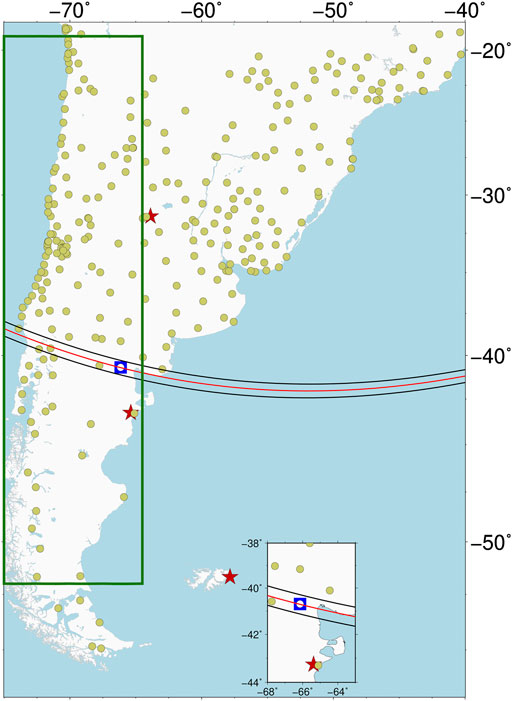
FIGURE 1. GNSS permanent stations (green circles) and geomagnetic observatories (red stars, namely PIL, TRW and PST from north to south), GNSS station and magnetometers installed in Valcheta, Río Negro (white circle and blue square). The red and black lines correspond to the center and the limits of eclipse totality path, respectively. Green box identifies the region used for latitude behavior analysis, which is shown in Section 3.1.
In addition to the magnetometers that were specifically placed for the observational campaign, we analyzed data from permanent geomagnetic observatories closest to the totality path. The nearest observatory is Trelew (TRW), which is located 290 km away from Valcheta, showing 93% solar occultation during the eclipse. Two other observatories were analyzed in which the occultation was 64.5%: Pilar (PIL) and Puerto Stanley (PST). Both are located symmetrically, approximately 1,000 km away from the totality path. However, the distance and magnitude of the eclipse at these two observatories contributed against their being suitable locations for testing the theoretical model used. We also checked data from Tristan da Cunha (TDC) with an occultation percentage of 89.84% but it was finally not considered for the analysis because the eclipse took place almost at dusk at this location and no GNSS data were available. All of these observatories participate in the International Network of Real-Time Magnetic Observatories (INTERMAGNET). The only exception is TRW, which is managed by our laboratory at FCAG and is momentarily not participating in this network due to an intermittent lack of data. All of the geomagnetic data was obtained from the INTERMAGNET data site. As was already described in (Meza et al., 2021), we selected the 1-min sample rate for the X, Y, Z components and total Field F.
In this section, we summarise the procedure that was used to compute VTEC values from GNSS observations; further details can be found in (Meza et al., 2021). We assume that all of the free electrons in the ionosphere are concentrated in a spherical shell of a finite thickness around Earth. The altitude of this spherical layer is usually set to the height of maximum electron density, which lies at approximately 450 km. The intersection point of the receiver-satellite line with the ionospheric layer is called the ionospheric pierce point. Using the GNSS multi-frequency observables it is possible to obtain the phase-code delay ionospheric observable, along with the geographic latitude and the sun-fixed longitude of the ionospheric pierce point, zenith angle, azimuth angle, and time for each satellite over each GNSS station. Finally, slant total electron content (STEC) is computed after the calibration of the ionospheric phase-code delay. For this last step, a constant value for each satellite-receiver arc is estimated and is then substracted from the phase-code delay (Ciraolo et al., 2007; Meza et al., 2009). STEC is mapped into VTEC by means of an obliquity factor (cos z′), where z′ is the zenithal angle of the slant path at the ionospheric piercing point.
Once the VTEC values were obtained, we followed the steps outlined in (Meza et al., 2021) to: 1) derive spatial averaging and time variations during the day of the eclipse VTECEcl and reference days VTECRef; and 2) perform the analysis on the net eclipse VTEC signal to derive the maximum effective VTEC depletion ΔVTECmax = max(VTECRef - VTECEcl) and Δt2 = t2 − t0—i.e., the delay between the maximum Solar obscuration at t0 and the instant when ΔVTECmax takes place (t2). We had to introduce a few changes due to the uneven spatial coverage and smaller number of GNSS stations. First, to improve statistics on geographical bins, we increased their size to 2 × 2° and we set the degrade time resolution to 3 min. Second, we resorted to quality control on the results of ΔVTECmax and Δt2 for geographical bins where data are too scarce and/or noisy as to provide reliable values. This was done by building two independent masks: the first identifies locations where the reduced χ2 goodness of fit indicator exceeded a threshold of 1.5, and the second is built by visual inspection to detect grid points where lack of data yield meaningless results.
The variability of the geomagnetic field component, which is produced by the eclipse effect, is only a few nanoteslas. Therefore, the geomagnetic conditions in which the eclipse develops have to be thoughtfully analyzed. The standard procedure states that the geomagnetic field variations induced by the solar eclipse are estimated from the X, Y, Z geomagnetic components. The geomagnetic field variability is defined as the difference between the values obtained during the eclipse event and the reference values, in which the reference field intensities are obtained using a mean value derived from the nearest quiet geomagnetic days. Additionally, to eliminate the intrinsic regular daily variabilities of the eclipse day with respect to the reference, the linear trend must be removed using a first-order polynomial fit (Malin et al., 2000; Meza et al., 2021). The need for this detrending is clearly shown in Figure 2A. Finally, the geomagnetic field variations produced by the solar eclipse, ΔX, ΔY, and ΔZ are computed.
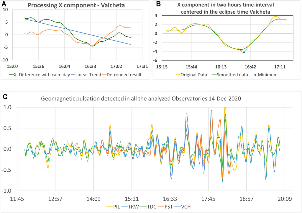
FIGURE 2. Geomagnetic analysis: (A) A graphical example of detrending the curve obtained after taking difference between the eclipse day and the quiet day to get a clean eclipse effect. (B) Example of the effect produced by the non-eclipse-related perturbation on the X component. (C) Geomagnetic pulsation detected in the five observatories analyzed, verifying that the perturbation noticed in (B) is not related to the eclipse effect. All vertical axis are in nT and the horizontal axis in UT.
In the case of the Valcheta site (VCH), the traveling restrictions imposed due to the Covid-19 pandemic made collecting data from several quiet days unfeasible. However, combining data from December 13th and 15th, both geomagnetically quiet (http://geomag.bgs.ac.uk) provided a good reference curve. Additionally, this reference was checked against the same obtained for TRW permanent geomagnetic station for consistency. A consistency check was also made by comparing the total field computed from the fluxgate measurements against the observations of the total field magnetometer.
Visual inspection of the eclipse day curves revealed the presence of a superimposed oscillation of variable amplitude. To rule out any dependence with the eclipse event itself, we inspected data from other geomagnetic observatories and found that the oscillation was also present and almost perfectly synchronized in time for the total field F measurements (Figure 2C). This appears to correspond to geomagnetic ULF pulsations of the type Pc5 (Jacobs et al., 1964). Because the eclipse perturbations are small enough to be affected by this signal, the eclipse day data was smoothed using a 29-point Gaussian filter (σ = 5.5 min) to ensure that the curve to be analyzed is free of noise. The impact of this ULF pulsation can be visualized as a strong negative peak in the X component that occurs at 16:36 UT, which is near the maximum eclipse occultation in the observatories of interest. If it was not filtered (due to the comparable magnitude of both phenomena), then it would affect the results; as shown in Figure 2B for the case of the X component in VCH.
On December 14th, an X class C4.0 flare occurred between 14:09 and 14:56 UT. However, the flare was too weak and took place before the eclipse event, so the increase in electron density due to the extra radiation does not impact geomagnetic variability.
The classical Ashour-Chapman model with modifications (Ashour and Chapman, 1965; Hvoz̆dara and Prigancová, 2002) is considered to analyze the geomagnetic components variability and its relationship with the relative VTEC decrement in the region of eclipse obscuration. A low-conductivity ionospheric spot is used as the Ashour-Chapman model of a thin current sheet model with the arbitrarily directed undisturbed electric field E0 (the direction of the equivalent Sq current system is assumed similar to E0). Three parameters are considered in the theoretical model of the geomagnetic disturbance (Hvoz̆dara and Prigancová, 2002): the angle between x-axis (towards geographic North) and E0 (ϵ), the distance from the observatories and the center of the eclipse-induced conductivity spot (δ), and the degree of the TEC decrease caused by the solar eclipse (κ). Table 1 shows the values of the three parameters that were used to calculate the geomagnetic disturbance for the different geomagnetic stations.
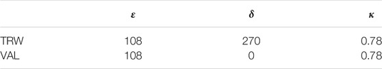
TABLE 1. The parameters used in the theoretical model of geomagnetic eclipse-disturbance: ϵ is the angle between x-axis (to geographic North) and E0; δ is the distance from the observatories and the center of the eclipse-induced conductivity spot (in km), and κ is the degree of the VTEC decrement caused by the solar eclipse.
The shadow path, as seen in Figure 1, extends over a relatively narrow patch of land in the southernmost part of South America, which prevents detailed analysis of variations along the eclipse track. Meanwhile, the availability of GNSS stations northwards provides an opportunity to study the changes in ΔVTEC due to variations in the occultation percentage, which diminishes perpendicularly to the shadow path (i.e. with latitude) and different latitudinal ionospheric behavior. Figure 3 shows the geographical distribution of the relative value of ΔVTECmax (in percentage units). Spatial coverage is not 100% complete due to a combination of fewer GNSS stations towards south and south-east, and low signal-to-noise ratio towards northeastern region. The largest values for relative ΔVTECmax are located westwards along the eclipse trace, and a second maximum can be found around 20°(approximately 10°geomagnetic latitude). The green rectangular box illustrates the size of the region where we have uniform coverage for our relative ΔVTECmax data, which will be used for our latitudinal analysis in what follows.
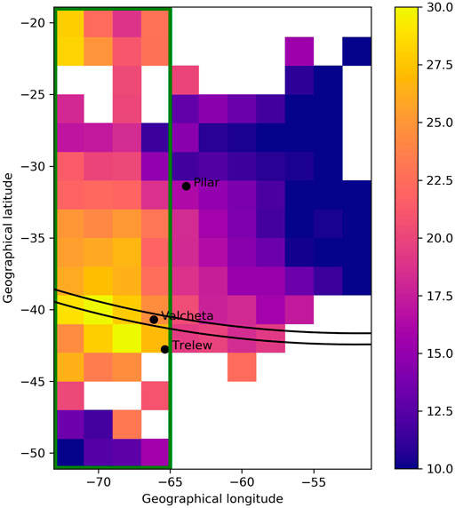
FIGURE 3. Plot of the geographical distribution of relative ΔVTECmax, displayed using color code from 10 to 30%. Empty bins are the result of quality check on individual fits due to poor GNSS stations coverage and/or low S/N ratio. The green rectangle identifies the region used for latitude behavior analysis shown in Figure 4.
Figure 4 shows the variation of the relative ΔVTECmax with latitude. The average values for each latitude bin, displayed as green boxes, show a descending trend when moving away from the shadow path, either southwards or northwards with maximum drops at −50° and −28°, respectively. A secondary increase in relative ΔVTECmax can also be observed towards −20°. The relative ΔVTECmax behavior with latitude may be explained by the eclipse attenuating effect on the ionization and by different ionospheric processes that tend to replenish the F2 layer from other altitudes. The steeper ΔVTECmax variation from the umbra towards high latitudes could be related to the high dip angle (I) favoring the downward diffusion flux (Le et al., 2009). As the intensity of diffusion scales with sin2I, an increased downward flux between plasmasphere and the F2 region would tend to compensate the lowered electron density at high latitudes. This downward flux occurs along the geomagnetic field lines from lower latitudes where plasmasphere has its highest density (Lee et al., 2013). The replenishment ions are driven along the geomagnetic lines from the relatively rich equatorial plasmasphere.
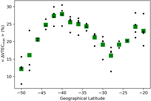
FIGURE 4. Plot of the observed average of relative ΔVTECmax with geographical latitude. Black dots show individual relative ΔVTECmax values for different longitudes within each latitude bin and green squares indicate average value within each bin.
According to (Le et al., 2009), the variation observed from low to equatorial latitudes could be related to the equatorial ionospheric response to the solar eclipse. The large depletion of electrons at low altitudes during the occultation is transmitted to higher altitudes thanks to the
Figure 5 shows our comparative analysis for VCH (top row) and TRW (bottom row). The left-hand panels display X, Y, and Z geomagnetic variation measurements for each observatory and the right-hand panels illustrate their corresponding model predictions (as detailed in the previous section). A comparison among sets for each location show an overall good qualitative agreement, and is able to explain the relative intensities and decreasing/increasing behavior for each component’s perturbations. In particular, the models are able to explain the relatively larger values for the X component variations for both locations, together with the faint variations for the Z component. The models can also explain different Y component behaviors in each location (almost negligible in Valcheta but evident in Trelew).
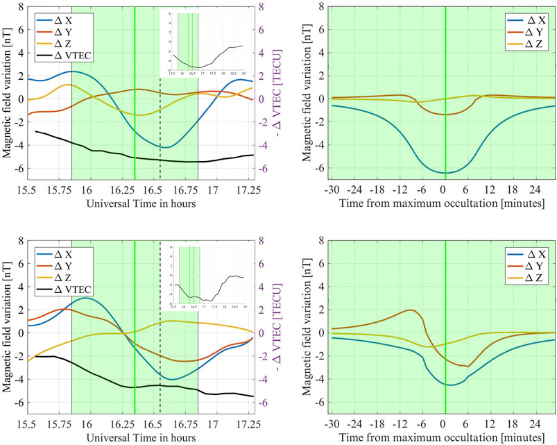
FIGURE 5. Geomagnetic variability detected from VCH (top) and TRW (bottom) observatories. The left-hand column shows the measurements of ΔX, ΔY, and ΔZ variations. Their intensities are labeled in the left-hand y-axis. The black curve shows ΔVTEC measurements with TECU intensities labelled in the right-hand axis. The top right-hand inset graphs in both panels show ΔVTEC behaviour over a longer time interval. The right-hand column shows the geomagnetic variability based on the Ashour-Chapman thin current sheet model.
There is, however, a notable difference in the response time between models and observations. While the models predict variations that are almost synchronized with eclipse occultation, with only a few minutes delay, the observatories detect these variations with a much larger time difference, approximately between 14 and 18 min. We can compare this temporal behavior with studies of the eclipse effect on ion density in the lower ionosphere. The dynamo current system, which is the principal contributor to the Solar quiet daily geomagnetic field variation (Sq), is directly related to the winds and the electrical conductivity in the E layer, the latter given by the electron density (N) in that region.
For the lower ionosphere, several authors record time delays between eclipse and electron density variations ranging from 2 to 5 min (Bullett and Mabie, 2018; Goncharenko et al., 2018), while others have found time delays of up 20 min above 90 km and E layer (Chandra et al., 1981; Belikovich et al., 2008; Bakhmetieva et al., 2017). Furthermore, an attempt to quantify this delay in terms of the so-called “sluggishness factor” was proposed by (Appleton, 1953), which explained the range of response delays in terms of different electron densities present in the ionospheric D and E layers.
A possible explanation for these delays could be related to the perturbation time constant of the ionosphere, τ, given by:
where N is the electron density, and α is the effective recombination coefficient. The value of the effective recombination coefficient is influenced by the ionic composition, the state of excitation, the temperature of the ionosphere, and the electron density. As indicated by several authors, α is usually 1–3 10–7 cm3/seg for the E layer (Wagner and Thome, 1972; Bates, 1988). Thus, according to the observed delays (almost 1,030 s), assuming that a noticeable effect (80% perturbation) becomes evident at 1.6 τ. Supposing α = 1.5 10–7 cm3/seg, it yields an N value of 1.1 104/cm3, which is not an unexpected value. Cooling, downwelling and atmospheric expansion processes originated by the movement of the moon shadow over the atmosphere can also contribute to this observed delay (Adekoya and Chukwuma, 2016). Unfortunately, the lack of instruments (e.g., ionosonde or incoherent radar) makes it impossible to directly obtain precise values for those parameters of the E layer at that moment, and therefore confirm or reject these results.
Figure 5 also includes the ΔVTEC variation curve on a 2 × 2° area over the corresponding geomagnetic observatories for comparison purposes. As reported in previous studies (Chandra et al., 1981), the response time of the VTEC changes is noticeably larger than that of the lower ionospheric layers that are linked with the geomagnetic variations. Considering that all of the ionospheric layers contribute to the TEC value, the ΔVTEC variation could be explained by the combination of chemical and dynamical (transport) processes. The VTEC decreases when the partial eclipse takes place. The reduction of VTEC during this period is mainly due to the decrease of photochemical production, which dominates in E and F1 layers. The decrease of VTEC continues even after the maximum occultation. This can be explained because the electron density decrease in the F2 layer and topside ionosphere are affected by dynamical processes, which could introduce a delay of upto 1 hour (Bienstock et al., 1970; Le et al., 2008).
We have devised and performed a dedicated campaign to obtain geomagnetic data from the actual shadow path of the Total Solar Eclipse that took place on December 14th, 2020 along the deserted Patagonia, in South America.
From the analysis of GNSS data, we found that the Solar Eclipse produced a variation in the relative value of ΔVTECmax up to 30%. The geographical distribution of the ΔVTECmax produced by the eclipse stresses that its amplitude is not only linked with the eclipse shadow path but is also linked with the actual ionospheric dynamics. This becomes evident in the presence of two local maxima of ΔVTECmax: the first matching the eclipse path and the second as we get close to the magnetic Equator, driven by the
Magnetic field variations were measured in two locations: the first placed right in the shadow path and the second less than 300 km away. We used a mathematical model based on the Ashour-Chapman theory to estimate the XYZ components variability of the geomagnetic field. These variations are comparable and compatible with actual observations, although we detect a noticeable delay with respect to the maximum occultation time. This retardment could be linked to the ionosphere’s sluggishness, which has been reported by several authors and found to reach up to 20 min long, mostly depending on electron density and changes in recombination coefficient.
To be able to fully study these delays, when planning future eclipse campaigns it is essential to include instrumentation that is able to characterize the electron density in the lower layers of the ionosphere.
Publicly available datasets were analyzed in this study. This data can be found here: www.intermagnet.org International Network of Real-Time Magnetic Observatories.
All authors listed have made a substantial, direct, and intellectual contribution to the work and approved it for publication.
The authors declare that the research was conducted in the absence of any commercial or financial relationships that could be construed as a potential conflict of interest.
All claims expressed in this article are solely those of the authors and do not necessarily represent those of their affiliated organizations, or those of the publisher, the editors and the reviewers. Any product that may be evaluated in this article, or claim that may be made by its manufacturer, is not guaranteed or endorsed by the publisher.
We acknowledge the hospitality and support from the city of Valcheta, particularly its Major Ms. Yamila Direne for opening access to the city during difficult times during the global Covid-19 pandemic. We also appreciate the extraordinary support from the FCAG under unpredictable circumstances reigning in December 2020. We thank Dr. Andreas Richter who facilitated the Trimble GPS receiver for this campaign. The GSM-19 magnetometer was loaned for this campaign by the Geomagnetism Department of the FCAG, Universidad Nacional de La Plata. Xavier M. Jubier eclipse maps were used for campaign planning and analysis (http://xjubier.free.fr). The results presented in this paper rely on data collected at magnetic observatories. We thank the national institutes that support them and INTERMAGNET for promoting high standards of magnetic observatory practice (www.intermagnet.org).
Adekoya, B. J., and Chukwuma, V. U. (2016). Ionospheric F2 Layer Responses to Total Solar Eclipses at Low and Mid-latitude. J. Atmos. Solar-Terr. Phys. 138-139, 136–160. doi:10.1016/j.jastp.2016.01.006
Afraimovich, E. L., Palamartchouk, K. S., Perevalova, N. P., Chernukhov, V. V., Lukhnev, A. V., and Zalutsky, V. T. (1998). Ionospheric Effects of the Solar Eclipse of March 9, 1997, as Deduced from Gps Data. Geophys. Res. Lett. 25, 465–468. doi:10.1029/98GL00186
Appleton, E. V. (1953). A Note on the "Sluggishness" of the Ionosphere. J. Atmos. Terr. Phys. 3, 282–284. doi:10.1016/0021-9169(53)90129-9
Ashour, A. A., and Chapman, S. (1965). The Magnetic Field of Electric Currents in an Unbounded Plane Sheet, Uniform except for a Circular Area of Different Uniform Conductivity. Geophys. J. Int. 10, 31–44. doi:10.1111/j.1365-246X.1965.tb03048.x
Bakhmetieva, N. V., Vyakhirev, V. D., Kalinina, E. E., and Komrakov, G. P. (2017). Earth's Lower Ionosphere during Partial Solar Eclipses According to Observations Near Nizhny Novgorod. Geomagn. Aeron. 57, 58–71. doi:10.1134/S0016793217010029
Bates, D. R. (1988). Recombination in the normal e and f layers of the ionosphere. Planet. Space Sci. 36, 55–63. doi:10.1016/0032-0633(88)90146-8
Belikovich, V. V., Vyakhirev, V. D., Kalinina, E. E., Tereshchenko, V. D., Chernyakov, S. M., and Tereshchenko, V. A. (2008). Ionospheric Response to the Partial Solar Eclipse of March 29, 2006, According to the Observations at Nizhni Novgorod and Murmansk. Geomagn. Aeron. 48, 98–103. doi:10.1007/s11478-008-1011-x10.1134/s0016793208010118
Bienstock, B. J., Marriott, R. T., John, D. E., Thorne, R. M., and Venkateswaran, S. V. (1970). Changes in the Electron Content of the Ionosphere. Nature 226, 1111–1112. doi:10.1038/2261111a0
Brenes, J., Leandro, G., and Fernández, W. (1993). Variation of the Geomagnetic Field in Costa Rica during the Total Solar Eclipse of July 11, 1991. Earth Moon Planet. 63, 105–117. doi:10.1007/BF00575100
Bullett, T., and Mabie, J. (2018). Vertical and Oblique Ionosphere Sounding during the 21 August 2017 Solar Eclipse. Geophys. Res. Lett. 45, 3690–3697. doi:10.1002/2018GL077413
Chandra, H., Sethia, G., Vyas, G., Deshpande, M., and Vats, H. (1981). Ionospheric Effects of the Total Solar Eclipse of 16 February 1980. Indian J. Radio Space Phys. - 1, 57–60.
Chen, G., Zhao, Z., Zhang, Y., Yang, G., Zhou, C., Huang, S., et al. (2011). Gravity Waves and Spread Es Observed during the Solar Eclipse of 22 July 2009. J. Geophys. Res. Space Phys. 116. doi:10.1029/2011JA016720
Cherniak, I., and Zakharenkova, I. (2018). Ionospheric Total Electron Content Response to the Great American Solar Eclipse of 21 August 2017. Geophys. Res. Lett. 45, 1199–1208. doi:10.1002/2017GL075989
Ciraolo, L., Azpilicueta, F., Brunini, C., Meza, A., and Radicella, S. M. (2007). Calibration Errors on Experimental Slant Total Electron Content (TEC) Determined with GPS. J. Geodesy 81, 111–120. doi:10.1007/s00190-006-0093-1
Cullington, A. L. (1962). Geomagnetic Effects of the Solar Eclipse, 12 October 1958, at Apia, western samoa. New Zealand J. Geology. Geophys. 5, 499–507. doi:10.1080/00288306.1962.10420103
Dang, T., Lei, J., Wang, W., Yan, M., Ren, D., and Huang, F. (2020). Prediction of the Thermospheric and Ionospheric Responses to the 21 June 2020 Annular Solar Eclipse. Earth Planet. Phys. 4, 231–237. doi:10.26464/epp2020032
Ding, F., Wan, W., Ning, B., Liu, L., Le, H., Xu, G., et al. (2010). Gps Tec Response to the 22 July 2009 Total Solar Eclipse in East Asia. J. Geophys. Res. Space Phys. 115, 1–8. doi:10.1029/2009JA015113
Goncharenko, L. P., Erickson, P. J., Zhang, S.-R., Galkin, I., Coster, A. J., and Jonah, O. F. (2018). Ionospheric Response to the Solar Eclipse of 21 August 2017 in Millstone hill (42n) Observations. Geophys. Res. Lett. 45, 4601–4609. doi:10.1029/2018GL077334
Hvoz̆dara, M., and Prigancová, A. (2002). Geomagnetic Effects Due to an Eclipse-Induced Low-Conductivity Ionospheric Spot. J. Geophys. Res. Space Phys. 107, 1–13. doi:10.1029/2002JA009260
Jacobs, J., Kato, Y., Matsushita, S., and Troitskaya, V. (1964). Classification of Geomagnetic Micropulsations. J. Geophys. Res. 69, 180–181. doi:10.1029/JZ069i001p00180
Jakowski, N., Stankov, S., Wilken, V., Borries, C., Altadill, D., Chum, J., et al. (2008). Ionospheric Behavior over Europe during the Solar Eclipse of 3 October 2005. J. Atmos. Solar-Terrestrial Phys. 70, 836–853. Measurements of Ionospheric Parameters influencing Radio Systems. doi:10.1016/j.jastp.2007.02.016
Kim, J.-H., and Chang, H.-Y. (2018). “Possible Influence of the Solar Eclipse on the Global Geomagnetic Field,” in Space Weather of the Heliosphere: Processes and Forecasts. Editors C. Foullon, and O. E. Malandraki, 335, 167–170. doi:10.1017/S1743921317007219
Knížová, P. K., and Mošna, Z. (2011). “Acoustic-gravity Waves in the Ionosphere during Solar Eclipse Events,” in Acoustic Waves. . Editor M. G. Beghi (Rijeka: IntechOpen), 303–320. chap. 14. doi:10.5772/19722
Kurkin, V. I., Nosov, V. E., Potekhin, A. P., Smirnov, V. F., and Zherebtsov, G. A. (2001). The March 9, 1997 Solar Eclipse Ionospheric Effects over the Russian Asian Region. Adv. Space Res. 27, 1437–1440. doi:10.1016/S0273-1177(01)00030-8
Le, H., Liu, L., Yue, X., and Wan, W. (2008). The Midlatitude F2 Layer during Solar Eclipses: Observations and Modeling. J. Geophys. Res. Space Phys. 113, 1–10. doi:10.1029/2007JA013012
Le, H., Liu, L., Yue, X., Wan, W., and Ning, B. (2009). Latitudinal Dependence of the Ionospheric Response to Solar Eclipses. J. Geophys. Res. Space Phys. 114, 1–11. doi:10.1029/2009JA014072
Lee, H.-B., Jee, G., Kim, Y. H., and Shim, J. S. (2013). Characteristics of Global Plasmaspheric Tec in Comparison with the Ionosphere Simultaneously Observed by Jason-1 Satellite. J. Geophys. Res. Space Phys. 118, 935–946. doi:10.1002/jgra.50130
MacPherson, B., González, S. A., Sulzer, M. P., Bailey, G. J., Djuth, F., and Rodriguez, P. (2000). Measurements of the Topside Ionosphere over Arecibo during the Total Solar Eclipse of February 26, 1998. J. Geophys. Res. Space Phys. 105, 23055–23067. doi:10.1029/2000JA000145
Malin, S. R. C., Özcan, O., Tank, S. B., Tunçer, M. K., and Yazici-Çakın, O. (2000). Geomagnetic Signature of the 1999 August 11 Total Eclipse. Geophys. J. Int. 140, F13–F16. doi:10.1046/j.1365-246X.2000.00061.x
Meza, A., van Zele, M. A., and Rovira, M. (2009). Solar Flare Effect on the Geomagnetic Field and Ionosphere. J. Atmos. Solar-Terr. Phys. 71, 1322–1332. doi:10.1016/j.jastp.2009.05.015
Meza, A., Bosch, G., Natali, P., and Eylenstein, B. (2021). Ionospheric and Geomagnetic Response to the Total Solar Eclipse on 21 August 2017. Adv. Space Res. (In press). doi:10.1016/j.asr.2021.07.029
Nevanlinna, H., and Hakkinen, L. (1991). Geomagnetic Effect of the Total Solar Eclipse on July 22, 1990. J. Geomagn. Geoelectr. 43, 319–321. doi:10.5636/jgg.43.319
Rishbeth, H. (1968). Solar Eclipses and Ionospheric Theory. Space Sci. Rev. 8, 543–554. doi:10.1007/BF00175006
Takeda, M., and Araki, T. (1984). Ionospheric Currents and fields during the Solar Eclipse. Planet. Space Sci. 32, 1013–1019. doi:10.1016/0032-0633(84)90057-6
Tyagi, T. R., Singh, L., Vijaya-Kumar, P. N., Somayajulu, Y. N., Lokanadham, B., and Yelliah, G. (1980). Satellite Radio beacon Study of the Ionospheric Variations at Hyderabad during the Total Solar Eclipse of 1980FEB16. Bull. Astronomical Soc. India 8, 69.
Keywords: solar eclipses, earth ionosphere, F-layer, E-layer, geomagnetic fields
Citation: Meza A, Eylenstein B, Natali MP, Bosch G, Moirano J and Chalar E (2021) Analysis of Ionospheric and Geomagnetic Response to the 2020 Patagonian Solar Eclipse. Front. Astron. Space Sci. 8:766327. doi: 10.3389/fspas.2021.766327
Received: 28 August 2021; Accepted: 15 November 2021;
Published: 03 December 2021.
Edited by:
Jorge Luis Chau, Leibniz-Institute of Atmospheric Physics (LG), GermanyReviewed by:
Massimo Materassi, National Research Council (CNR), ItalyCopyright © 2021 Meza, Eylenstein, Natali, Bosch, Moirano and Chalar. This is an open-access article distributed under the terms of the Creative Commons Attribution License (CC BY). The use, distribution or reproduction in other forums is permitted, provided the original author(s) and the copyright owner(s) are credited and that the original publication in this journal is cited, in accordance with accepted academic practice. No use, distribution or reproduction is permitted which does not comply with these terms.
*Correspondence: Amalia Meza, YW1lemFAZmNhZ2xwLnVubHAuZWR1LmFy
Disclaimer: All claims expressed in this article are solely those of the authors and do not necessarily represent those of their affiliated organizations, or those of the publisher, the editors and the reviewers. Any product that may be evaluated in this article or claim that may be made by its manufacturer is not guaranteed or endorsed by the publisher.
Research integrity at Frontiers
Learn more about the work of our research integrity team to safeguard the quality of each article we publish.