 Austin Brenner
 Tuija I. Pulkkinen
 Qusai Al Shidi
 Gabor Toth
- 1Department of Climate and Space Sciences and Engineering, University of Michigan, Ann Arbor, MI, United States
- 2Department of Aerospace Engineering, University of Michigan, Ann Arbor, MI, United States
- 3Department of Electronics and Nanoengineering, Aalto University, Espoo, Finland
Coupling between the solar wind and magnetosphere can be expressed in terms of energy transfer through the separating boundary known as the magnetopause. Geospace simulation is performed using the Space Weather Modeling Framework (SWMF) of a multi-ICME impact event on February 18–20, 2014 in order to study the energy transfer through the magnetopause during storm conditions. The magnetopause boundary is identified using a modified plasma β and fully closed field line criteria to a downstream distance of −20Re. Observations from Geotail, Themis, and Cluster are used as well as the Shue 1998 model to verify the simulation field data results and magnetopause boundary location. Once the boundary is identified, energy transfer is calculated in terms of total energy flux K, Poynting flux S, and hydrodynamic flux H. Surface motion effects are considered and the regional distribution of energy transfer on the magnetopause surface is explored in terms of dayside
1 Introduction
The past decades have greatly advanced our understanding of the dynamics in the space environment. The currently operative fleet termed by NASA as the Heliophysics System Observatory comprises several spacecraft in the solar wind (WIND, ACE, DSCOVR) and in the magnetosphere (Geotail, Cluster, THEMIS, MMS, AMPERE). Multipoint measurements can be made in electron (MMS), ion (Cluster), and mesoscales (THEMIS). Meanwhile, advances in global solar wind—magnetosphere—ionosphere simulations such as the SWMF (Space Weather Modeling Framework, Tóth et al., 2012), LFM (Lyon-Fedder-Mobarry model, Lyon et al., 2004), GAMERA (Grid Agnostic MHD for Extended Research Applications, Zhang et al., 2019), OpenGGCM (Open Geospace General Circulation Model, Raeder et al., 1996), and GUMICS (Grand Unified Magnetosphere Ionosphere Coupling Simulation model, Janhunen et al., 2012) have increased the level to which we can realistically reproduce dynamic processes in the different scales (Liemohn et al., 2018).
One of the key questions in heliospheric physics is to resolve how the solar wind energy enters the magnetosphere—ionoshere system to drive the dynamic space weather processes. In the solar wind, kinetic energy density (
While there is general agreement that magnetic reconnection at the magnetopause is the main conduit of energy entry into the magnetosphere—ionosphere system, the complexity of the processes and the multiple scales in which they occur still pose many challenges for producing reliable predictions of the space environment. Even without accounting for the complex inner magnetosphere processes that cannot be represented by pure MHD simulations, Pulkkinen et al. (2006) and Palmroth et al. (2006) explored magnetosphere reconnection under time varying solar wind drivers (solar wind speed and interplanetary magnetic field controlling the magnetospheric activity) and argued that magnetopause reconnection is a function of not only of the solar wind driver, but also depends on the prior level of geomagnetic activity. Furthermore, the magnetosheath electric field downstream of the bow shock is slightly larger in the quasi-parallel flank (Pulkkinen et al., 2016), suggesting that the foreshock waves may contribute to the way the plasma and magnetic field propagate across the bow shock (Pokhotelov et al., 2013). Furthermore, Nykyri et al. (2019) present an interesting case suggesting that a small-scale magnetosheath jet nudging the flank magnetopause can trigger a tail reconnection event leading to a substorm onset. Such sequences demonstrate the power of local disturbances to drive the magnetosphere through a large-scale reconfiguration process (Baker et al., 1999).
In this paper we return to the question of energy transfer into and out of a closed volume of the magnetosphere bounded by the magnetopause and a cross-section of the magnetotail at a given distance (20 RE). We use the University of Michigan Space Weather Modeling Framework (SWMF) simulation of a storm event on Feb 18–20, 2014, to examine how the energy transfer rates correlate with empirical proxies of energy entry, and how the energy input–output balance is maintained. Section 2 describes the simulation setup, Section 3 presents the observations of the event, Section 4 discusses the simulation analysis methodology, and Section 5 discusses the analysis results. Section 6 concludes with discussion.
2 The SWMF Geospace Simulation
We use the SWMF Geospace configuration (Tóth et al., 2012), which consists of the outer magnetosphere, inner magnetosphere and ionosphere electrodynamics components. The Geospace model can run faster than real time and is sufficiently accurate (Pulkkinen et al., 2013) to have been implemented by the NOAA Space Weather Prediction Center for operational use.
The solar wind and the magnetosphere are modeled by the BATS-R-US ideal MHD model (Tóth et al., 2012) with the adaptive grid resolution changing between 0.125 RE near the Earth and 8RE in the far tail. The simulation box in the Geocentric Solar Magnetospheric (GSM) coordinates extend from 32 RE to −224 RE in the X direction and ±128 RE in the Y and Z directions. The inner boundary is a spherical surface at radial distance R = 2.5 RE.
The inner magnetosphere’s non-Maxwellian plasmas are modeled by the Rice Convection Model (RCM) (Toffoletto et al., 2003), which solves the bounce- and pitch-angle-averaged phase space densities for protons, singly charged oxygen, and electrons in the inner magnetosphere. The MHD based model feeds the outer boundary condition and magnetic field configuration to the RCM, and the RCM plasma density and pressure values are used to modify the inner magnetosphere MHD solution (De Zeeuw et al., 2004). The 2-way coupling of BATS-R-US with RCM is performed every 10s. Including RCM provides a much improved representation of the ring current dynamics (Liemohn et al., 2018).
The ionospheric electrodynamics is described by the Ridley Ionosphere Model (RIM), which solves the Poisson equation for the electrostatic potential distribution at a two-dimensional ionospheric surface (Ridley et al., 2006). BATS-R-US feeds the RIM the field-aligned currents from the simulation inner boundary, and the ionospheric conductances are derived using the incoming field-aligned current intensity and location combined with background dayside and night-side conductances. The potential is set to zero at the lower latitude boundary at 10°. The RIM solves the Vasyliunas (1970) equation for the electric potential and feeds the electric field values back to the MHD simulation, giving a boundary condition for the velocity at the inner boundary. At the same time, the electric field values are fed to the RCM via a one-way coupling for determination of the drift speeds. The ionosphere and magnetosphere models are coupled every 5 s.
3 Event Overview
We focus on a time interval that comprises two interplanetary coronal mass ejections (ICME), which are a subset of a sequence of four that impacted the Earth during Feb 14–22, 2014. The geomagnetic activity that followed caused a complex sequence of depletions and enhancements of the van Allen belt electron populations (Kilpua et al., 2019). Here we focus on two consequtive ICMEs (second and third in the sequence) that were associated with a large geomagnetic storm and strong auroral region activity.
The period of Feb 18–20, 2014 contained two ICMEs that occurred back to back with the sheath region of the second ICME running into the ejecta of the first ICME. The first ICME impact was initiated by a shock at 0706 UT on Feb 18, and the ejecta arrived at 1545 UT. The second ICME shock arrived at 0356 UT, and the ejecta was observed between 1245 UT on Feb 19 and 0309 on Feb 20. Figure 1 shows the solar wind observations measured by the WIND spacecraft at the first Lagrangian point L1 point about 220 RE upstream of the Earth, and propagated to the bow shock as documented in the OMNI dataset (https://omniweb.gsfc.nasa.gov/). The yellow and green shading indicate the ICME sheath and ejecta respectively.
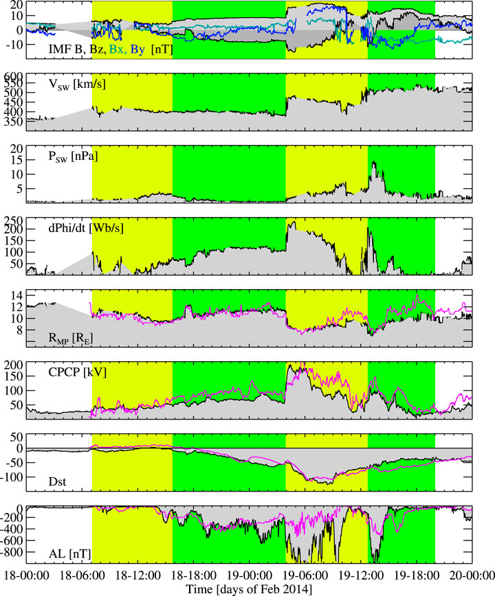
FIGURE 1. Observations of the solar wind driver and magnetospheric response (black line with shading) compared with SWMF Geospace results (magenta line). From top to bottom: IMF X (green), Y (blue) Z (black) components, total field magnitude (black); solar wind speed; solar wind pressure, Newell coupling function (see text); Magnetopause standoff distance (see text); cross-polar cap potential (see text); SMR (SuperMAG SYM-H index); SML (SuperMAG AL index). The yellow and green shading indicate the ICME sheath and ejecta respectively. The magenta lines in the bottom four panels show the SWMF Geospace simulation results.
The IMF magnitude hovered between 5 and 10 nT until the second shock, when the field magnitude increased to almost 20 nT. IMF BX was positive and small before the second ICME during which it turned strongly negative. IMF BY was close to zero before the second shock, which was associated with first strongly positive and then strongly negative BY. The BZ decreased during the first sheath to negative, but was mostly positive during the second ejecta.
The proton density was generally small at about 2 cm−3, but had a peak reaching above 10 cm−3 between about 1,200–1700 UT on Feb 18. The density increased gradually after the second shock, with peaks close to and above 30 cm−3 around 1000 and 1300 UT on Feb 19, respectively. The shock at 0356 UT on Feb 19 was also associated with a jump in the solar wind speed, from the nominal value at about 400 km/s during the first ICME, to slightly higher reaching above 500 km/s during the second ICME.
Figure 1 also shows the Newell et al. (2007) coupling parameter, representing the rate of change of magnetic flux at the nose of the magnetopause, and is an often used measure of the energy input from the solar wind into the magnetosphere—ionosphere system. The Newell function can be written in the form
where θ = tan−1(BY/BZ) is the IMF clock angle and
The following panels of Figure 1 show the magnetospheric response to the solar wind driving. A proxy for the subsolar magnetopause standoff distance RMP is given by the empirical Shue et al. (1998) model
where P is the solar wind dynamic pressure P = ρV2, ρ is the plasma mass density, and the factor 1.498 = 0.184 8.14 used in the original paper. While the first ICME did not cause major compression of the magnetopause, the sheath region of the second ICME pushed the magnetopause to near 8 RE, and the arrival of the ejecta compressed the magnetopause even closer to the Earth.
The sixth panel of Figure 1 shows an empirical proxy for the cross-polar cap potential (CPCP) given by Ridley and Kihn (2004) as a function of the polar cap index (PCI) measured in the northern polar cap (Thule station) and season. In this formulation, the CPCP is given in the form
where the time of year is scaled as T = 2π(NMONTH/12) and the numbering of months starts from zero (Jan = 0, Jul = 6). The polar cap potential was above 50 kV for the early part of the interval, but peaked at nearly 200 kV following the second shock, reducing to below 50 kV as the IMF turned northward.
The two bottom panels show the storm time index SYM-H and the auroral electrojet index AL, measuring the intensity of the ring current and westward ionospheric current, respectively. The sheath region of the first ICME had no marked effects on the inner magnetosphere or auroral currents, but both intensified strongly during the ejecta passage during the latter part of Feb 18. The second ICME sheath region in the interval was characterized by strongly southward IMF, and consequently drove very strong auroral currents and led to strong enhancement of the SYM-H index. The second ICME ejecta was associated with recovery of the ring current as well as quieting of the auroral currents.
The magenta lines in Figure 1 show the SWMF results in comparison with the observations. The SWMF Geospace simulation reproduces the subsolar magnetopause position to high accuracy with the exception of a diversion during the latter part of Feb 19th. The polar cap potential agrees quite well with the Ridley and Kihn (2004) empirical proxy. While the SYM-H index is quite well reproduced by the simulation, the simulation AL index does not reach the observed very high intensity during the second ICME sheath region.
4 Magnetospheric Boundary Motion
Several of the Heliophysics System Observatory spacecraft were monitoring the dynamics of the magnetospheric boundaries at the time of the storm. The Cluster 4-spacecraft constellation as well as Geotail were on the dayside, traversing through the bow shock and magnetopause. The three inner THEMIS spacecraft A, D, and E had their apogee on the dayside skimming the dayside magnetopause. THEMIS B and THEMIS C were in the dawn flank, moving outward toward the nominal bow shock location. Figure 2 shows the spacecraft trajectories in the GSM equatorial plane projection during the 2-day period. The grey shadings indicate a range of magnetopause and bow shock positions that empirical models predict for conditions that were observed during the interval.
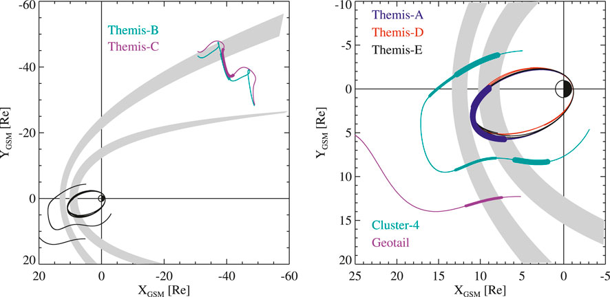
FIGURE 2. Spacecraft trajectories in the GSM X−Y plane during Feb 18–20, 2014. The grey shadings show a range of magnetopause and bow shock locations based on the range of solar wind conditions during the period. The thickest line segments show periods when the SCWeb locator places the trajectory within 2 RE from the magetopause, the medium thick segments show periods when the trajectory is within 2 RE from the bow shock position.
In order to examine how well the SWMF Geospace simulation reproduces the magnetospheric boundary locations during this interval, we use observations from all five THEMIS craft, from Geotail, and from Cluster 4. Figures 3–5 show magnetic field magnitude observations and simulation results. The vertical lines point out key times when there were changes in the solar wind and IMF (shown in black solid lines) or in the ground-based magnetic indices (substorm onsets, shown with dotted lines).
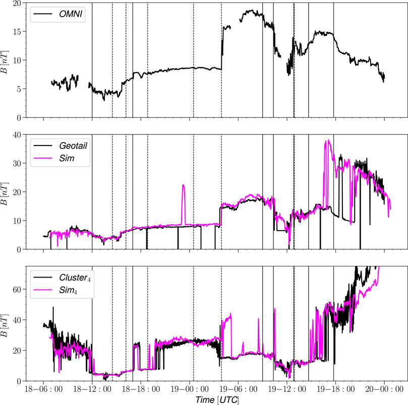
FIGURE 3. Magnetic field magnitude trace observation (black) vs simulation (magenta) Geotail and Cluster 4.
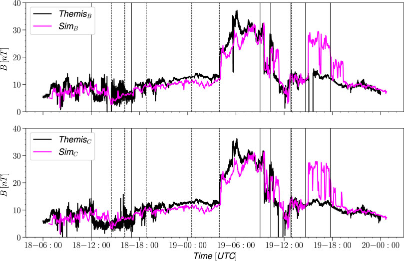
FIGURE 4. Magnetic field magnitude trace observation (black) vs simulation (magneta) Themis B and C.
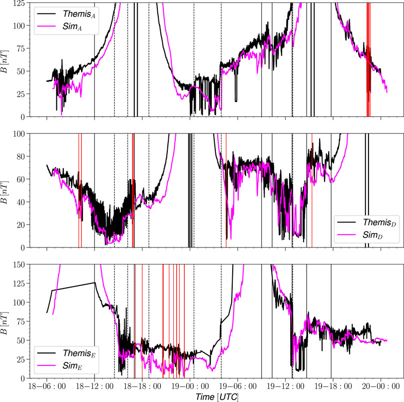
FIGURE 5. Magnetic field magnitude trace observation vs simulation Themis A, D, and E. Vertical red lines indicate crossings as determined by Staples et al. (2020).
Figure 3 shows the Geotail and Cluster-1 measurements of the magnetic field magnitude (the Cluster craft were close together, and show essentially similar behavior). The top panel repeats the OMNI IMF magnitude for reference. Geotail was in the solar wind, traveling inbound, monitoring the near-shock IMF until entering into the magnetosheath at about 20 UT on Feb 19. Cluster crossed from the magnetopause into the magnetosheath at around 07 UT and into the solar wind at around 12 UT on Feb 18. Cluster showed a brief encounter with the magnetosheath around 18 UT, a longer encounter between 20 UT on Feb 18 and 04 UT on Feb 19, and exited to the solar wind with the arrival of the sheath region of the second ICME which was associated with a strong compression of the magnetosphere. On its inbound path, Cluster crossed back to the magnetosheath at about 17 UT and into the magnetosphere at about 20 UT on Feb 19.
Figure 4 shows the THEMIS B and THEMIS C measurements at the dawn flank, close to the bow shock as demonstrated by the field values close to the IMF value combined with foreshock fluctuations. Both craft recorded a strong enhancement of the magnetic field in response to the increased IMF magnitude at about 04 UT on Feb 19 exceeding that of the IMF, indicating that the craft crossed the shock into the magnetosheath. As the IMF magnitude decreased, the THEMIS spacecraft returned to the solar wind.
Figure 5 shows the three inner THEMIS spacecraft observations of the dayside magnetospheric magnetic field. The large changes in IMF magnitude are seen as compression and relaxation in the dayside magnetic field as observed by all three spacecraft. Following the strongest compression period, THEMIS D and E crossed into the magnetosheath and during brief periods even to the pristine solar wind.
In each of the figures, the SWMF simulation results for the spacecraft locations are shown with magenta lines. In general, the boundary crossings associated with the inward motion of the magnetopause as the field magnitude increases are well reproduced by the simulation, while there are some timing differences associated with the boundary crossings.
The Geotail and Cluster virtual spacecraft time series match closely with observations other than brief enhancements, for the Geotail spacecraft around 23 UT on Feb 18 and for Cluster 4 most significantly shortly after 4 UT. Both simulation time series also show an early enhancement of B near the end of the simulation as they approach the magnetopause, indicating that the model magnetopause was slightly further out than the real one.
For THEMIS B and C, the only major difference between the simulation and observations is during the second ICME ejecta, when the simulation shows that the THEMIS location is immersed in the magnetosheath, shown as a strong and rapid increase and decrease of the simulated magnetic field magnitude between about 01 and 05 UT on Feb 19. The fluctuating field magnitude especially observed by THEMIS C is indicative of the spacecraft location very close to the bow shock, indicating that the simulation is likely showing only a minor deviation from the real location of the bow shock. The virtual spacecraft results of for the dayside THEMIS probes A, D, and E show minor timing errors and an overall lack of high-frequency oscillations in the magnetic field magnitude.
In Figure 5, times when the spacecraft locator (Staples et al., 2020) predicted magnetopause crossings are marked with red vertical lines (Figure 2). The local B magnitude average near the identified magnetopause crossings gives an indication that the magnetopause location is well reproduced with the simulation.
5 Boundary Identification in the Simulation
In order to quantify the energy transfer into the magnetosphere, we need to identify the magnetopause surface in the simulation. While the magnetopause can be topologically defined as the boundary between open and closed field lines in the dayside, it is often not a practical way to define the surface beyond the (quasi)dipolar region. In this work, the magnetopause identification was done via a field variable iso-surface of a modified plasma β parameter, which includes the MHD ram pressure (P = ρV2) as part of the plasma pressure,
where Pth is the plasma thermal pressure. This isosurface was expanded to include the fully closed field line region found by field line tracing techniques during simulation run time. The iso-surface generation technique was that provided by the “all triangles” creation method available in Tecplot software (Tecplot 360 EX 2020 R1, Version 2020.1.0.107285, Jul 13, 2020). The magnetospheric volume is closed by a cross-section of the tail at a constant X-value. Note that high β* plasma in the plasma sheet that is no longer on fully closed field lines can be found at distances within the constant X closure so the back surface was not always a perfect plane.
Figure 6 shows color contours of β* in the Y = 0 plane, which shows that there is a sharp gradient in the contour around the selected boundary value of 0.7. The sharp gradient demonstrates the insensitivity of the exact β* iso-surface level to the boundary location results. Indeed, multiple values of β* were tried and 0.7 was selected in order to push the boundary as far out as possible without pushing the dayside boundary sunward of the last closed fieldline, where β* can drop significantly. If this effect was compensated for separately, any value between 0.1 and 1.5 should yield similar results.
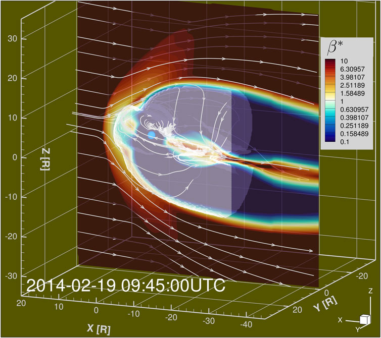
FIGURE 6. 3D snapshot of total energy transfer vector K flowfield with meridional cut showing color contours of β*. Translucent structure represents identified magnetopause surface out to −20Re in the x direction.
The complete closed 3D surface was split into dayside, flank, and tail subsections such that the dayside corresponds to the region with X > 0, the tail cross-section is defined by X = Xmin mostly in the YZGSM plane, and the flank is the remaining magnetopause surface area between the terminator and X = Xmin. The top panels of Figure 7 show the identified surface with dayside highlighted in light blue, magnetotail lobes in dark blue, and the tail cross section at Xmin = −20RE in purple. These surfaces combined form a closed surface that we use to examine energy flow into and out of the (inner part) of the magnetosphere.
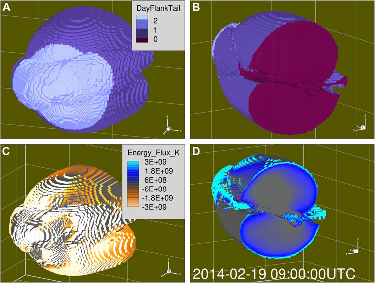
FIGURE 7. (A,B) show spatial breakdown of Dayside, Flank, and Tail subsections. (C,D) show energy flux into and out of the magnetosphere volume normal to the surface.
6 Energy Transfer Through a Simulation Surface
The total energy density U within a plasma volume is given in the MHD limit as
where γ = 5/3 is the ratio of specific heats. The corresponding total energy flux vector K is then given by
In order to examine the relative contributions of the plasma and electromagnetic processes, we re-arrange the equation to a sum of hydrodynamic energy flux H and Poynting flux S = (E × B)/μ0 to read
The energy transfer through the boundary specified in the previous section is given by the component of the energy fluxes normal to the boundary (K⋅ n), using the convention that the surface normal n points outward. The total energy flux rate is then obtained by integration over the entire surface area: Ktot = ∫AK⋅ dA. Using this notation, negative values of the flux through the surface (K⋅ n < 0) indicate total energy injection through the magnetopause into the magnetosphere. The time rate of change of the total energy enclosed within the boundary is then given as the net transport across the surface.
At times when the solar wind is rapidly changing and the magnetopause undergoes rapid compression or expansion, it is necessary to include the boundary motion into the equation. This can be done using the Reynolds transport theorem that describe the time rate of change of the total energy—the energy that is added to and lost from the volume enclosed by a surface in motion. Using the Reynolds transport theorem, the time rate of change of the total energy density (U) within the volume enclosed by the magnetopause (including the tail cross section closing the surface) can be written in the form
where q is the surface velocity. Note that only the normal component of the surface velocity q⋅ n matters. We also note that this equation does not account for the coupling to the inner magnetosphere module, which will also alter the energy density from the ideal MHD value. However, the right hand side captures all energy transfer effects at the magnetopause boundary, which is the focus of this study.
The surface is determined at discrete times, which means that the surface velocity has to be determined from a discrete approximation. We approximate the energy change associated with the moving boundary as a volumetric integral between the two surfaces:
where δt = tn+1−tn is the time difference between times tn and tn+1, and δV is the signed volume between the magnetospheric surfaces at the two times. Figure 8 illustrates the sign convention for this contribution to the energy transfer. This method allows us to compute energy addition and loss due to the boundary motion separately for the dayside, flank, and tail regions.
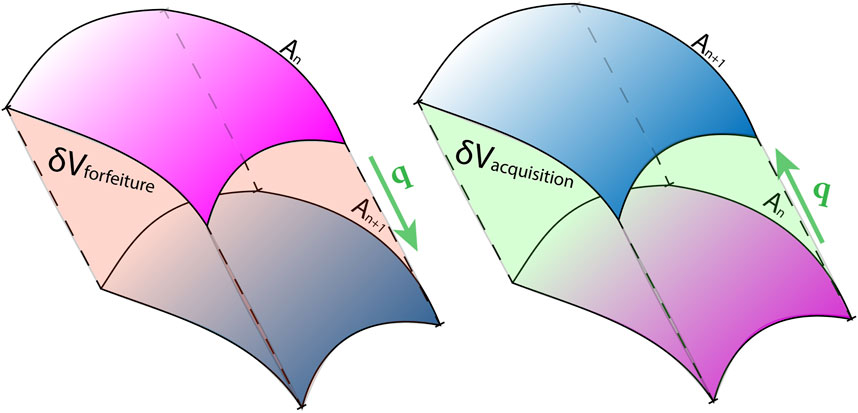
FIGURE 8. At each time step the energy density is integrated over δV representing the volume that will be acquired and/or lost in the next time step. Acquisitions and forfeitures are included in integrated flux of energy injected or escaped respectively. The local surface velocity is indicated by the vector q. The normal distance between the surfaces is (q ⋅ n)δt (Eq. 9).
The streamlines in Figure 6 show the total energy transfer vector K, and demonstrate that the energy transfer vectors penetrate well into the identified surface before turning, giving further evidence that the determination of energy at the boundary is insensitive to the exact value of β*. The bottom panels of Figure 7 show, at one given time instant, the energy flux into the magnetosphere (left) and out of the magnetosphere and through the magnetotail (right).
7 Stormtime Energy Transfer
Figure 9 shows integrated energy transfer through the entire magetopause surface broken down by type and sign. The top panel shows the total energy transfer rates, demonstrating that the net injection (brown) and escape (magenta) closely trace each other (with opposite signs). This indicates that there is much more energy flowing through the system than building up or escaping from inside the system. The net energy transfer (grey) shows short (of the order of a few hours) excursions of imbalance, but the average values are smaller than the totals by at least a factor of two.
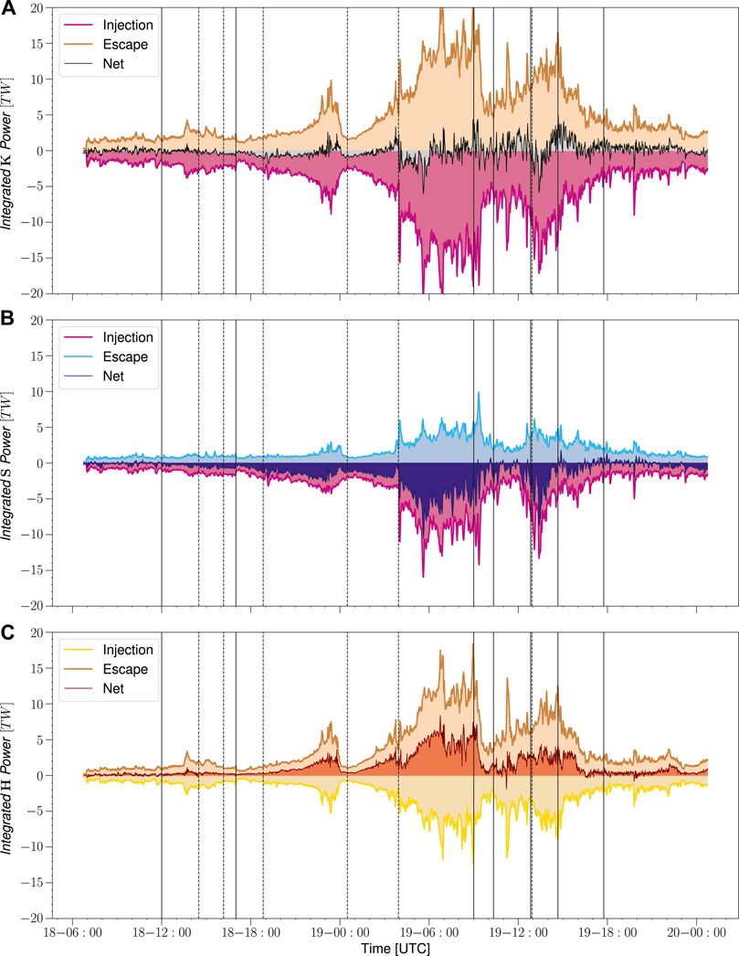
FIGURE 9. Full surface energy flux integration breakdown by type, (A): K (B): S (C): H (Eq. 7).
The next two panels of Figure 9 show the Poynting flux and hydrodynamic energy components of energy transfer. The energy injection is clearly dominated by the Poynting flux, while the Poynting flux has only a minor effect on the energy escape. On the other hand, hydrodynamic energy dominates the energy escape. Both types of energy as well as the total energy transfer rates clearly increase during the high ram pressure, high IMF magnitude portion of the event.
Figure 10 shows the contribution to the total energy transfer solely from the moving surface, using the right hand side of Eq. 9. The net energy transfer from the combined static and motional effects is shown in grey shading for comparison. The motional contributions of energy injection and escape are often unbalanced, which results the surface motion making a major contribution to the net totals. The top panel showing the solar wind ram pressure demonstrates a clear correlation with (changes in) the pressure and the boundary motion contribution to the energy transfer. As expected, during ram pressure spikes the surface volume decreases and energy escapes from the magnetosphere, especially during the oscillating behaviour of the volume beginning around 05 UT on the 19th (based on the relation between standoff distance and ram pressure the ram pressure and volume raised to −2.2 should scale about linearly; the Pearson correlation coefficient between the two is about 0.65). The first small enhancement in energy transfer due to the moving surface occurs during the first ICME ejecta and is due to enhanced energy in the flowfield, which cause relatively small fluctuations in surface velocity to transfer significant energy. The next enhancement results in net energy escape and is due to a dramatic shape change in the magnetosphere volume along the closed field line “wings” in the equatorial plane. Similar to the first energy enhancement the latter part of the event contains enhanced IMF magnitude which results in large changes in energy transfers due to the moving surface.
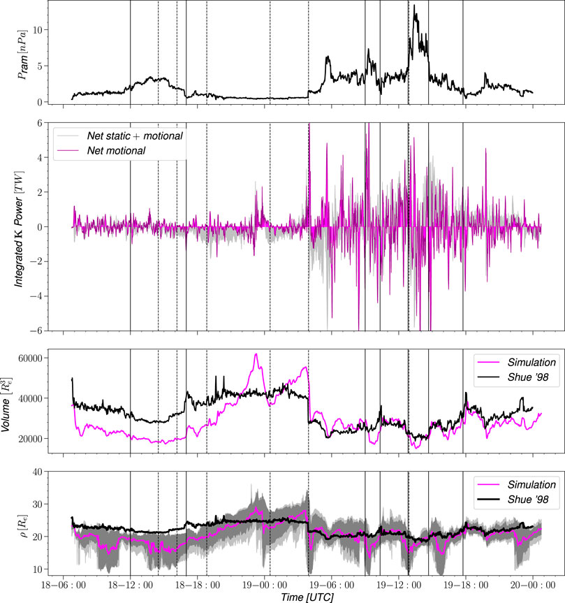
FIGURE 10. From top to bottom: Solar wind ram pressure; Integrated net power transfer due to surface motion effects only (magenta) compared with static and motion effects (grey); Magnetosphere volume integrated from simulation (magenta) compared with Shue 1998 model (black); Radial distance
The bottom panel of Figure 10 shows the volume enclosed by the surface created by the magnetopause and the tail cross section, using the Shue et al. (1998) model (black) and the surface identified from the SWMF Geospace simulation (magenta). While the two volumes generally correlate well, there are differences especially prior to when the strongest storm activity begins.
Figure 11 shows the contributions from the dayside, flank and tail stacked together to equal the total injection (negative) and escape (positive) for each type of energy. The top panel, which shows the total energy transfer indicates that the flank contribution can reach the level of the dayside energy transfer, while the tail cross-section consistently has only a small contribution. The second panel of Figure 11 shows that the dayside contribution to Poynting flux is quite steady throughout the event and is primarily energy escape, while the flank region contributes more to energy injection throughout the event and contains almost all of the high Poynting flux transfers both into and out of the magnetosphere. The bottom panel shows the breakdown for the total energy transfer by region in terms of percent contribution to better illustrate the tradeoff between the dayside and flank. The times when the flank contribution overtakes the dayside contribution appears to coincide with periods when high energy transfer on the surface is advected along the magnetopause surface from the dayside to the flank. These transient periods can also be seen in the third panel, in the distance between sharp drops in the dayside contribution in light blue and the total energy transfer indicated by the extremes of the curves.
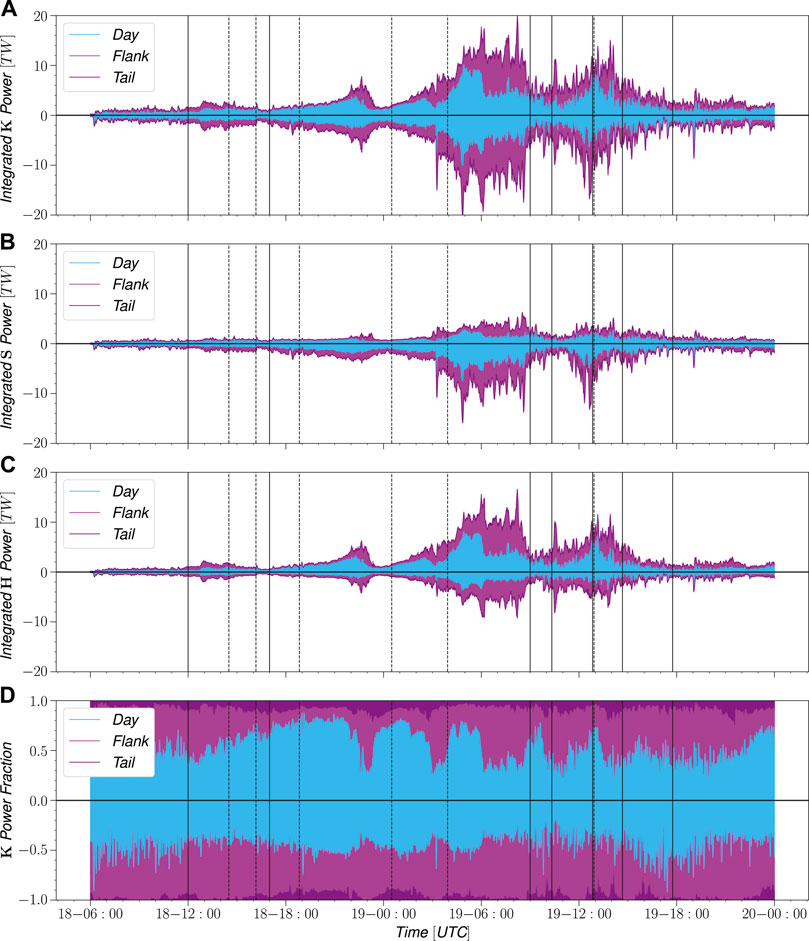
FIGURE 11. Energy injection and escape stacked by contribution. The first stack represents contribution from the dayside starting from 0. Next is the contribution from the flank starting from the dayside contribution and lastly is the contribution from the tail cap totalling to the injection and escape values found in Figure 9. As before the (A) represents total energy transfer, the (B) is Poynting flux and the (C) is the hydrodynamic energy flux. The (D) shows the relative contributions.
8 Discussion
In this paper, we have developed a method to identify the magnetopause boundary from a global MHD simulation, and calculate the energy transfer through that boundary into and out of the magnetosphere during a large geomagnetic storm. We examined the energy entry and exit separately, integrating the totals over the closed surface. Moreover, we examined contributions from the dayside (Sunward of the terminator), from the flanks (magnetopause between the terminator and X = −20 RE) and the tail cross section at the X = −20 RE plane, and computed the energy components related to the Poynting flux and hydrodynamic energy flux separately.
The most striking conclusion from our study is that most of the time, there is significant energy injection into the magnetosphere, but it is (almost) balanced by energy escaping the system. Our results show that most of the energy enters as Poynting flux, while the escape is dominated by the hydrodynamic energy flux (Figure 9). The energy transfer processes are most active in the dayside region (Sunward of the terminator), while the flank processes can be dominant at times. More events need to be analyzed to distinguish the conditions that dictate where the energy transfer processes take place. A lot of magnetospheric research has focused on processes in the magnetotail and estimating the energy that is associated with plasmoids leaving the system (e.g. Baker et al., 1996; Angelopoulos et al., 2013). However, our analysis shows that, in the large scale, the magnetotail plays only a minor role in the overall energy transfer. More detailed study focusing on substorm periods is needed to assess how important the tail contribution is during the substorm expansion phases.
Earlier work by Palmroth et al. (2003) shows an analogous analysis of magnetopause energy transfer in a global MHD simulation. Their results are based on a different method for magnetopause identification, they did not consider the effects of the boundary motion, and their simulation did not include the inner magnetosphere ring current contribution that in our case is represented via the coupling of the Rice Convection Model to the global MHD model. However, in the large scale, the results are analogous, showing the significant energy transfer along the tail flanks, and strongly and rapidly varying location and intensity of the energy transfer processes. While their tail integration extended out to 30 RE, and they did not include a magnetotail cross section, the overall magnitudes are comparable (Pulkkinen et al., 2008), which speaks to the robustness of the procedure. A more recent study by Jing et al. (2014) used SWMF with the magnetopause detection technique of Palmroth et al. (2006) and results support their findings, giving further confidence to the tools used for this study.
Observationally, the spaceborne measurements are not sufficient to yield global energy transfer rate estimates, but a significant body of work has assessed the role of the IMF components, the solar wind density and speed, and the solar wind electric field in the efficiency of the energy transfer process. Several coupling parameters relating the solar wind driver to the geomagnetic indices such as AL or Dst have been devised: The most widely used are the solar wind electric field EY = VXBZ (where VX is negative) (Burton et al., 1975), the rectified solar wind electric field ES = max (EY, 0) (so ES = 0 for BZ > 0) (McPherron et al., 2013), or the electric field parallel to the large-scale neutral line at the magnetopause (Pulkkinen et al., 2010). More complicated functions include the epsilon-parameter (ϵ = 107vB2 sin4 (θ/2)) introduced by (Akasofu, 1981) and the (Newell et al., 2007) coupling parameter given by Eq. 1.
The top panel of Figure 12 shows a comparison of the energy injection rate integrated over the entire surface compared with the Akasofu epsilon-parameter. While the magnitudes differ (the ϵ-parameter has empirical scaling that originally was matched with the Dst and AL contributions), the shape of the functions agree very well, indicating that the gating function sin4 (θ/2) in the ϵ-parameter is quite representative of the energy entry process.
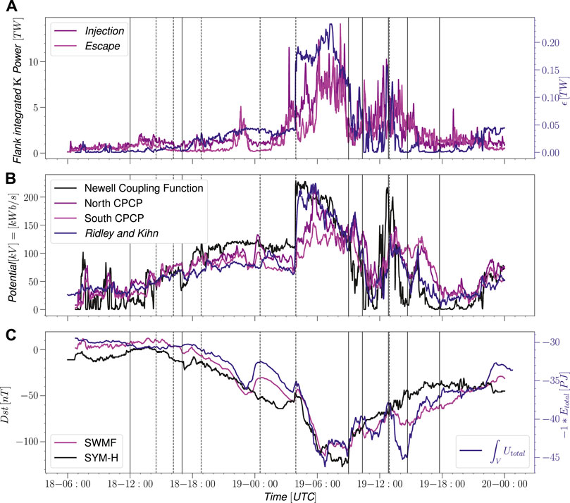
FIGURE 12. (A): Total energy transfer compared with Akasofu coupling parameter. (B): Cross polar cap potential from simulation and empirical model, compared with solar wind coupling of Newell. (C): Ground magnetic perturbation from simulation (magenta) and observation (black), plotted with energy density integrated over the defined magnetosphere volume.
The second panel of Figure 12 shows a similar comparison with the Newell coupling function and the polar cap potential in the simulation northern and southern ionosphere. Using the scaling for the Newell coupling parameter introduced by Cai and Clauer (2013), the magnitudes as well as the functional forms agree quite well, indicating that the Newell coupling function is a good proxy for energy that enters the polar ionospheres.
While the focus of this work is on the energy coupling at the magnetopause boundary, the energy density was also integrated over the entire volume to compare with the ground magnetic perturbation. The bottom panel of Figure 12 shows a high degree of correlation between the total energy and ground magnetic perturbation represented by the Dst index. This correlation is expected considering the theoretical formulation of the Dessler-Parker-Sckopke relation Dessler and Parker (1959) and the more general applications of the virial theorem as reviewed by Carovillano and Siscoe (1973). The clear connection between the total energy and ground magnetic perturbation underlines the importance of studying magnetosphere coupling in terms of energy transport.
The addition of the surface motion makes significant contributions to the energy transfer integrated totals despite having a relatively low amplitude due to the unbalanced contributions to energy injection and escape. Comparisons of the volume to the Shue model reveal a high degree of cylindrical asymmetry as the closed field line regions expand and are then lost, first by an internal process and again corresponding to a solar wind ram pressure spike. This effect can clearly be seen in the observations of ground magnetic perturbation and total energy around 04 UT on the 19th when the second ICME shock impacts. During this time a portion of the lateral closed field line region is lost, the volume undergoes rapid decrease, the simulated total energy sharply decreases in magnitude, and the energy spike is matched by both the simulated and ground based observation. Further studies are needed to understand what takes place in the magnetosphere during these fluctuations, to determine how much of the motion is due to magnetopause boundary oscillations. The results also show that the moving surface contribution is sensitive to the surrounding flowfield properties: When more energy density is contained in the magnetosheath, a relatively small fluctuation in surface position can result in large energy transfer.
9 Conclusion
In this work a 3D simulation was used to investigate the magnetosphere solar wind coupling during a very active event. In situ observations were combined with ground measurements of magnetic perturbations and empirical models were employed to better understand the expected behavior of the magnetosphere system and to validate the simulation results.
The main conclusions can be summarized as:
1) We have developed a robust method to assess the energy entry through the magnetopause into the magnetosphere. The energy entry is dominated by the Poynting flux, while the energy escapes from the system mainly in the form of hydrodynamic energy flux.
2) While dayside reconnection is an important process for the energy transfer, the energy transfer occurs throughout the magnetopause surface, with the flank contribution often being dominant.
3) Motion of the magnetopause causes an important contribution to the energy transfer rates, and thus cannot be ignored in the energy transfer rate computations.
4) The energy injection rate scales well with the Akasofu epsilon-function, while the total energy integrated within the closed volume defined by the magnetopause and a tail cross section (at X = −20RE) has a very similar functional shape to the Dst index, highlighting the ability of the Dst to capture the energy content within the magnetosphere.
5) The simulation magnetosphere shows significant asymmetry (deviation from rotational symmetry of the magnetopause surface). This leads to significant differences between volume estimates using the true magnetopause surface and empirical models especially during rapid variations in the driver parameters.
Data Availability Statement
The datasets presented in this study can be found at the University of Michigan Deep Blue repository. https://doi.org/10.7302/nxyj-7062.
Author Contributions
AB and QA, were responsible for running the simulation. AB, TP, QA, and GT contributed to analysis methodology conception. AB wrote and developed the analysis code. TP was responsible for event selection and initial event analysis. AB and TP were responsible for writing the manuscript. AB, TP, QA, and GT contributed to manuscript revisions leading to submitted version.
Funding
This research was funded through NSF grant number 2033563 and as part of the NASA DRIVE Center SOLSTICE (Grant Number 80NSSC20K0600).
Conflict of Interest
The authors declare that the research was conducted in the absence of any commercial or financial relationships that could be construed as a potential conflict of interest.
Publisher’s Note
All claims expressed in this article are solely those of the authors and do not necessarily represent those of their affiliated organizations, or those of the publisher, the editors and the reviewers. Any product that may be evaluated in this article, or claim that may be made by its manufacturer, is not guaranteed or endorsed by the publisher.
Acknowledgments
This work was carried out using the SWMF and BATS-R-US tools developed at the University of Michigan’s Center for Space Environment Modeling (CSEM). The modeling tools described in this publication are available online through the University of Michigan for download and are available for use at the Community Coordinated Modeling Center (CCMC) as well as through Github at https://github.com/MSTEM-QUDA.
References
Akasofu, S. (1981). Energy Coupling between the Solar Wind and the Magnetosphere. Space Sci. Rev. 28, 121–190. doi:10.1007/bf00218810
Angelopoulos, V., Runov, A., Zhou, X. Z., Turner, D. L., Kiehas, S. A., Li, S. S., et al. (2013). Electromagnetic Energy Conversion at Reconnection Fronts. Science 341, 1478–1482. doi:10.1126/science.1236992
Baker, D. N., Pulkkinen, T. I., Angelopoulos, V., Baumjohann, W., and McPherron, R. L. (1996). Neutral Line Model of Substorms: Past Results and Present View. J. Geophys. Res. 101, 12975–13010. doi:10.1029/95ja03753
Baker, D. N., Pulkkinen, T. I., Büchner, J., and Klimas, A. J. (1999). Substorms: A Global Instability of the Magnetosphere-Ionosphere System. J. Geophys. Res. 104, 14601–14611. doi:10.1029/1999JA900162
Burton, R. K., McPherron, R. L., and Russell, C. T. (1975). An Empirical Relationship between Interplanetary Conditions andDst. J. Geophys. Res. 80, 4204–4214. doi:10.1029/ja080i031p04204
Cai, X., and Clauer, C. R. (2013). Magnetospheric Sawtooth Events during the Solar Cycle 23. J. Geophys. Res. Space Phys. 118, 6378–6388. doi:10.1002/2013JA018819
Carovillano, R. L., and Siscoe, G. L. (1973). Energy and Momentum Theorems in Magnetospheric Processes. Rev. Geophys. 11, 289–353. doi:10.1029/RG011i002p00289
Chen, Y., Tóth, G., Cassak, P., Jia, X., Gombosi, T. I., Slavin, J. A., et al. (2017). Global Three‐Dimensional Simulation of Earth's Dayside Reconnection Using a Two‐Way Coupled Magnetohydrodynamics with Embedded Particle‐in‐Cell Model: Initial Results. J. Geophys. Res. Space Phys. 122, 10,318–10,335. doi:10.1002/2017JA024186
De Zeeuw, D. L., Sazykin, S., Wolf, R., Gombosi, T., Ridley, A., and Tóth, G. (2004). Coupling of a Global MHD Code and an Inner Magnetospheric Model: Initial Results. J. Geophys. Res. 109, 219. doi:10.1029/2003JA010366
Dessler, A. J., and Parker, E. N. (1959). Hydromagnetic Theory of Geomagnetic Storms. J. Geophys. Res. 64, 2239–2252. doi:10.1029/JZ064i012p02239
Janhunen, P., Palmroth, M., Laitinen, T., Honkonen, I., Juusola, L., Facskó, G., et al. (2012). The GUMICS-4 Global MHD Magnetosphere-Ionosphere Coupling Simulation. J. Atmos. Solar-Terrestrial Phys. 80, 48–59. doi:10.1016/j.jastp.2012.03.006
Jing, H., Lu, J. Y., Kabin, K., Zhao, J. S., Liu, Z.-Q., Yang, Y. F., et al. (2014). Mhd Simulation of Energy Transfer across Magnetopause during Sudden Changes of the Imf Orientation. Planet. Space Sci. 97, 50–59. doi:10.1016/j.pss.2014.04.001
Kilpua, E. K. J., Turner, D. L., Jaynes, A. N., Hietala, H., Koskinen, H. E. J., Osmane, A., et al. (2019). Outer Van allen Radiation belt Response to Interacting Interplanetary Coronal Mass Ejections. J. Geophys. Res. Space Phys. 124, 1927–1947. doi:10.1029/2018JA026238
Laitinen, T. V., Janhunen, P., Pulkkinen, T. I., Palmroth, M., and Koskinen, H. E. J. (2006). On the Characterization of Magnetic Reconnection in Global Mhd Simulations. Ann. Geophys. 24, 3059–3069. doi:10.5194/angeo-24-3059-2006
Liemohn, M., Ganushkina, N. Y., De Zeeuw, D. L., Rastaetter, L., Kuznetsova, M., Welling, D. T., et al. (2018). Real‐Time SWMF at CCMC: Assessing the Dst Output from Continuous Operational Simulations. Space Weather. 16, 1583–1603. doi:10.1029/2018SW001953
Lyon, J. G., Fedder, J. A., and Mobarry, C. M. (2004). The Lyon-Fedder-Mobarry (LFM) Global MHD Magnetospheric Simulation Code. J. Atmos. Solar-Terrestrial Phys. 66, 1333–1350. doi:10.1016/j.jastp.2004.03.020
McPherron, R. L., Baker, D. N., Pulkkinen, T. I., Hsu, T.-S., Kissinger, J., and Chu, X. (2013). Changes in Solar Wind-Magnetosphere Coupling with Solar Cycle, Season, and Time Relative to Stream Interfaces. J. Atmos. Solar-Terrestrial Phys. 99, 1–13. Dynamics of the Complex Geospace System. doi:10.1016/j.jastp.2012.09.003
Newell, P. T., Sotirelis, T., Liou, K., Meng, C.-I., and Rich, F. J. (2007). A Nearly Universal Solar Wind-Magnetosphere Coupling Function Inferred from 10 Magnetospheric State Variables. J. Geophys. Res. 112, a–n. doi:10.1029/2006JA012015
Nykyri, K., Bengtson, M., Angelopoulos, V., Nishimura, Y., and Wing, S. (2019). Can Enhanced Flux Loading by High‐Speed Jets Lead to a Substorm? Multipoint Detection of the Christmas Day Substorm Onset at 08:17 UT, 2015. J. Geophys. Res. Space Phys. 124, 4314–4340. doi:10.1029/2018JA026357
Nykyri, K., and Otto, A. (2001). Plasma Transport at the Magnetospheric Boundary Due to Reconnection in Kelvin-Helmholtz Vortices. Geophys. Res. Lett. 28, 3565–3568. doi:10.1029/2001GL013239
Palmroth, M., Janhunen, P., and Pulkkinen, T. I. (2006). Hysteresis in Solar Wind Power Input to the Magnetosphere. Geophys. Res. Lett. 33, L03107. doi:10.1029/2005GL025188
Palmroth, M., Pulkkinen, T., Janhunen, P., and Wu, C.-C. (2003). Stormtime Energy Transfer in Global MHD Simulation. J. Geophys. Res. 108, 1048. doi:10.1029/2002JA009446
Pokhotelov, D., von Alfthan, S., Kempf, Y., Vainio, R., Koskinen, H. E. J., and Palmroth, M. (2013). Ion Distributions Upstream and Downstream of the Earth's bow Shock: First Results from Vlasiator. Ann. Geophys. 31, 2207–2212. doi:10.5194/angeo-31-2207-2013
Pulkkinen, A., Rastätter, L., Kuznetsova, M., Singer, H., Balch, C., Weimer, D., et al. (2013). Community-wide Validation of Geospace Model Ground Magnetic Field Perturbation Predictions to Support Model Transition to Operations. Space Weather 11, 369–385. doi:10.1002/swe.20056
Pulkkinen, T. I., Dimmock, A. P., Lakka, A., Osmane, A., Kilpua, E., Myllys, M., et al. (2016). Magnetosheath Control of Solar Wind‐magnetosphere Coupling Efficiency. J. Geophys. Res. Space Phys. 121, 8728–8739. doi:10.1002/2016JA023011
Pulkkinen, T. I., Palmroth, M., Koskinen, H. E. J., Laitinen, T. V., Goodrich, C. C., Merkin, V. G., et al. (2010). Magnetospheric Modes and Solar Wind Energy Coupling Efficiency. J. Geophys. Res. 115, A03207. doi:10.1029/2009ja014737
Pulkkinen, T. I., Palmroth, M., and Laitinen, T. (2008). Energy as a Tracer of Magnetospheric Processes: GUMICS-4 Global MHD Results and Observations Compared. J. Atmos. Solar-Terrestrial Phys. 70, 687–707. doi:10.1016/j.jastp.2007.10.011
Pulkkinen, T. I., Palmroth, M., Tanskanen, E. I., Janhunen, P., Koskinen, H. E. J., and Laitinen, T. V. (2006). New Interpretation of Magnetospheric Energy Circulation. Geophys. Res. Lett. 33, L0701. doi:10.1029/2005GL025457
Raeder, J., Berchem, J., and Ashour-Abdalla, M. (1996). “The Importance of Small Scale Processes in Global MHD Simulations: Some Numerical Experiments,” in The Physics of Space Plasmas. Editors T. Chang, and J. R. Jasperse (Cambridge, Mass.: MIT Cent. for Theoret. Geo/Cosmo Plasma Phys.), 14, 403.
Ridley, A. J., Deng, Y., and Tóth, G. (2006). The Global Ionosphere-Thermosphere Model. J. Atmos. Solar-Terrestrial Phys. 68, 839–864. doi:10.1016/j.jastp.2006.01.008
Ridley, A. J., and Kihn, E. A. (2004). Polar Cap index Comparisons with AMIE Cross Polar Cap Potential, Electric Field, and Polar Cap Area. Geophys. Res. Lett. 31, a–n. doi:10.1029/2003GL019113
Shue, J.-H., Song, P., Russell, C. T., Steinberg, J. T., Chao, J. K., et al. (1998). Magnetopause Location under Exteme Solar Wind Conditions 103, 17,691–17,700doi:10.1029/98ja01103
Staples, F. A., Rae, I. J., Forsyth, C., Smith, A. R. A., Murphy, K. R., Raymer, K. M., et al. (2020). Do statistical Models Capture the Dynamics of the Magnetopause during Sudden Magnetospheric Compressions? J. Geophys. Res. Space Phys. 125, e2019JA027289. doi:10.1029/2019JA027289
Toffoletto, F., Sazykin, S., Spiro, R., and Wolf, R. (2003). Inner Magnetospheric Modeling with the Rice Convection Model. Space Sci. Rev. 107, 175–196. doi:10.1023/A:1025532008047
Tóth, G., van der Holst, B., Sokolov, I. V., De Zeeuw, D. L., Gombosi, T. I., Fang, F., et al. (2012). Adaptive Numerical Algorithms in Space Weather Modeling. J. Comput. Phys. 231, 870–903. doi:10.1016/j.jcp.2011.02.006
Vasyliunas, V. M. (1970). “Mathematical Models of Magnetospheric Convection and its Coupling to the Ionosphere,” in Particles and fields in the Magnetosphere. Editor B. M. McCormack (Dordrecht, Holland: D. Reidel Publishing), 60–71. doi:10.1007/978-94-010-3284-1_6
Keywords: space plasma, magnetopause, energy transfer, magnetosphere, substorm, poynting flux, MHD simulations
Citation: Brenner A, Pulkkinen TI, Al Shidi Q and Toth G (2021) Stormtime Energetics: Energy Transport Across the Magnetopause in a Global MHD Simulation. Front. Astron. Space Sci. 8:756732. doi: 10.3389/fspas.2021.756732
Received: 11 August 2021; Accepted: 27 September 2021;
Published: 15 October 2021.
Edited by:
Katariina Nykyri, Embry–Riddle Aeronautical University, United StatesReviewed by:
Bogdan Hnat, University of Warwick, United KingdomLaxman Adhikari, University of Alabama in Huntsville, United States
Copyright © 2021 Brenner, Pulkkinen, Al Shidi and Toth. This is an open-access article distributed under the terms of the Creative Commons Attribution License (CC BY). The use, distribution or reproduction in other forums is permitted, provided the original author(s) and the copyright owner(s) are credited and that the original publication in this journal is cited, in accordance with accepted academic practice. No use, distribution or reproduction is permitted which does not comply with these terms.
*Correspondence: Austin Brenner, YXVickB1bWljaC5lZHU=