
94% of researchers rate our articles as excellent or good
Learn more about the work of our research integrity team to safeguard the quality of each article we publish.
Find out more
REVIEW article
Front. Astron. Space Sci., 24 August 2021
Sec. Space Physics
Volume 8 - 2021 | https://doi.org/10.3389/fspas.2021.708940
This article is part of the Research TopicCold-Ion Populations and Cold-Electron Populations in the Earth’s Magnetosphere and Their Impact on the SystemView all 18 articles
 Kazue Takahashi1*
 Richard E. Denton 2
The technique to estimate the mass density in the magnetosphere using the physical properties of observed magnetohydrodynamic waves is known as magnetoseismology. This technique is important in magnetospheric research given the difficulty of determining the density using particle experiments. This paper presents a review of magnetoseismic studies based on satellite observations of standing Alfvén waves. The data sources for the studies include AMPTE/CCE, CRRES, GOES, Geotail, THEMIS, Van Allen Probes, and Arase. We describe data analysis and density modeling techniques, major results, and remaining issues in magnetoseismic research.
Mass density (denoted ρ) is a fundamental quantity of the magnetospheric plasma. The density controls the properties of various ion-scale plasma waves and the time scale of global magnetospheric processes. The density is also a key quantity in studying the ionospheric response to the solar activity and the coupling between the magnetosphere and the ionosphere. Despite the importance of ρ, its determination from particle data is difficult because no particle detector is capable of covering the full range of energies, pitch angles, and ion composition, which is necessary to obtain the density through moment calculation. This makes indirect techniques very valuable.
The idea of using ultralow-frequency (ULF) waves as a tool to estimate ρ, now known as magnetoseismology, was presented as early as the late 1950s (Obayashi and Jacobs, 1958) based on the magnetohydrodynamic (MHD) theory of magnetospheric ULF waves (Dungey, 1954). Both the shear mode (Alfvén waves) and compressional mode (fast magnetosonic waves) have been used in magnetoseismology. This paper describes Alfvén wave techniques, termed normal mode magnetoseismology (Chi and Russell, 2005). The publication of the cross-phase technique to determine the frequency of standing Alfvén waves (field line resonances, FLRs) (Waters et al., 1991) led to numerous magnetoseismic studies using ground magnetometer data. We will focus on data analysis and modeling techniques for spacecraft data. Readers are referred to Menk and Waters (2013) and Del Corpo et al. (2020) for results based on ground observations and to Denton (2006) for early results based on spacecraft observations.
The remainder of this paper is as follows. Section 2 presents the theoretical background and modeling approach. Section 3 presents data analysis results. Section 4 presents discussion, and section 5 presents the conclusions.
Techniques to infer mass density structures are well established in terrestrial and solar seismology. Our idea is to use similar techniques to infer the mass distribution in the terrestrial magnetosphere. The basic principle of magnetoseismology is that ρ is related to the frequency and mode structure of standing Alfvén waves. Figure 1 illustrates this relationship using a string model of magnetic field lines. The frequency of vibrations of the string (blue curves) is determined by the tension (restoring force) of the string and the mass (filled red circles) attached to the string. The discrete mass distribution is only for illustrative purposes. In reality, the mass is distributed continuously.
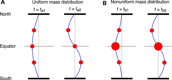
FIGURE 1. String analogy of standing Alfvén waves. The blue curves represent the field line, and the size of the filled red circles represents the mass density value. The string is tied at the northern and southern ends corresponding to the ionospheric footpoints of the field line. (A) Structure of the fundamental (left) and second harmonic (right) modes for the case of a uniform mass density distribution along the field line. The node or antinode is located at the equator (horizontal dashed line). The mode frequencies are denoted fa1 and fa2. (B) Same as (A) but for a mass density distribution that is peaked at the equator. The mode frequencies are denoted fb1 and fb2.
Figure 1A illustrates the fundamental and second harmonic modes for the case of a uniform mass distribution along the field line. The mode structure is a sine function for either harmonic, and the frequencies are related as fa2 = 2fa1. The time-of-flight calculation described below gives exact solutions of the mode frequency and structure for all harmonics.
Figure 1B illustrates the case of a nonuniform mass density distribution with a peak at the equator. In this case, the mode structure of the fundamental mode is not a sine function, and the frequency of the fundamental mode (fb1) is lower than fa1. However, the equatorial mass density does not affect the mode structure or the frequency of the second harmonic because the string displacement is zero (node) at the equator. As a consequence, the mode of the second harmonic is a sine function, the same as in Figure 1A. The mass density effects on the wave properties occur for higher harmonics also. This means that we can infer the mass density distribution from the frequencies and mode structures determined using spacecraft data.
To advance the concept illustrated in Figure 1 to magnetoseismology of the real magnetosphere, we obtain the relationship between the waves and ρ using the cold plasma MHD wave equation (e.g., Radoski and Carovillano, 1966)
where δE is the wave electric field and VA is the Alfvén velocity, which depends on the magnetic field B and ρ as VA =
Poloidal waves are detected also, but these waves have not been used much in magnetoseismology. Considering the fact that poloidal waves are not detected by ground magnetometers because of the ionospheric screening of high-m waves (Hughes and Southwood, 1976) and also the fact that the waves exhibit a different local time occurrence distribution than toroidal waves (Arthur and McPherron, 1981), poloidal waves could be a valuable resource in future magnetoseismic studies. Poloidal waves have the advantage of being excited nearly exclusively at the second harmonic (Cummings et al., 1969; Takahashi and McPherron, 1984; Anderson et al., 1990; Liu et al., 2013), reducing the uncertainty in harmonic mode identification. But a disadvantage to using poloidal waves is that the wave frequency depends on the radial pressure gradient, which is not always well determined (Denton, 2003, and references therein).
The magnetospheric magnetic field significantly differs from the dipole field at large distances or during geomagnetically disturbed periods, making it difficult to exactly solve Eq. 1. Fortunately, MHD-scale disturbances quickly settle to toroidal eigenmode oscillations (Allan et al., 1986; Lee and Lysak, 1989) through the FLR process (e.g., Chen and Hasegawa, 1974), and we can treat each field line to be an independent oscillator in the context of magnetoseismology. For example, we can use the time-of-flight approximation for the fundamental frequency f1 on a field line (Warner and Orr, 1979; Wild et al., 2005)
where s is distance along the field line and the integral is taken between the southern (S) and northern (N) ionospheric footpoints. In this approximation, there is no distinction between toroidal and poloidal frequencies, the frequency of the nth harmonic (fn) is equal to nf1, and the fn value is higher than that obtained by more accurate methods (Takahashi and McPherron, 1984). More accurate eigenmode solutions are obtained by numerically solving the equation
where ξi is the field line displacement associated with the wave and hi is the scale factor vector of the background magnetic field B, with the suffix i indicating the direction within the plane perpendicular to B (Singer et al., 1981). To solve this equation for a general magnetic field geometry, one selects two adjacent model magnetic field lines to specify the direction (polarization axis) of magnetic field perturbation. This flexibility is valuable in consideration of theoretical studies (Lee et al., 2000; Wright and Elsden, 2016) indicating that the polarization axis of toroidal waves is not tangential to the magnetic field L shells when the ρ distribution is not axisymmetric. The two field lines are best chosen at the magnetic equator, where the properties have the strongest effect on the wave frequency. A somewhat more self-consistent approach would be to use the equations of Rankin et al. (2006), who solve for the coupled toroidal and poloidal waves.
A practical procedure to estimate the mass density (denoted ρest) from the observed wave frequency fobs is as follows. In the first step, we obtain the reference eigenfrequency fref by solving the wave equation for a reference mass density ρref (e.g., 1 amu cm−3) at a reference point (e.g., magnetic equator) after choosing models for the magnetic field and mass density variation along the field line. In the second step, we obtain ρest using the relationship
The mass density values at other locations along the field line are obtained using the model field line mass distribution function.
The quality of the models for the magnetic field and field line mass density distribution determines the accuracy of ρest. For the magnetic field, several models are available (e.g., Tsyganenko, 1989; Tsyganenko and Sitnov, 2005; Sitnov et al., 2008), and it is even possible to use magnetic fields obtained by global MHD simulation (e.g., Claudepierre et al., 2010). We can choose the best field model by comparing model fields with the field that is observed by the same satellite used for wave observation. This is an advantage of using spacecraft data instead of ground magnetometer data. An even greater advantage relates to determination of the equatorial location of the field line, and hence the L shell and magnetic local time (MLT). That is much less of a problem for spacecraft data, especially for spacecraft with near-equatorial orbits. For field lines mapping from the ground to geostationary orbit (L ∼ 7) or beyond, inaccuracies in mapping can be severe, where L is the magnetic shell parameter.
As for the mass density field line distribution model, we cannot impose many constraining conditions because we have a small number of observable eigenmodes, unlike in terrestrial or solar magnetoseismology. Therefore, we adopt models with a small number of free parameters. The most frequently used mass density model has only two free parameters (ρeq and α)
where ρeq is the equatorial mass density, RE is the Earth’s radius, r is geocentric distance to the field line, and the power law index α specifies how ρ varies along the field line (Radoski and Carovillano, 1966; Cummings et al., 1969). We can add more flexibility to the model density by using polynomial expansion in terms of a parameter related to s (Denton et al., 2001, 2004; Takahashi and Denton, 2007). In the Takahashi and Denton (2007) study, the parameter is defined to be
where B is the magnitude of the magnetic field. The mass density model is expressed as
Only even terms appear in this equation because of the assumption that the mass density distribution is symmetric about the equator. Although this model has only three free parameters, it is capable of modeling an equatorial enhancement of mass density in a way that the power-law model (Eq. 5) cannot.
Any magnetospheric spacecraft carrying science experiments is a good data source for magnetoseismology. Three types of spacecraft data have been used. They are E and B fields and the plasma bulk velocity (V). Convective anisotropy of energetic particles can be used as a proxy to V (Takahashi et al., 2002). Figure 2 shows examples of toroidal waves detected by two representative magnetospheric spacecraft with low orbital inclination: Van Allen Probes (Radiation Belt Storm Probes, RBSP)-B and Time History of Events and Macroscale Interactions during Substorms (THEMIS)-D. Figure 2A shows the equatorial projection of the selected orbits of these spacecraft in solar magnetic (SM) coordinates. RBSP-B, with apogee at ∼6 RE, covers the inner magnetosphere. THEMIS-D, with apogee at ∼12 RE, covers the outer magnetosphere. Figure 2B shows the coordinate systems used for spacecraft position and measured vector quantities.
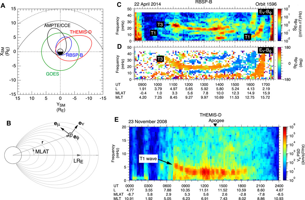
FIGURE 2. Examples of orbital dynamic spectra showing toroidal waves. (A) Selected THEMIS-D and RBSP-B orbits. Orbits of GOES and AMPTE/CCE are included as a reference. (B) Coordinate systems for spacecraft positions and the observable vector quantities used in data analysis (C,D) Cross-power spectra and cross-phase spectra of the Eν and Bϕ components measured by RBSP-B (after Takahashi and Denton, 2021). (E) Dynamic spectra of the Vϕ component measured by THEMIS-D (after Takahashi et al., 2016).
Figures 2C,D were generated from the toroidal components, δEν and δBϕ, measured by RBSP-B on the orbit shown in Figure 2A. The cross-power spectra (Figure 2C) show several toroidal harmonics, the most obvious being the fundamental (T1), second (T2), and third (T3) harmonics. The cross-phase spectra (Figure 2D), displayed only when the δEν-δBϕ coherence is higher than 0.5, also show several bands corresponding to the band structure in the cross-power spectra. The cross-phase spectra are the key to identifying the harmonic modes when many harmonics coexist or when the spectral intensity changes with time (Takahashi and Denton, 2021).
Figure 2E was generated from the δVϕ component measured by THEMIS-D on the orbit shown in Figure 2A. For an equatorially orbiting spacecraft, the velocity is a sensitive indicator of odd mode waves, which have antinodes at or near the equator. The velocity often is the best quantity for toroidal wave analysis when the electric fields measured on the same spacecraft are contaminated by spacecraft wake or charging. In this example, a strong T1 spectral line is visible. A caveat with the velocity data is that the δV spectral intensity diminishes at L < 7, where the δV is weak because of strong background B.
Included in Figure 2A are the orbit of geostationary satellites (e.g., Geostationary Operational Environmental Satellite, GOES) and an orbit of Active Magnetospheric Particle Tracer Explorers (AMPTE)/Charge Composition Explorer (CCE). The GOES satellites provide continuous B field data (not shown) at L ∼ 7. Harmonic mode identification is relatively easy with the GOES data because the magnetic latitude (MLAT) of the spacecraft does not change. Denton et al. (2016) used 12 years of data from multiple GOES satellites to develop a number of models of varying complexity for ρ at geostationary orbit. The most complicated models could determine ρ within a factor of 1.6, accounting for about two-thirds of the variance. Some GOES spacecraft carry detectors for energetic (>80 keV) protons (Rodriguez, 2014), and data from the detectors can be used to determine the frequency of oscillatory convective anisotropy induced by standing Alfvén waves (e.g., Takahashi et al., 2002). This capability remains to be utilized.
CCE had an orbital configuration intermediate between THEMIS and RBSP and was operational between 1984 and 1989. Min et al. (2013) used magnetometer data from this spacecraft to construct mass density models covering L = 4–9 and MLT = 0300–1900. The study also determined toroidal wave frequencies using GOES magnetometer data and found the frequencies to be consistent with those at CCE for L ∼ 7.
Magnetoseismology works when the driver fast mode waves for exciting toroidal waves have a wide spectral band to excite multiharmonic toroidal waves over a wide range of L. If the fast mode waves have a narrow spectrum, toroidal waves will be excited in a narrow L range and we will not be able to determine the L profile of ρ. Monochromatic fast mode waves such as wave guide modes could be excited in the magnetosphere and could produce ground magnetic pulsations with L-independent frequencies (Marin et al., 2014) while exciting magnetospheric toroidal waves on an isolated L shell. However, as Figure 2 indicates, toroidal waves (especially in the dayside magnetosphere) are usually excited over a wide frequency range in response to broadband fast mode waves generated either by dynamic pressure variations intrinsic to the solar wind (Sarris et al., 2010) or by compressional ULF waves generated in the ion foreshock (Takahashi et al., 1984). We believe that broadband fast mode waves are always present in the magnetosphere in addition to possible waveguide modes.
A number of studies used toroidal wave frequencies (fTn, n being the harmonic mode number) to find an optimal value of the α parameter appearing in Eq. 5. These studies found α values in the range 0–2, which is closer to α = 0–1 for the electron diffusive equilibrium expected in the plasmasphere rather than a collisionless distribution (α = 3–4) expected in the plasmatrough (Angerami and Carpenter, 1966; Takahashi et al., 2004). For example, Takahashi et al. (2004) obtained α ∼ 0.5 by a statistical analysis of the fTn/fT1 ratio of toroidal waves detected by the Combined Release and Radiation Effects Satellite (CRRES) spacecraft at L = 4–6 in the postnoon sector. Takahashi et al. (2015a) obtained α ∼ 0 from a detailed analysis of multiharmonic toroidal waves (n = 1–11) detected by the RBSP spacecraft during a plasmaspheric pass in the dawn sector. A statistical analysis of the fTn/fT3 ratios at RBSP in the noon sector (Takahashi and Denton, 2021) found α ∼ 2 at L = 4–6 in both the plasmasphere and the plasmatrough. Note that the α value does not need be the same between the electron density (ne) and ρ because multiple ion species with different masses and charge states, which in general have different pitch angle distributions, contribute to the latter.
In magnetoseismology, multiharmonic toroidal waves are interpreted to be superposition of independent linear waves. If the waveform is nonlinearly distorted, it will lead to regularly spaced spectral peaks and will affect α estimation. It is known that nonlinearly distorted poloidal waves produce regularly spaced spectral peaks (Higuchi et al., 1986; Takahashi et al., 2011). It is not clear whether similar distortion occurs during toroidal wave events. However, statistically determined frequency spacing between toroidal harmonics is not even, and we believe that the distortion is rare. Note that the theoretical frequencies of linear toroidal waves are evenly spaced in a dipole magnetosphere if we set α = 6 in Eq. 5 (Cummings et al., 1969; Schulz, 1996). The statistical results favoring α < 2 are an indication that nonlinear distortion is negligible.
A statistical analysis of GOES magnetometer data (Takahashi and Denton, 2007) determined the fTn/fT3 ratios at geostationary orbit (L ∼ 7) for n = 1–5 as shown in Figures 3A,B. This analysis indicated that the power-law model is only a rough approximation and that the ratios change with MLT. This finding led the authors to adopt the model given by Eq. 7. The results (Figure 3C) indicate that the mass density is peaked at the equator with the peak more pronounced at the later local times. The cause of the peak remains to be determined.
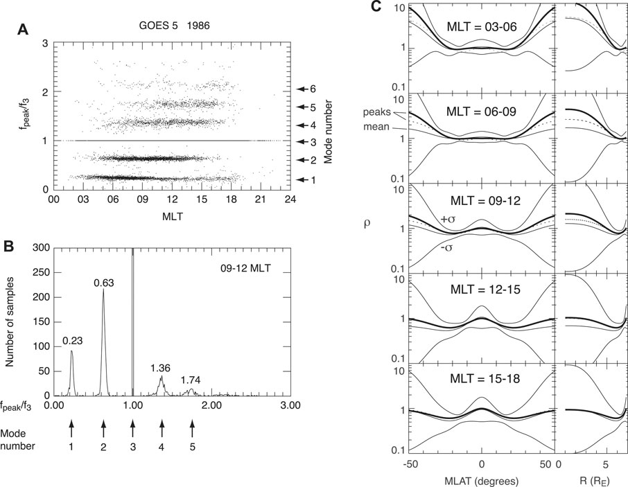
FIGURE 3. Results of GOES magnetic field data analysis (after Takahashi and Denton, 2007). (A) Frequencies at the peak of Bϕ power spectra normalized to the frequency of the third harmonic (f3). (B) Histogram of the normalized frequencies for 0900–1200 MLT. (C) Field line mass density distribution models in different MLT sectors. The mass density on the GOES magnetic field line is plotted as a function of both MLAT (left column) and geocentric distance, R, to the field line (right column).
A follow-up study (Denton et al., 2015) using the same data as those of Denton et al. (2016) developed a model for the α index at geostationary orbit,
where F10.7 is the solar extreme ultraviolet (EUV) flux index, AE is the auroral electrojet index, and MLT is in hours. Eq. 8 modeled binned values of α within a standard deviation of 0.3.
A recent study used observationally determined MLAT of the nodes of toroidal waves to select α values (Takahashi and Denton, 2021). The results shown in Figure 4 were obtained by a statistical analysis of the MLAT dependence of the amplitude and the phase of the δEν and δBϕ components measured by RBSP over a 6-month period during which the spacecraft were located on the dayside. The panels in the top and middle rows show the results for T3–T5 waves. The panels at the bottom indicate the relationship between α and the node latitudes assuming a dipole field, and the intersects of the vertical dashed lines (observed node latitudes) and the theoretical curves give the α values. This analysis indicated α ∼ 1.7 (horizontal dashed line), not far from α ∼ 2 derived in the same study using the frequencies.
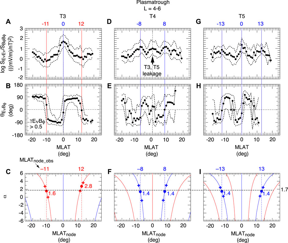
FIGURE 4. Determination of the mass density model parameter α using the node latitudes of toroidal waves observed by RBSP (after Takahashi and Denton, 2021). (A)Eν to Bϕ power ratio in the band occupied by T3 waves. The black dots are the medians, and the dashed lines indicate the upper and lower quartiles. The colored vertical lines indicate the nodes of Eν (red) and Bϕ (blue). (B)Eν-Bϕ cross phase in the T3 wave band. (C) Mass density model parameter α corresponding to the node latitudes of T3 waves (D–F) Same as (A–C) but for T4 waves B Same as (A–C) but for T5 waves.
A useful variable in magnetoseismology is the average ion mass M given by
where ρ is derived from toroidal wave frequencies and ne is sometimes available from examination of plasma wave spectra observed at spacecraft such as CRRES (Anderson et al., 1992) and RBSP (Kurth et al., 2015). The magnetospheric plasma is mostly composed of H+, He+, and O+, which means that the mass density is expressed as
with the constraint of charge neutrality
where ni and mi (i = H+, He+, or O+) are the number density and the mass of the ion species, respectively. Although we cannot determine all of the three ion number densities from the two variables ρ and ne, we can use M to infer the ion composition. The value of M should be between 1 amu (all-H+ plasma) and 16 amu (all-O+ plasma). The
Figure 5 shows the statistical properties of M samples derived using CRRES data for 1991 (solar maximum) and setting α = 0.5 (Takahashi et al., 2006). The occurrence distribution (Figure 5A) is mostly confined within 1–16 amu as expected with a median value of 3 amu. Because He+ cannot raise M to >4 amu and H+ carries the highest number density in general, it is concluded that there were substantial amounts of O+. In addition, M differs between the plasmasphere and the plasmatrough. Figure 5B shows that M ∼ 1.5 in the plasmasphere (ne > 100 cm−3) and M ∼ 3 amu in the plasmatrough (ne < 20 cm−3). Geomagnetic activity also controls M, as shown in Figure 5C, with higher values occurring when the ring current index Dst has larger magnitudes. O+ ions originate from the ionosphere, and the solar EUV intensity (F10.7) controls the density, temperature, and scale height of the O+ ions that are transported to the magnetosphere. A study that combined ρ determined using toroidal wave frequencies and ions detected by particle experiments at geosynchronous orbit (Denton et al., 2011) showed that while ρ has maximum value at solar maximum, the electron density has minimum value, so that the
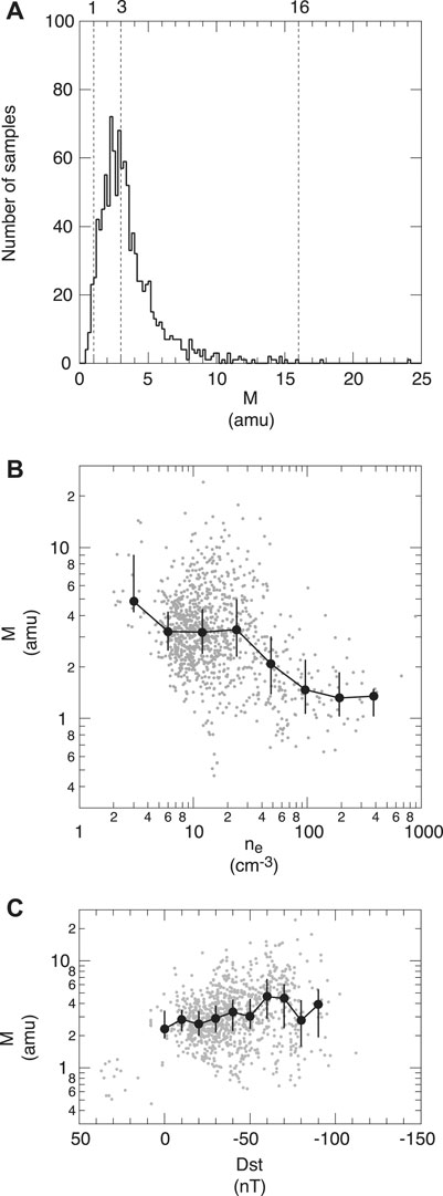
FIGURE 5. Statistical properties of the average ion mass (M) obtained using CRRES data and assuming α = 0.5 (after Takahashi et al., 2006). (A) Occurrence distribution. (B). Dependence on electron density ne. The gray dots are individual samples, the filled black circles are medians, and the vertical bars connect the upper and lower quartiles. (C) Dependence on Dst.
This
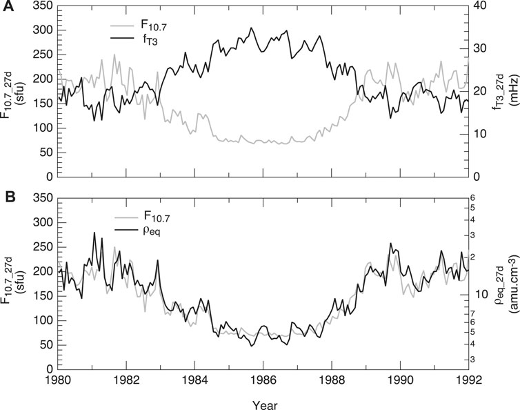
FIGURE 6. Results of a magnetoseismic study using GOES magnetometer data (after Takahashi et al., 2010). (A) Comparison of the F10.7 index and the frequency of third harmonic toroidal waves at GOES over a solar cycle. The data are 27-day averages. (B) Comparison of the F10.7 index and the mass density estimated from the wave frequency.
This equation indicates a factor of ∼4 variation of ρ over a solar cycle. Note that the GOES measurements were made at L ∼ 7 and the ρ samples were taken from the 0600–1200 MLT sector, which means that the spacecraft was mostly in the plasmatrough. A similar study using Geotail data (Takahashi et al., 2014) found that ρ at L ∼ 11 in the 0400–0800 MLT sector varied by a smaller factor of ∼2 over a solar cycle. This difference could be accounted for by the L localization of an O+-rich region, as described next.
Spatial localization of heavy ion concentration is one of the important magnetospheric phenomena that magnetoseismology can uniquely address. We show two examples. The first example (Figure 7) is taken from Takahashi et al. (2008) and shows the L profile of magnetoseismic variables for a drainage plume crossing by the CRRES spacecraft. Although the ne profile (Figure 7B) clearly indicates the distinction between the plasmatrough and the drainage plume, there is no change in fT1 (Figure 7A) at the trough-plume boundary. This difference is explained by a higher heavy ion concentration in the plasmatrough, which is evident in the L profiles of M (Figure 7C) and

FIGURE 7. Magnetoseismic variables plotted versus L for a drainage plume crossing by CRRES (after Takahashi et al., 2008). (A) Fundamental toroidal wave frequency. (B) Mass density and electron density. (C) Average ion mass. (D) Oxygen number density normalized to the electron density. The vertical bars indicate the possible range assuming (H+-O+) plasma and (He+-O+) plasma, and the open circles indicate the assumption of a fixed
The second example (Nosé et al., 2015) is shown in Figure 8. Figure 8A shows that M is elevated as high as 8 amu over an L distance ∼1 just outside the electron plasmapause located at L ∼ 3. Another study, which combined observations of Arase and RBSP (Nosé et al., 2020), demonstrated that O+ enhancement is limited in local time as well.
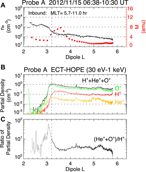
FIGURE 8. Localized heavy ion density enhancement reported in an RBSP study (after Nosé et al., 2015). (A)L profile of the electron density (black curve) and the average ion mass (red dots). (B) Number density of the H+, He+, and O+ ions obtained by taking the moment of ion fluxes measured by the HOPE instrument in the energy range 30 eV–1 keV. (C) Number density ratio between the heavy ions (He+ and O+) and H+, calculated using the data shown in panel (B).
The lower two panels of Figure 8 are included to show the difficulty in determining ρ using particle data. Figure 8B shows ion number densities calculated using data from the RBSP Helium, Oxygen, Proton, and Electron (HOPE) mass spectrometer (Funsten et al., 2013) in the energy range 30 eV—1 keV. Although HOPE has a lower energy limit at 1 eV, energies lower than 30 eV were excluded to avoid spacecraft charging effects. The HOPE-derived densities (<1 cm−3) are well below ne (>50 cm−3) determined from the plasma wave spectra, meaning that the bulk of the mass density is carried by ions with energies lower than 30 eV. Figure 8C shows that there is no indication of heavy ion enhancement in the HOPE data at the location where M is elevated. This example demonstrates that magnetoseismology captures low-energy ions that contribute to the mass density but are not measured by particle instruments.
An exception to the limitation of particle experiments occurs when the cold ion population is embedded in a fast bulk flow so that the population can be detected by particle instruments with the lower energy cutoff well above the thermal energy of the cold ions. Such flow events occur during Pc5 wave events in the outer magnetosphere (Chen, 2004; Hirahara et al., 2004; Lee and Angelopoulos, 2014) and provide opportunities to validate results from magnetoseismology.
Figure 9 shows a comparison of the ion mass density derived from ion flux measurements during a Pc5 wave event reported by Hirahara et al. (2004) and the ρ value estimated from the frequency of the wave (Takahashi et al., 2014). A 12-s snapshot of the ion phase space density (Figure 9B) exhibits three peaks at negative velocities. These peaks are attributed to the cold O+, He+, and, H+ ions that are convected at the same δE × B velocity. The velocity (>100 km/s peak to peak, Figure 9A) is higher than the background plasma convection velocity. The peaks are separated because the ion instrument (an electrostatic analyzer) does not distinguish ion species and the velocity is calculated assuming all detected ions are protons. By assigning a correct mass value to the ions contributing to each peak, it is possible to obtain the number density and mass density for each ion at each instrument duty cycle, as shown in Figure 9C. The mass density summed over the three ion species is 3.9 amu cm−3 when averaged over the time interval shown in Figure 9C. This is close to the value 3.1 amu cm−3 that is obtained from the toroidal Pc5 wave frequency. This comparison could be extended to a statistical study using many flow events detected by Geotail (e.g., Hirahara et al., 2004) and THEMIS (e.g., Lee and Angelopoulos, 2014).
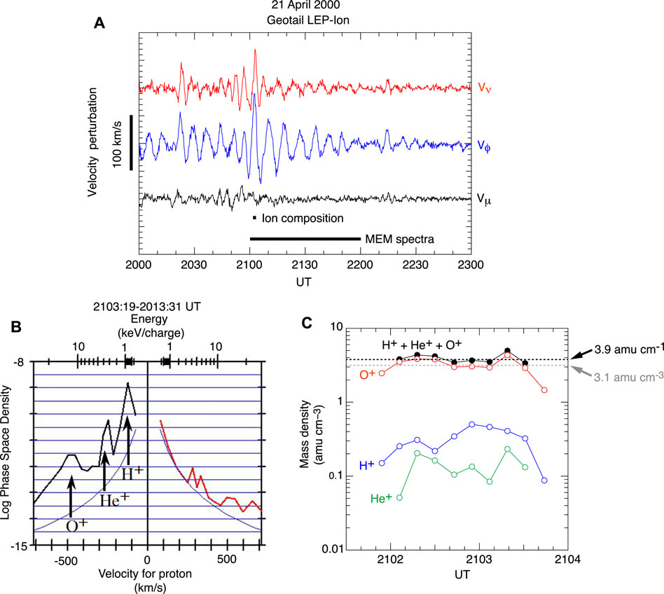
FIGURE 9. Mass density analysis using Geotail data. (A) Ion bulk velocity data indicating a Pc5 fundamental toroidal wave event (after Takahashi et al., 2014). The frequency of the Vϕ oscillation is 2.2 mHz according to the Vϕ power spectrum computed from the 1-h data segment labeled “MEM spectra.” (B) Ion phase space density snapshot obtained using ion fluxes measured in a 12-s interval during the wave event (after Hirahara et al., 2004). (C) Partial and total mass densities obtained using the phase space density for the 2.5-min interval labeled “Ion composition” in panel (A) (after Takahashi et al., 2014). The black and gray horizontal dashed lines indicate the mass densities derived from the ion data and from the Pc5 wave frequency, respectively.
A major goal of magnetoseismology is to develop a global model of ρ. Ideally, the model will reach a degree of maturity similar to that of existing models of the magnetic field (e.g., Sitnov et al., 2008), the electron density (e.g., Carpenter and Anderson, 1992; O’Brien and Moldwin, 2003; Archer et al., 2015; Liu et al., 2015), the He+ density (e.g., Gallagher et al., 2021), and the density of low energy (but excluding cold) ions (e.g., Kistler and Mouikis, 2016). Magnetoseismic studies using ground magnetometer data have made significant progress in this regard. For example, Del Corpo et al. (2020) generated a global equatorial ρ model covering L = 2.3–8 and MLT = 0600–1800 using measurements by ∼20 pairs of stations included in the European quasi-Meridional Magnetometer Array (EMMA) magnetometer network.
By contrast, there is much room for improvement in spacecraft data analysis. Spacecraft studies are invaluable because they provide information on the configuration of the background magnetic field and on ne (for derivation of M), as we stated in sections 2.3 and 3.3. Although multiyear spacecraft observations cover the entire dayside magnetosphere (see Figure 2) as well as a large portion of the magnetotail, statistical analysis of the data has been limited. Notable exceptions are GOES (e.g., Takahashi et al., 2010) and Geotail (Takahashi et al., 2014) studies covering a solar cycle and an AMPTE/CCE study covering ∼4 years (Takahashi et al., 2002; Min et al., 2013).
Figure 10 illustrates the potential of spacecraft data for the global model. Figure 10A shows the rate of detection of fundamental toroidal waves obtained in a study (Takahashi et al., 2015b) that used ion bulk velocity but did not convert the wave frequency to ρ. The waves are detected at a high rate on the dayside from L = 6 to L = 12 (spacecraft apogee). The rate becomes low on the nightside, but toroidal waves are still detected there along with Pi2 pulsations, most often after substorm onsets (Takahashi et al., 1988; Takahashi et al., 2018) and when ULF waves generated in the ion foreshock penetrate deep into the magnetosphere (Takahashi et al., 2020). The presence of substorm-related toroidal waves is evident in Figure 10B as a region of large δVϕ amplitudes in the premidnight sector.
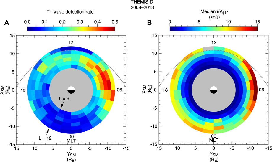
FIGURE 10. L-MLT maps of fundamental toroidal waves detected in the ion bulk velocity measured by THEMIS-D (after Takahashi et al., 2015b). The dotted line is a model magnetopause. (A) Rate of detection. (B) Median amplitude.
Figure 11 shows a magnetoseismic study using toroidal waves detected by the Arase spacecraft in the midnight sector away from the magnetic equator. The waves were detected after Pi2 onsets on the ground. An RBSP spacecraft located near the magnetic equator detected compressional oscillations, which can be cavity mode oscillations. Because the AE index had moderate values (<200 nT) during the wave event in this example, we expect that nightside Pi2 waves and toroidal waves are commonly excited and can be easily detected off the magnetic equator in association with small substorms or other minor disturbances in the magnetotail. Because it appears difficult to determine nightside toroidal wave frequencies with ground magnetometers (Takahashi et al., 2020), we expect that a model derived using spacecraft data will perform better on the nightside than models derived using only ground data.
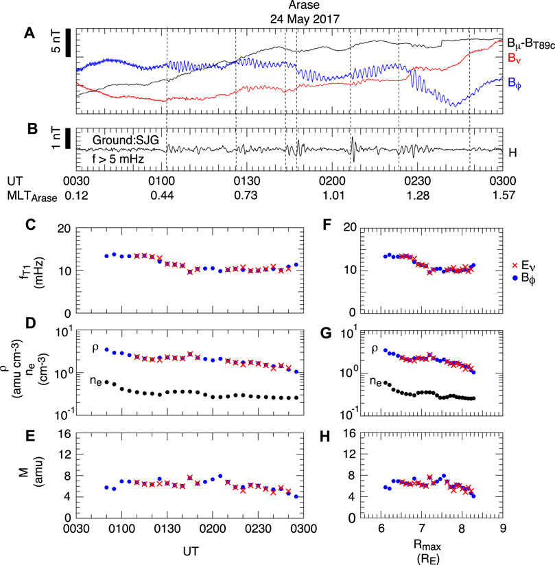
FIGURE 11. Magnetoseismic analysis of toroidal waves detected by the Arase spacecraft in the midnight sector (after Takahashi et al., 2018). (A) Magnetic field components in a magnetic-field-aligned coordinate system based on the T89c magnetic field model (Tsyganenko, 1989). Fundamental toroidal waves are visible in the Bϕ component. (B) High-pass-filtered ground magnetic field H component at San Juan. The dashed vertical lines indicate Pi2 onsets. (C) Frequency of the fundamental toroidal waves. The color indicates the source field component. (D) Mass density derived from the wave frequency and the electron density determined from plasma wave spectra. (E) Average ion mass. (F–H) Same quantities as in (C–E) but plotted as a function of the maximum geocentric distance to the model field line.
We discuss limitations, unresolved issues, and areas in need of improvements in magnetoseismic studies.
To relate observed fTn to ρ, standing wave equations (e.g., Eq. 3) are solved usually assuming perfect reflection, corresponding to infinitely high height-integrated Pedersen conductivity ΣP, at a fixed ionospheric altitude. In reality, the ionosphere has a finite thickness and the conductivity is finite. We discuss whether the assumption is appropriate.
The assumption of a thin ionosphere is justified because the thickness of the ionosphere (∼300 km) is much shorter than the hemispheric length (>15,000 km) of magnetic field lines at L > 2.5, where reliable measurements of wave frequency can be made by spacecraft on low-inclination elliptical orbits (Takahashi and Denton, 2021). On these field lines, the Alfvén wave velocity at the ionospheric altitude is usually higher than near the equator, making the Alfvén wave travel time through the ionosphere much smaller than that through the region above the ionosphere. This means that the details of wave propagation through the ionosphere do not affect fTn in any significant way.
There are questions about the ΣP. This conductivity, which controls the damping rate of toroidal waves, depends on solar illumination and particle precipitation from the magnetosphere, both of which are a function of latitude and local time as well. According to numerical studies of the ΣP dependence of fTn (e.g., Newton et al., 1978), the frequency is very close to that of perfectly reflected waves when ΣP is higher than a critical value (denoted ΣP0) corresponding to impedance matching between the ionosphere and the waves. At locations where solar illumination is low or zero, the conductivity may become lower than ΣP0, leading to strong damping of the waves or transition of the waves to free-end modes with lower fTn values (Newton et al., 1978). If one end of a field line is anchored to the sunlit part of the ionosphere and the other is anchored to the dark part, theory predicts that the usual half-wave T1 modes turn to quarter-wave modes (Allan and Knox, 1979). Quarter-wave modes at L ∼ 3 have been detected at the dawn terminator by ground magnetometers (Obana et al., 2008). If the quarter-wave and half-wave modes are not distinguished, it will lead to a serious error in ρ. Investigation of the quarter-wave modes in space remains to be done.
Yet nightside multiharmonic toroidal waves are readily detected by spacecraft and exhibit properties consistent with high ionospheric reflection even when observed within the plasmasphere (Takahashi et al., 2020), where precipitation is not expected to be high enough to maintain high ΣP according to empirical ionospheric density models (e.g., Wallis and Budzinski, 1981). This poses an interesting question of what elevates the ionospheric conductivity and whether high conductivity occurs commonly to make nightside magnetoseismology possible. One interesting possibility is that ULF waves themselves enhance ionospheric conductivity through modulation of electron precipitation (Jaynes et al., 2015). Wang et al. (2020) reported strong modulation of the conductivity by storm-time compressional Pc5 waves. Whether similar precipitation modulations occur during less geomagnetically active periods remains to be understood.
Magnetoseismology based on spacecraft data poses challenges that are not encountered with ground magnetometer data. First, wave frequency and amplitude seen from a moving spacecraft change continuously even if the waves do not have intrinsic temporal variations. The L dependence is particularly important. For example, fT1 within the plasmasphere decreases from ∼20 mHz at L ∼ 2.5 to ∼ 5 mHz at L ∼ 4 (Takahashi and Anderson, 1992; Takahashi and Denton, 2021). As spacecraft such as THEMIS and RBSP move rapidly in the radial direction in the L < 4 region, it is necessary to choose a proper time window for spectral analysis so that the spatial variation of the frequency is resolved. The studies cited in this paper used data windows of a fixed length, although Min et al. (2013) introduced a variable data sampling rate to handle the spatial variation of fTn at L > 4.
The inferred ρ is proportional to the inverse square of the observed Alfvén frequency (Eq. 4), and we usually consider that frequency to be the largest source of error. The uncertainty of the frequency can be determined from the frequency spectrum (Denton et al., 2001). Other sources of error are the magnetic field at the spacecraft location and the field line dependence of the magnetic field and mass density. In most cases, the magnetic field at the spacecraft location is known. In the best case, the measurement is near the magnetic equator, which is the region that most greatly affects the Alfvén frequency. The field line dependence of the magnetic field and mass density does have some effect on the inferred value of the mass density, but that effect is usually smaller than the uncertainty associated with the frequency. If, on the other hand, the field line is mapped from low-Earth orbit or the ground, or if the spacecraft is in the outer magnetosphere (particularly at L greater than 8), there can be significant uncertainties for the magnetic field and/or field line mapping (Takahashi et al., 2006; Takahashi et al., 2010).
Another issue related to spacecraft motion is frequency shift. The shift occurs because toroidal waves have a finite L width (FLR width) within which the wave phase changes by 180°. In regions where the wave frequency decreases with L (e.g., the plasmasphere), the wave phase is delayed from lower L to higher L. This spatial phase structure leads to frequency downshift (upshift) at spacecraft moving to higher (lower) L by an amount given by
where vL is the equatorial L-crossing speed and ɛ is the equatorial semiwidth of FLR (Vellante et al., 2004; Heilig et al., 2013). The frequency shift is found to be significant (20–25 mHz for T1 waves at L < 2.4) when observations are compared between the polar-orbiting Challenging Minisatellite Payload (CHAMP) spacecraft and ground magnetometers (Heilig et al., 2013).
At equatorial-orbiting spacecraft, Δf is smaller but may not be negligible. As an example, we evaluate Δf at RBSP. For the spacecraft, vL has a peak value of ∼ 5 km/s at L = 1.5, decreases to ∼3 km/s at L = 3, and becomes zero at L ∼ 6 (apogee). If we assume ɛ = 200 km, which was the case for a 14 mHz toroidal wave at L ∼ 5 (Takahashi et al., 2015a), we get Δf ∼ 2 mHz at L = 3. This frequency shift is ∼ 10% of fT1 (∼20 mHz) at L = 3 (Takahashi and Anderson, 1992) and translates to a ρ error of ∼ 20% (see Eq. 4). This error can explain why M derived from fTn observed on outbound RBSP passes is higher at L < 3 (large vL) than at L > 3 (small vL) (Vellante et al., 2021). Evaluation of ɛ at various radial distances and local times is necessary to improve our understanding of Δf.
Finally, fully automated methods are lacking to determine fTn in space. As a result, only a small fraction of satellite data that are potentially useful has been used in magnetoseismic studies. The procedure is the easiest for T1 waves detected in the outer magnetosphere using plasma bulk flow data (Takahashi et al., 2014; Takahashi et al.,2016). Regular oscillations in the azimuthal component of the velocity are almost always associated with T1 waves, and not much manual work is required to distinguish them from other waves. Processing magnetic field data from geostationary orbits is also relatively easy with the spacecraft staying at a fixed L leading to a stable appearance of the spectral intensity of each harmonic. Processing data from elliptically orbiting spacecraft is the most difficult because of the rapid change of spacecraft radial distance, crossing of the nodes, and the presence of waves other than toroidal waves.
It appears that at some stage we need to introduce a technique such as neural network analysis to automate the interpretation of the wave spectra. The main required capability of the technique is to reject spectral peaks that do not result from toroidal waves. In this regard, we note that the quality of E and B data from spacecraft depends on the mode of sensor operation, location and attitude of the spacecraft, and the plasma environment (for E). In addition, spacecraft spin and nutation of sensor booms introduce noise lines at fixed frequencies but with varying amplitudes. Some of the spectral peaks caused by these artifacts are predictable, but they can overlap fTn as spacecraft move in L. Also, there are unpredictable peaks that originate from ULF waves that are not toroidal waves. An automated method to determine electron density has been developed by applying a neural-network algorithm to plasma wave spectrograms (Zhelavskaya et al., 2016), and we may design a similar algorithm for fTn.
Although significant progress has been made modeling the mass density and field line dependence at geostationary orbit (e.g., Denton et al., 2015; Denton et al.,2016), further work needs to be done to develop an accurate radially dependent model. Neural network analysis might also be helpful here, as it has been for modeling electron density (Chu et al., 2017).
Another need is for event-specific mass density field line dependence. With the possible exception of the event studied by Denton et al. (2009), which had a particularly accurate set of frequencies, significant uncertainty in the observed Alfvén frequencies has precluded an accurate determination of event-specific field line dependence. So, most studies have been statistical (e.g., Denton et al., 2006, Denton et al., 2015; Takahashi and Denton, 2007). Perhaps the mode structure technique described in subsection 3.2 will enable event-specific determination of the field line dependence, but that is yet to be shown.
Finally, we note that magnetoseismology belongs to a family of techniques to probe the magnetospheric plasma structure without using in situ particle measurements. Other techniques include EUV imaging of the plasmasphere (Sandel et al., 2003), energetic neutral atom remote (ENA) sensing of energetic ions (Roelof et al., 1985; Brandt et al., 2005), estimation of ne using whistler waves (Carpenter and Smith, 1964; Park, 1974), spacecraft potential (Pedersen et al., 1984; Archer et al., 2015), or plasma wave spectra (upper hybrid resonance) (Mosier et al., 1973; Moldwin et al., 2002; Thomas et al., 2021). These indirect techniques are complementary to each other. For example, the global imaging techniques are capable of taking snapshots of plasma structures, which cannot be obtained using the magnetoseismic or ne techniques unless we have a large number of measurement points. The magnetoseismic and ne techniques provide the total densities, whereas ENA images provide information on the density of energetic ions (>10 keV). Improvement of magnetoseismic techniques and associated datasets is much desired to enhance the synergy of different density-related techniques.
Toroidal waves detected by spacecraft are a valuable resource from which the magnetospheric mass density (ρ) is estimated. Some spacecraft also provide electron density (ne) data, and from the average ion mass M (= ρ/ne), we can infer the ion composition and the presence of heavy ions (i.e., O+). We reviewed progress made mainly in the past decade. The basic techniques to identify wave frequencies and convert them to the mass density are well established. The challenge is to apply the techniques to data from various spacecraft in an efficient way to develop global ρ and M models that have dependencies on position, solar activity, and solar wind and geomagnetic conditions.
KT and RD jointly prepared this review paper, based mostly on their own research published in scientific journals.
National Science Foundation, Award Number 1840970. National Aeronautics and Space Administration, Award Number 80NSSC20K1446 and Award Number 80NSSC21K0453.
The authors declare that the research was conducted in the absence of any commercial or financial relationships that could be construed as a potential conflict of interest.
All claims expressed in this article are solely those of the authors and do not necessarily represent those of their affiliated organizations, or those of the publisher, the editors and the reviewers. Any product that may be evaluated in this article, or claim that may be made by its manufacturer, is not guaranteed or endorsed by the publisher.
This paper is an expanded version of a presentation made at the 2020 meeting entitled “The Impact of the Cold Plasma Populations in the Earth’s Magnetosphere.” The authors thank Gian Luca Delzanno and Joseph E. Borovsky for organizing the meeting and encouraging preparation of this manuscript.
Allan, W., and Knox, F. B. (1979). The Effect of Finite Ionosphere Conductivities on Axisymmetric Toroidal Alfvén Wave Resonances. Planet. Space Sci. 27, 939–950. doi:10.1016/0032-0633(79)90024-2
Allan, W., White, S. P., and Poulter, E. M. (1986). Impulse-excited Hydromagnetic Cavity and Field-Line Resonances in the Magnetosphere. Planet. Space Sci. 34, 371–385. doi:10.1016/0032-0633(86)90144-3
Anderson, B. J., Engebretson, M. J., Rounds, S. P., Zanetti, L. J., and Potemra, T. A. (1990). A Statistical Study of Pc 3–5 Pulsations Observed by the AMPTE/CCE Magnetic fields experiment, 1. Occurrence Distributions. J. Geophys. Res. 95, 10495–10523. doi:10.1029/JA095iA07p10495
Anderson, R. R., Gurnett, D. A., and Odem, D. L. (1992). The CRRES Plasma Wave experiment. J. Spacecraft Rockets 29, 570–574. doi:10.2514/3.25501
Angerami, J. J., and Carpenter, D. L. (1966). Whistler Studies of the Plasmapause in the Magnetosphere: 2. Electron Density and Total Tube Electron Content Near the Knee in Magnetospheric Ionization. J. Geophys. Res. 71, 711–725. doi:10.1029/JZ071i003p00711
Archer, M. O., Hartinger, M. D., Walsh, B. M., Plaschke, F., and Angelopoulos, V. (2015). Frequency Variability of Standing Alfvén Waves Excited by Fast Mode Resonances in the Outer Magnetosphere. Geophys. Res. Lett. 42, 10150–10159. doi:10.1002/2015gl066683
Arthur, C. W., and McPherron, R. L. (1981). The Statistical Character of Pc 4 Magnetic Pulsations at Synchronous Orbit. J. Geophys. Res. 86, 1325. doi:10.1029/JA086iA03p01325
Brandt, P. C., Mitchell, D. G., Roelof, E. C., Krimigis, S. M., Paranicas, C. P., Mauk, B. H., et al. (2005). ENA Imaging: Seeing the Invisible. Johns Hopkins APL Tech. Dig. 26, 143–155.
Carpenter, D. L., and Anderson, R. R. (1992). An ISEE/whistler Model of Equatorial Electron Density in the Magnetosphere. J. Geophys. Res. Space Phys. 97, 1097–1108. doi:10.1029/91ja01548
Carpenter, D. L., and Smith, R. L. (1964). Whistler Measurements of Electron Density in the Magnetosphere. Rev. Geophys. 2. doi:10.1029/RG002i003p00415
Chen, L., and Hasegawa, A. (1974). A Theory of Long-Period Magnetic Pulsations: 1. Steady State Excitation of Field Line Resonance. J. Geophys. Res. 79, 1024–1032. doi:10.1029/JA079i007p01024
Chen, S. H. (2004). Dayside Flow Bursts in the Earth’s Outer Magnetosphere. J. Geophys. Res. 109. doi:10.1029/2003ja010007
Chi, P. J., and Russell, C. T. (2005). Travel-time Magnetoseismology: Magnetospheric Sounding by Timing the Tremors in Space. Geophys. Res. Lett. 32, L18108. doi:10.1029/2005gl023441
Chu, X., Bortnik, J., Li, W., Ma, Q., Denton, R., Yue, C., et al. (2017). A Neural Network Model of Three-Dimensional Dynamic Electron Density in the Inner Magnetosphere. J. Geophys. Res. Space Phys. 122, 9183–9197. doi:10.1002/2017ja024464
Claudepierre, S. G., Hudson, M. K., Lotko, W., Lyon, J. G., and Denton, R. E. (2010). Solar Wind Driving of Magnetospheric ULF Waves: Field Line Resonances Driven by Dynamic Pressure Fluctuations. J. Geophys. Res. Space Phys. 115. doi:10.1029/2010ja015399
Craven, P. D., Gallagher, D. L., and Comfort, R. H. (1997). Relative Concentration of He+ in the Inner Magnetosphere as Observed by the DE 1 Retarding Ion Mass Spectrometer. J. Geophys. Res. Space Phys. 102, 2279–2289. doi:10.1029/96ja02176
Cummings, W. D., O’Sullivan, R. J., and Coleman, P. J. (1969). Standing Alfvén Waves in the Magnetosphere. J. Geophys. Res. 74, 778–793. doi:10.1029/JA074i003p00778
Del Corpo, A., Vellante, M., Heilig, B., Pietropaolo, E., Reda, J., and Lichtenberger, J. (2020). An Empirical Model for the Dayside Magnetospheric Plasma Mass Density Derived from EMMA Magnetometer Network Observations. J. Geophys. Res. Space Phys. 125. doi:10.1029/2019ja027381
Denton, R. E., Décréau, P., Engebretson, M. J., Darrouzet, F., Posch, J. L., Mouikis, C., et al. (2009). Field Line Distribution of Density at L = 4.8 Inferred from Observations by CLUSTER. Ann. Geophysicae 27, 705–724. doi:10.5194/angeo-27-705-2009
Denton, R. E., Lessard, M. R., Anderson, R., Miftakhova, E. G., and Hughes, J. W. (2001). Determining the Mass Density along Magnetic Field Lines from Toroidal Eigenfrequencies: Polynomial Expansion Applied to CRRES Data. J. Geophys. Res. Space Phys. 106, 29915–29924. doi:10.1029/2001ja000204
Denton, R. E. (2006). “Magneto-seismology Using Spacecraft Observations,” in Magnetospheric ULF Waves: Synthesis and New Directions. Editors K. Takahashi, P. J. Chi, R. E. Denton, and R. L. Lysak (Washington DC: AGU). 307–317.
Denton, R. E. (2003). Radial Localization of Magnetospheric Guided Poloidal Pc 4–5 Waves. J. Geophys. Res. 108, 1105. doi:10.1029/2002ja009679
Denton, R. E., Takahashi, K., Amoh, J., and Singer, H. J. (2016). Mass Density at Geostationary Orbit and Apparent Mass Refilling. J. Geophys. Res. Space Phys. 121, 2962–2975. doi:10.1002/2015ja022167
Denton, R. E., Takahashi, K., Anderson, R. R., and Wuest, M. P. (2004). Magnetospheric Toroidal Alfvén Wave Harmonics and the Field Line Distribution of Mass Density. J. Geophys. Res. 109, A06202. doi:10.1029/2003ja010201
Denton, R. E., Takahashi, K., Galkin, I. A., Nsumei, P. A., Huang, X., Reinisch, B. W., et al. (2006). Distribution of Density along Magnetospheric Field Lines. J. Geophys. Res. 111, A04213. doi:10.1029/2005ja011414
Denton, R. E., Takahashi, K., Lee, J., Zeitler, C. K., Wimer, N. T., Litscher, L. E., et al. (2015). Field Line Distribution of Mass Density at Geostationary Orbit. J. Geophys. Res. Space Phys. 120, 4409–4422. doi:10.1002/2014ja020810
Denton, R. E., Thomsen, M. F., Takahashi, K., Anderson, R. R., and Singer, H. J. (2011). Solar Cycle Dependence of Bulk Ion Composition at Geosynchronous Orbit. J. Geophys. Res. Space Phys. 116, A03212. doi:10.1029/2010ja016027
Dungey, D. W. (1954). Electrodynamics of the Outer Atmosphere. PA: Scientific Report, Ionosphere Research Laboratory, Pennsylvania State University, University Park, 69.
Funsten, H. O., Skoug, R. M., Guthrie, A. A., MacDonald, E. A., Baldonado, J. R., Harper, R. W., et al. (2013). Helium, Oxygen, Proton, and Electron (HOPE) Mass Spectrometer for the Radiation Belt Storm Probes mission. Space Sci. Rev. 179, 423–484. doi:10.1007/s11214-013-9968-7
Gallagher, D. L., Comfort, R. H., Katus, R. M., Sandel, B. R., Fung, S. F., and Adrian, M. L. (2021). The Breathing Plasmasphere: Erosion and Refilling. J. Geophys. Res. Space Phys. 126. doi:10.1029/2020ja028727
Heilig, B., Sutcliffe, P. R., Ndiitwani, D. C., and Collier, A. B. (2013). Statistical Study of Geomagnetic Field Line Resonances Observed by CHAMP and on the Ground. J. Geophys. Res. Space Phys. 118, 1934–1947. doi:10.1002/jgra.50215
Higuchi, T., Kokubun, S., and Ohtani, S. (1986). Harmonic Structure of Compressional Pc5 Pulsations at Synchronous Orbit. Geophys. Res. Lett. 13, 1101–1104. doi:10.1029/GL013i011p01101
Hirahara, M., Seki, K., Saito, Y., and Mukai, T. (2004). Periodic Emergence of Multicomposition Cold Ions Modulated by Geomagnetic Field Line Oscillations in the Near-Earth Magnetosphere. J. Geophys. Res. Space Phys. 109, A0321. doi:10.1029/2003ja010141
Hughes, W. J., and Southwood, D. J. (1976). The Screening of Micropulsation Signals by the Atmosphere and Ionosphere. J. Geophys. Res. 81, 3234–3240. doi:10.1029/JA081i019p03234
Jaynes, A. N., Lessard, M. R., Takahashi, K., Ali, A. F., Malaspina, D. M., Michell, R. G., et al. (2015). Correlated Pc4–5 ULF Waves, Whistler-Mode Chorus, and Pulsating aurora Observed by the Van Allen Probes and Ground-Based Systems. J. Geophys. Res. Space Phys. 120, 8749–8761. doi:10.1002/2015ja021380
Kistler, L. M., and Mouikis, C. G. (2016). The Inner Magnetosphere Ion Composition and Local Time Distribution over a Solar Cycle. J. Geophys. Res. Space Phys. 121, 2009–2032. doi:10.1002/2015ja021883
Krall, J., Huba, J. D., and Fedder, J. A. (2008). Simulation of Field-Aligned H+ and He+ Dynamics during Late-Stage Plasmasphere Refilling. Ann. Geophysicae 26, 1507–1516. doi:10.5194/angeo-26-1507-2008
Kurth, W. S., De Pascuale, S., Faden, J. B., Kletzing, C. A., Hospodarsky, G. B., Thaller, S., et al. (2015). Electron Densities Inferred from Plasma Wave Spectra Obtained by the Waves Instrument on Van Allen Probes. J. Geophys. Res. Space Phys. 120, 904–914. doi:10.1002/2014JA020857
Lee, D.-H., and Lysak, R. L. (1989). Magnetospheric ULF Wave Coupling in the Dipole Model: The Impulsive Excitation. J. Geophys. Res. 94, 17097–17103. doi:10.1029/JA094iA12p17097
Lee, D. H., Lysak, R. L., and Song, Y. (2000). Field Line Resonances in a Nonaxisymmetric Magnetic Field. J. Geophys. Res. Space Phys. 105, 10703–10711. doi:10.1029/1999ja000295
Lee, J. H., and Angelopoulos, V. (2014). On the Presence and Properties of Cold Ions Near Earth’s Equatorial Magnetosphere. J. Geophys. Res. Space Phys. 119, 1749–1770. doi:10.1002/2013ja019305
Liu, W., Cao, J. B., Li, X., Sarris, T. E., Zong, Q. G., Hartinger, M., et al. (2013). Poloidal ULF Wave Observed in the Plasmasphere Boundary Layer. J. Geophys. Res. Space Phys. 118, 4298–4307. doi:10.1002/jgra.50427
Liu, X., Liu, W., Cao, J. B., Fu, H. S., Yu, J., and Li, X. (2015). Dynamic Plasmapause Model Based on THEMIS Measurements. J. Geophys. Res. Space Phys. 120, 10543–10556. doi:10.1002/2015ja021801
Marin, J., Pilipenko, V., Kozyreva, O., Stepanova, M., Engebretson, M., Vega, P., et al. (2014). Global Pc5 Pulsations during strong Magnetic Storms: Excitation Mechanisms and Equatorward Expansion. Ann. Geophysicae 32, 319–331. doi:10.5194/angeo-32-319-2014
Menk, F. W., and Waters, C. L. (2013). Magnetoseismology. Weinheim: Wiley VCH. doi:10.1002/9783527652051
Min, K., Bortnik, J., Denton, R. E., Takahashi, K., Lee, J., and Singer, H. J. (2013). Quiet Time Equatorial Mass Density Distribution Derived from AMPTE/CCE and GOES Using the Magnetoseismology Technique. J. Geophys. Res. Space Phys. 118, 6090–6105. doi:10.1002/jgra.50563
Moldwin, M. B., Downward, L., Rassoul, H. K., Amin, R., and Anderson, R. R. (2002). A New Model of the Location of the Plasmapause: CRRES Results. J. Geophys. Res. 107, 1339. doi:10.1029/2001ja009211
Mosier, S. R., Kaiser, M. L., and Brown, L. W. (1973). Observations of Noise Bands Associated with the Upper Hybrid Resonance by the Imp 6 Radio Astronomy Experiment. J. Geophys. Res. 78, 1673–1679. doi:10.1029/JA078i010p01673
Newton, R. S., Southwood, D. J., and Hughes, W. J. (1978). Damping of Geomagnetic Pulsations by the Ionosphere. Planet. Space Sci. 26, 201–209. doi:10.1016/0032-0633(78)90085-5
Nosé, M., Matsuoka, A., Kumamoto, A., Kasahara, Y., Teramoto, M., Kurita, S., et al. (2020). Oxygen Torus and its Coincidence with EMIC Wave in the Deep Inner Magnetosphere: Van Allen Probe B and Arase Observations. Earth Planets Space 72, 111. doi:10.1186/s40623-020-01235-w
Nosé, M., Oimatsu, S., Keika, K., Kletzing, C. A., Kurth, W. S., Pascuale, S. D., et al. (2015). Formation of the Oxygen Torus in the Inner Magnetosphere: Van Allen Probes Observations. J. Geophys. Res. Space Phys. 120, 1182–1196. doi:10.1002/2014ja020593
Obana, Y., Menk, F. W., Sciffer, M. D., and Waters, C. L. (2008). Quarter-wave Modes of Standing Alfvén Waves Detected by Cross-phase Analysis. J. Geophys. Res. Space Phys. 113. doi:10.1029/2007ja012917
Obayashi, T., and Jacobs, J. A. (1958). Geomagnetic Pulsations and the Earth’s Outer Atmosphere. Geophys. J. Int. 1, 53–63. doi:10.1111/j.1365-246X.1958.tb00034.x
O’Brien, T. P., and Moldwin, M. B. (2003). Empirical Plasmapause Models from Magnetic Indices. Geophys. Res. Lett. 30, 1152. doi:10.1029/2002gl016007
Park, C. G. (1974). Some Features of Plasma Distribution in the Plasmasphere Deduced from Antarctic Whistlers. J. Geophys. Res. 79, 169–173. doi:10.1029/JA079i001p00169
Pedersen, A., Cattell, C. A., Mozer, F., Falthammar, C.-G., Lindqvist, P.-A., Formisano, V., et al. (1984). Quasistatic Electric Field Measurements with Spherical Double Probes on the GEOS and ISEE Satellites. Space Sci. Rev. 37, 269–312. doi:10.1007/BF00226365
Radoski, H. R., and Carovillano, R. L. (1966). Axisymmetric Plasmasphere resonances:Toroidal Mode. Phys. Fluids 9, 285–291. doi:10.1063/1.1761671
Radoski, H. R. (1967). Highly Asymmetric MHD Resonances: The Guided Poloidal Mode. J. Geophys. Res. 72, 4026–4027. doi:10.1029/JZ072i015p04026
Rankin, R., Kabin, K., and Marchand, R. (2006). Alfvénic Field Line Resonances in Arbitrary Magnetic Field Topology. Adv. Space Res. 38, 1720–1729. doi:10.1016/j.asr.2005.09.034
Rodriguez, J. V. (2014). GOES 13–15 MAGE/PD Pitch Angle Algorithm Theoretical Basis Document. Version 1.0. Silver Spring, MD: Report, National Oceanic and Atmospheric Administration/National Environmental Satellite, Data, and Information Service/National Geophysical Data Center.
Roelof, E. C., Mitchell, D. G., and Williams, D. J. (1985). Energetic Neutral Atoms (E ∼50 Kev) from the Ring Current: IMP 7/8 and ISEE 1. J. Geophys. Res. 90. doi:10.1029/JA090iA11p10991
Sandel, B. R., Goldstein, J., Gallagher, D. L., and Spasojevic, M. (2003). Extreme Ultraviolet Imager Observations of the Structure and Dynamics of the Plasmasphere. Space Sci. Rev. 109, 25–46. doi:10.1023/B:SPAC.0000007511.47727.5b
Sarris, T. E., Liu, W., Li, X., Kabin, K., Talaat, E. R., Rankin, R., et al. (2010). THEMIS Observations of the Spatial Extent and Pressure-Pulse Excitation of Field Line Resonances. Geophys. Res. Lett. 37, L15104. doi:10.1029/2010gl044125
Schulz, M. (1996). Eigenfrequencies of Geomagnetic Field Lines and Implications for Plasma-Density Modeling. J. Geophys. Res. Space Phys. 101, 17385–17397. doi:10.1029/95ja03727
Singer, H. J., Southwood, D. J., Walker, R. J., and Kivelson, M. G. (1981). Alfven Wave Resonances in a Realistic Magnetospheric Magnetic Field Geometry. J. Geophys. Res. Space Phys. 86, 4589–4596. doi:10.1029/JA086iA06p04589
Sitnov, M. I., Tsyganenko, N. A., Ukhorskiy, A. Y., and Brandt, P. C. (2008). Dynamical Data-Based Modeling of the Storm-Time Geomagnetic Field with Enhanced Spatial Resolution. J. Geophys. Res. 113, A07218. doi:10.1029/2007JA013003
Takahashi, K., and Anderson, B. J. (1992). Distribution of ULF Energy (F < 80 mHz) in the Inner Magnetosphere: A Statistical Analysis of AMPTE CCE Magnetic Field Data. J. Geophys. Res. 97, 10751. doi:10.1029/92ja00328
Takahashi, K., Denton, R. E., Anderson, R. R., and Hughes, W. J. (2004). Frequencies of Standing Alfvén Wave Harmonics and Their Implication for Plasma Mass Distribution along Geomagnetic Field Lines: Statistical Analysis of CRRES Data. J. Geophys. Res. Space Phys. 109, A08202. doi:10.1029/2003ja010345
Takahashi, K., Denton, R. E., Anderson, R. R., and Hughes, W. J. (2006). Mass Density Inferred from Toroidal Wave Frequencies and its Comparison to Electron Density. J. Geophys. Res. Space Phys. 111, A01201. doi:10.1029/2005ja011286
Takahashi, K., Denton, R. E., and Gallagher, D. (2002). Toroidal Wave Frequency at L = 6–10: Active Magnetospheric Particle Tracer Explorers/CCE Observations and Comparison with Theoretical Model. J. Geophys. Res. Space Phys. 107. SMP 2–1–SMP 2–14. doi:10.1029/2001ja000197
Takahashi, K., Denton, R. E., Hirahara, M., Min, K., Ohtani, S.-i., and Sanchez, E. (2014). Solar Cycle Variation of Plasma Mass Density in the Outer Magnetosphere: Magnetoseismic Analysis of Toroidal Standing Alfvén Waves Detected by Geotail. J. Geophys. Res. Space Phys. 119, 8338–8356. doi:10.1002/2014ja020274
Takahashi, K., Denton, R. E., Kurth, W., Kletzing, C., Wygant, J., Bonnell, J., et al. (2015a). Externally Driven Plasmaspheric ULF Waves Observed by the Van Allen Probes. J. Geophys. Res. Space Phys. 120, 526–552. doi:10.1002/2014ja020373
Takahashi, K., and Denton, R. E. (2007). Magnetospheric Seismology Using Multiharmonic Toroidal Waves Observed at Geosynchronous Orbit. J. Geophys. Res. 112. doi:10.1029/2006ja011709
Takahashi, K., Denton, R. E., Motoba, T., Matsuoka, A., Kasaba, Y., Kasahara, Y., et al. (2018). Impulsively Excited Nightside Ultralow Frequency Waves Simultaneously Observed on and off the Magnetic Equator. Geophys. Res. Lett. 45, 7918–7926. doi:10.1029/2018gl078731
Takahashi, K., and Denton, R. E. (2021). Nodal Structure of Toroidal Standing Alfvén Waves and its Implication for Field Line Mass Density Distribution. J. Geophys. Res. Space Phys. 126. doi:10.1029/2020ja028981
Takahashi, K., Denton, R. E., and Singer, H. J. (2010). Solar Cycle Variation of Geosynchronous Plasma Mass Density Derived from the Frequency of Standing Alfvén Waves. J. Geophys. Res. Space Phys. 115, A07207. doi:10.1029/2009ja015243
Takahashi, K., Glassmeier, K. H., Angelopoulos, V., Bonnell, J., Nishimura, Y., Singer, H. J., et al. (2011). Multisatellite Observations of a Giant Pulsation Event. J. Geophys. Research-Space Phys. 116. doi:10.1029/2011ja016955
Takahashi, K., Hartinger, M. D., Angelopoulos, V., and Glassmeier, K.-H. (2015b). A Statistical Study of Fundamental Toroidal Mode Standing Alfvén Waves Using THEMIS Ion Bulk Velocity Data. J. Geophys. Res. Space Phys. 120, 6474–6495. doi:10.1002/2015ja021207
Takahashi, K., Kokubun, S., Sakurai, T., McEntire, R. W., Potemra, T. A., and Lopez, R. E. (1988). AMPTE/CCE Observations of Substorm-Associated Standing Alfvén Waves in the Midnight Sector. Geophys. Res. Lett. 15, 1287–1290. doi:10.1029/GL015i011p01287
Takahashi, K., Lee, D.-H., Merkin, V. G., Lyon, J. G., and Hartinger, M. D. (2016). On the Origin of the Dawn-Dusk Asymmetry of Toroidal Pc5 Waves. J. Geophys. Res. Space Phys. 121, 9632–9650. doi:10.1002/2016ja023009
Takahashi, K., McPherron, R. L., and Hughes, W. J. (1984). Multispacecraft Observations of the Harmonic Structure of Pc 3-4 Magnetic Pulsations. J. Geophys. Res. 89, 6758–6774. doi:10.1029/JA089iA08p06758
Takahashi, K., and McPherron, R. L. (1984). Standing Hydromagnetic Oscillations in the Magnetosphere. Planet. Space Sci. 32, 1343–1359. doi:10.1016/0032-0633(84)90078-3
Takahashi, K., Ohtani, S.-i., Denton, R. E., Hughes, W. J., and Anderson, R. R. (2008). Ion Composition in the Plasma Trough and Plasma Plume Derived from a Combined Release and Radiation Effects Satellite Magnetoseismic Study. J. Geophys. Res. Space Phys. 113. doi:10.1029/2008ja013248
Takahashi, K., Vellante, M., Del Corpo, A., Claudepierre, S. G., Kletzing, C., Wygant, J., et al. (2020). Multiharmonic Toroidal Standing Alfvén Waves in the Midnight Sector Observed during a Geomagnetically Quiet Period. J. Geophys. Res. Space Phys. 125. doi:10.1029/2019ja027370
Thomas, N., Shiokawa, K., Miyoshi, Y., Kasahara, Y., Shinohara, I., Kumamoto, A., et al. (2021). Investigation of Small-Scale Electron Density Irregularities Observed by the Arase and Van Allen Probes Satellites inside and outside the Plasmasphere. J. Geophys. Res. Space Phys. 126. doi:10.1029/2020ja027917
Tsyganenko, N. A. (1989). A Magnetospheric Magnetic Field Model with a Warped Tail Current Sheet. Planet. Space Sci. 37, 5–20. doi:10.1016/0032-0633(89)90066-4
Tsyganenko, N. A., and Sitnov, M. I. (2005). Modeling the Dynamics of the Inner Magnetosphere during strong Geomagnetic Storms. J. Geophys. Res. Space Phys. 110, A03208. doi:10.1029/2004ja010798
Vellante, M., Takahashi, K., Corpo, A., Zhelavskaya, I. S., Goldstein, J., Mann, I. R., et al. (2021). Multi-instrument Characterisation of Magnetospheric Cold Plasma Dynamics in the 22 June 2015 Geomagnetic Storm. J. Geophys. Res. Space Phys. 126. doi:10.1029/2021ja029292
Vellante, M., Vellante, M., Lühr, H., Zhang, T. L., Wesztergom, V., Villante, U., et al. (2004). Ground/satellite Signatures of Field Line Resonance: A Test of Theoretical Predictions. J. Geophys. Res. 109, A06210. doi:10.1029/2004ja010392
Wallis, D. D., and Budzinski, E. E. (1981). Empirical-models of Height Integrated Conductivities. J. Geophys. Res. Space Phys. 86, 125–137. doi:10.1029/JA086iA01p00125
Wang, B., Nishimura, Y., Hartinger, M., Sivadas, N., Lyons, L. L., Varney, R. H., et al. (2020). Ionospheric Modulation by Storm Time Pc5 ULF Pulsations and the Structure Detected by PFISR-THEMIS Conjunction. Geophys. Res. Lett. 47. doi:10.1029/2020gl089060
Warner, M. R., and Orr, D. (1979). Time of Flight Calculations for High Latitude Geomagnetic Pulsations. Planet. Space Sci. 27, 679–689. doi:10.1016/0032-0633(79)90165-x
Waters, C. L., Menk, F. W., and Fraser, B. J. (1991). The Resonance Structure of Low Latitude Pc3 Geomagnetic-Pulsations. Geophys. Res. Lett. 18, 2293–2296. doi:10.1029/91gl02550
Wild, J. A., Yeoman, T. K., and Waters, C. L. (2005). Revised Time-Of-Flight Calculations for High-Latitude Geomagnetic Pulsations Using a Realistic Magnetospheric Magnetic Field Model. J. Geophys. Res. 110. doi:10.1029/2004ja010964
Wright, A. N., and Elsden, T. (2016). The Theoretical Foundation of 3D Alfvén Resonances: Normal Modes. Astrophysical J. 833, 230. doi:10.3847/1538-4357/833/2/230
Keywords: magnetosphere, mass denisty, toroidal Alfvén waves, spacecraft observations, data analysis techniques, modeling techniques
Citation: Takahashi K and Denton RE (2021) Magnetospheric Mass Density as Determined by ULF Wave Analysis. Front. Astron. Space Sci. 8:708940. doi: 10.3389/fspas.2021.708940
Received: 12 May 2021; Accepted: 30 July 2021;
Published: 24 August 2021.
Edited by:
Gian Luca Delzanno, Los Alamos National Laboratory (DOE), United StatesReviewed by:
Vyacheslav Pilipenko, Institute of Physics of the Earth (RAS), RussiaCopyright © 2021 Takahashi and Denton . This is an open-access article distributed under the terms of the Creative Commons Attribution License (CC BY). The use, distribution or reproduction in other forums is permitted, provided the original author(s) and the copyright owner(s) are credited and that the original publication in this journal is cited, in accordance with accepted academic practice. No use, distribution or reproduction is permitted which does not comply with these terms.
*Correspondence: Kazue Takahashi, a2F6dWUudGFrYWhhc2hpQGpodWFwbC5lZHU=
Disclaimer: All claims expressed in this article are solely those of the authors and do not necessarily represent those of their affiliated organizations, or those of the publisher, the editors and the reviewers. Any product that may be evaluated in this article or claim that may be made by its manufacturer is not guaranteed or endorsed by the publisher.
Research integrity at Frontiers
Learn more about the work of our research integrity team to safeguard the quality of each article we publish.