ChipSats for Planetary Exploration: Dynamics and Aerothermal Modeling of Atmospheric Entry and Dispersion

This paper presents an orbit-to-ground model for the atmospheric entry of ChipSats, gram-scale spacecraft that offer unique advantages over their conventionally larger counterparts. ChipSats may prove particularly useful for in-situ measurements in the upper atmosphere, where spatially and temporally varying phenomena are especially difficult to characterize. Globally distributed ChipSats would enable datasets of unprecedented detail, assuming they could survive. The model presented is used to assess the survival and dispersion of a swarm of ChipSats when deployed over the Earth, Moon, Mars, and Titan. These planetary exploration case studies focus on the Monarch, the newest-generation ChipSat developed at Cornell University, in order to evaluate technology readiness for such missions. A parametric study is then conducted to inform future ChipSat design, highlighting the role of the ballistic coefficient in both peak entry temperature and mission duration.

1 Introduction

The advent of gram-scale ChipSat (satellite-on-a-chip) technology enables an unprecedented kind of space exploration. Spacecraft to date have traditionally taken a high-cost-for-low-risk approach. While this design methodology has certainly worked well, the conservative nature limits the types of missions selected. And when failures do occur, the consequences are substantial. Take for example the Mars Climate Orbiter, the demise of which cost $327.6 million (JPL, 2012). ChipSats are at the other end of the spectrum. With low-mass and low-cost spacecraft assembled from commercial-off-the-shelf (COTS) components, the individual losses, including launch costs, are negligible. Mission success is therefore determined by the survival of only a portion of the swarm. This newfound statistical approach to mission assurance opens the doors to spatially distributed in-situ measurements, as well as operations that pose extremely high risk to individual spacecraft (Adams and Peck, 2019). Surviving atmospheric entry to accomplish in-situ sensing of planetary bodies lies at the intersection of these two mission types.

ChipSats therefore fill a critical void in our capabilities for solar system exploration. An orbiter could deploy a swarm of these dispensable spacecraft into the upper atmosphere of planetary bodies, or eject them into landing trajectories for asteroids or moons with no atmosphere at all. A comprehensive dataset of both atmospheric and surface conditions can be obtained during the descent. The low-power transmitters on board the ChipSats would be sufficient to reach the deployer, which serves as a relay for transmissions back to Earth. ChipSats have already been demonstrated in the space environment (Tavares, 2019). The outlying question is whether these gram-scale spacecraft are equipped for the goals of in-situ measurement, and the extreme environment associated with such missions.

This paper presents a dynamics and thermal model for the ChipSat atmospheric entry problem. The model is then applied to several celestial bodies—Earth, Mars, Titan, and the Moon—in an effort to assess the challenges encountered and mission characteristics associated with a range of atmospheres. In particular, these case studies center on the feasibility of employing the current state-of-the-art ChipSat, the Monarch, to assess technology readiness. Finally, a parametric study is used to apply this model to a wider scope, in order to inform future ChipSat designs for such missions.

2 Motivation

The advantage of in-situ sensing is clear. The atmosphere and magnetic field of planetary bodies are in constant flux. Full characterization of the various layers would ideally involve the ability to measure everywhere, all the time. This goal cannot be achieved from orbiters alone. Even a dense constellation of orbiting satellites would rely on remote sensing, with local measurements available at only a safe orbital altitude. ChipSats bring us a step closer to an ideal dataset. They could traverse the region of interest, passing information to ground or an orbiter to create a highly detailed dataset of spatially and temporally varying phenomena. Two immediate questions that arise concern survival and dispersion. Could ChipSats remain operational throughout the extreme conditions associated with atmospheric entry? If so, would they disperse far enough during deorbit to achieve a meaningfully distributed dataset?

To address these questions a ChipSat entry model is needed, one that is specifically tailored to the unique dynamics exhibited by spacecraft of this scale. Both survivability and dispersion are tied to the ballistic coefficient, $\beta$, a measure of a body’s ability to overcome drag.

$\beta =\frac{m}{Cd{A}_{eff}}.(1)$

Here, m is the mass of the ChipSat, $Cd$ is the drag coefficient, and $A_{eff}$ is the planform area of the ChipSat—that which is face-on to the flow. The selection of these last two variables is discussed in more detail in Section 3.1.2. ChipSats have very low ballistic coefficients, due to their small scale, making them unusually susceptible to aerodynamic forces. While the classic entry model proposed by Allen and Eggers presents equations as functions of the ballistic coefficient, they also assume a fixed flight-path angle (Allen and Eggers, 1958). Such models were designed for ballistic missiles and were later applied to reentry capsules for human spaceflight, both cases of relatively large-scale and massive bodies. The flight-path angle assumption is likely invalid for ChipSats. For sufficiently low ballistic coefficients their excess kinetic energy may be entirely dissipated in the upper atmosphere. The ChipSats would then fall at terminal velocity for the remainder of their descent to the surface.

The model presented draws from analysis of the survival of small fragments, such as screws, during atmospheric entry (Koppenwallner et al., 2001). It builds upon the work of Justin Atchison (Atchison et al., 2010), adding three-dimensional orbital dynamics and a Monte Carlo simulation to address the dispersion question, and generalizing the calculations for use on other celestial bodies. Whereas Atchison’s earlier work focused on a $1\text{cm}\text{×}1\text{cm}$ silicon wafer, the original ChipSat concept pursued by researchers at Cornell University, this paper centers its focus on the feasibility of the Monarch. Shown in Figure 1A, the Monarch is a $5\text{cm}\text{×}5\text{cm}$ PCB with a high-power, flexible solar cell and a thin Kapton substrate. Increasing capabilities from previous-generation ChipSats, the Monarch features a full suite of sensors including an IMU, magnetometer, and GPS. The circuit is centered around the CC1310 from Texas Instruments. This microcontroller, as well as the sensors on board, can operate within the standard temperature range ($-40°$C to $85°$C) of industrial-grade IC’s. Prior to conformal coating, this ChipSat weighs only 2.5 g, resulting in a ballistic coefficient significantly below $1\text{kg}/{\text{m}}^2$.

FIGURE 1

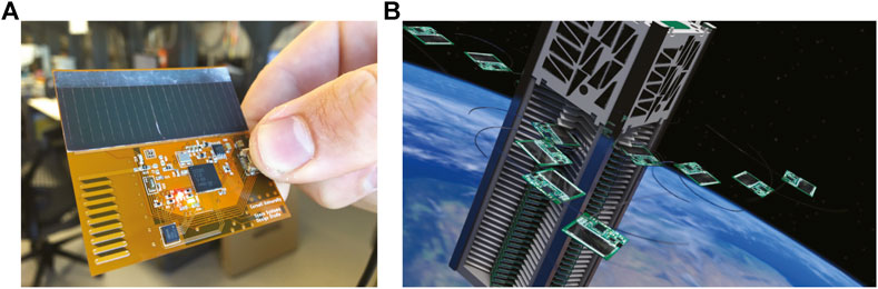
FIGURE 1. ChipSat and associated deployment concept. (A) Monarch ChipSat developed at Cornell University, (B) Artistic rendering of KickSat deployment phase [Image courtesy of Ben Bishop].

Through the methods described in this paper, we assess the Monarch’s suitability for planetary exploration missions in its current state and identify needed technology advancements.

3 Methods

3.1 Dynamics Model

3.1.1 Orbital Mechanics

The proposed model uses Cartesian coordinates in a planet-centered inertial frame. The position of a ChipSat, $\mathit{r}$, is therefore described by

$\mathit{r}=x\widehat{\mathit{i}}+y\widehat{\mathit{j}}+z\widehat{\mathit{k}}.(2)$

The equations of motion for the orbit are derived from a simplified geopotential model that ignores tesseral and sectorial effects. Only $J_2$ perturbation is considered (McClain and Vallado, 2001). The potential energy, $PE$, of the system is defined as

$PE=\frac{{\mu }_{\oplus }m}{\left|\left|\mathit{r}\right|\right|}+\frac{J_{2}m}{2||\mathit{r}{||}^5}\left(3z^2-||\mathit{r}{||}^2\right),(3)$

where ${\mu }_{\oplus }$ is the standard gravitational parameter

${\mu }_{\oplus }=-G{M}_{\oplus }.(4)$

The $J_2$ term in Eq. 3 is a function of the dimensionless $J_2$, labeled $J_{2,\dim }$ for distinction, according to

$J_2=J_{2,\dim }{\mu }_{\oplus }{R}_{\oplus }^2.(5)$

Introducing the Lagrangian,

$\mathrm{ℒ}=KE-PE.(6)$

and defining the kinetic energy, $KE$, as

$KE=\frac{1}{2}m{\dot{\mathit{r}}}^T\dot{\mathit{r}},(7)$

the equation of motion is solved for via the Euler-Lagrange equation.

$\frac{\partial \mathrm{ℒ}}{\partial r_i}-\frac{d}{dt}\frac{\partial \mathrm{ℒ}}{\partial {\dot{r}}_i}=0.(8)$

3.1.2 Aerodynamic Forces and Attitude Dynamics

While the dynamics of gram-scale spacecraft can become uniquely driven by the Lorentz force and solar pressure at higher altitude (Atchison and Peck, 2011), drag is the primary perturbing force in lower orbits. The drag force can be modeled according to

${\mathit{F}}_d=\frac{1}{2}Cd{\rho }_0{A}_{eff}{\Vert {\mathit{V}}_{sc}\Vert }^2\widehat{\mathit{v}},(9)$

where ${\rho }_0$ is the density of the surrounding atmosphere, and $A_{eff}$ is the area exposed to the instantaneous velocity vector $\widehat{\mathit{v}}$. Finally, ${\mathit{V}}_{sc}$ is the spacecraft’s velocity relative to the atmosphere, which is assumed to rotate with the planetary body at angular velocity ${\omega }_{\oplus }$

${\mathit{V}}_{sc}=\dot{\mathit{r}}-{\mathit{\omega }}_{\oplus }\times \mathit{r}.(10)$

The velocity vector $\widehat{\mathit{v}}$ is then defined as

$\widehat{\mathit{v}}=\frac{-{\mathit{V}}_{sc}}{\left|\left|{\mathit{V}}_{sc}\right|\right|}.(11)$

The drag coefficient and the effective area are both key parameters that determine the survivability of a planetary entry mission.

It is well understood that blunt bodies prove advantageous for atmospheric entry. At high velocities, a normal shock is detached from these geometries by an air cushion that forms ahead of the body. Such bow shocks dissipate 90 percent of the friction heat (Allen and Eggers, 1958). The theory explaining this was proposed by Julian Allen in the 1950s, and shaped the design of the Mercury capsule and many spacecraft thereafter.

A ChipSat oriented face-on to the incoming flow provides a more blunt shape than does an edge-on or tumbling ChipSat. Minimizing erothermal heating is a central goal for the proposed mission type. So, designing a ChipSat that can maintain this orientation is key. The effective area is therefore the cross-sectional area

$A_c=L^2,(12)$

where L is the side length of a square ChipSat. The face-on orientation also has a higher drag coefficient, which similarly works to the ChipSat’s advantage. Greater drag results in faster, and therefore earlier, deceleration. More of this deceleration occurs at higher altitudes where the atmosphere is less dense, thereby reducing the heat load.

In low Earth orbit, where the spacecraft is in the free molecular flow regime, the drag coefficient is modeled by (Storch, 2002)

$Cd=2\left[{\eta }_t+{\eta }_n\frac{V_w}{V_{sc}}\cos \alpha +\left(2-{\eta }_n-{\eta }_t\right){\cos }^2\left(\alpha \right)\right]\cos \left(\alpha \right).(13)$

Here, the angle of attack $\alpha$ is set to 90°. ${\eta }_n$ and ${\eta }_t$ are the molecular accommodation coefficients in the normal and tangential directions. Lastly, $V_w$ is the normal component of the average molecular velocity, defined as

$V_w=\sqrt{\frac{\pi R{T}_{sc}}{2M_{mol}}}(14)$

where R is the universal gas constant, $T_{sc}$ is the temperature of the spacecraft, and $M_{mol}$ is the molar mass of the surrounding atmosphere. Table 1 lists approximate values selected for these parameters in the model.

TABLE 1

TABLE 1. Simulation constants.

For sufficiently low ballistic coefficients, peak heating may occur while the spacecraft is still in the free molecular flow regime. A $1\text{cm}\times 1\text{cm}$ silicon wafer, the original concept for the ChipSats developed at Cornell, met this criterion (Atchison and Peck, 2011). For higher ballistic coefficients, corresponding to the PCB-based ChipSats developed in the past decade, peak heating occurs at lower altitudes. It is therefore important to account for the variation in drag coefficient across the free molecular, hypersonic, and subsonic regimes. A coefficient of 1.28 is attributed to a flat plate perpendicular to subsonic flow. (United States Air Force, 1965).

Supersonic and hypersonic drag coefficients, however, are very challenging to model. Experimental and computational work has shown that the drag coefficient depends on both flow parameters and wall temperature effects (Anderson, 2000). Due to the nature of the ChipSat’s low mass and ballistic coefficient, the decrease in $Cd$ from hypersonic to subsonic flow occurs over a very short time. For the model presented, the following bridging function pertains in the transition between free molecular and subsonic flow,

$Cd=\frac{C{d}_{SS}}{\sqrt{1+{\left(C{d}_{SS}/C{d}_{FM}\right)}^2}},(15)$

where $C{d}_{FM}$ and $C{d}_{SS}$ represent the free molecular and subsonic drag coefficients, respectively. Accounting for the shift toward lower drag coefficients also models the flight dynamics more accurately. As the ChipSat is at terminal velocity for tens of kilometers, the overall flight time depends heavily on the drag coefficients selected for the simulation.

Once the ChipSats are in the subsonic flow regime, their angle of attack is no longer critical to survival. Lift coefficients and force can therefore be considered as well. While maneuverable control surfaces on future generations of ChipSats is a possibility, this model describes spacecraft that remain oriented to the oncoming flow, through passive means. As a result, the ChipSats are modeled as drag-only throughout the entire duration of the descent, and equations of motion for ChipSat attitude are not explicitly included. It should be noted that this model also does not consider wind effects. While a wind model would certainly aid in the dispersion, this study seeks to generalize landing distribution predictions for cases where the wind patterns of the target planetary body may not be well understood. Swarm dispersion is therefore accomplished from drag alone, as a limiting case.

With the drag force established and separated into components, the complete translational equations of motion in Cartesian coordinates are

$\ddot{x}=-\frac{{\mu }_{\oplus }x}{\left|\left|{\mathit{r}}^3\right|\right|}+\frac{J_{2}x}{\left|\left|{\mathit{r}}^7\right|\right|}\left(6z^2-\frac{3}{2}\left(x^2+y^2\right)\right)+\frac{{\mathit{F}}_{d}x}{m\left|\left|\mathit{r}\right|\right|},(\mathrm{16a})$

$\ddot{y}=-\frac{{\mu }_{\oplus }y}{\left|\left|{\mathit{r}}^3\right|\right|}+\frac{J_{2}y}{\left|\left|{\mathit{r}}^7\right|\right|}\left(6z^2-\frac{3}{2}\left(x^2+y^2\right)\right)+\frac{{\mathit{F}}_{d}y}{m\left|\left|\mathit{r}\right|\right|},(\mathrm{16b})$

$\ddot{z}=-\frac{{\mu }_{\oplus }z}{\left|\left|{\mathit{r}}^3\right|\right|}+\frac{J_{2}z}{\left|\left|{\mathit{r}}^7\right|\right|}\left(3z^2-\frac{9}{2}\left(x^2+y^2\right)\right)+\frac{{\mathit{F}}_{d}z}{m\left|\left|\mathit{r}\right|\right|}.(\mathrm{16c})$

3.2 Thermal Model

The heating model employed for ChipSat deorbit and entry considers both convection and radiation. Heat radiated outward from a spacecraft at temperature $T_{sc}$ is calculated with respect to the planetary equilibrium temperature $T_{eq}$ according to

${\dot{Q}}_{\text{rad}}=-\sigma \epsilon A_s\left(T_{sc}^4-T_{eq}^4\right).(17)$

Here, σ is the Stefan-Boltzmann constant, and ε is the emissivity of the spacecraft material. A value of 0.85 reflects the Monarch design, which features a Kapton substrate. As heat can dissipate from both sides of the spacecraft, the surface area for this calculation is simply

$A_s=2A_c(18)$

It should be acknowledged that using $T_{eq}$ represents a worst-case hot condition. More realistically the surroundings may be colder at higher altitudes.

While in orbit, aerothermal heating is negligible. The spacecraft equilibrium temperature is determined from radiation and internal heat, ${\dot{Q}}_{\mathrm{int}}$, generated by the ChipSat. The Monarch features one $300\text{mW}$ solar cell on each face to ensure that the spacecraft can be powered in any orientation. For this model, it is assumed that $50\text{\%}$ of maximum power is converted to heat. As the focus of the thermal model is calculation of maximum temperature during entry, temperature fluctuations due to eclipse portions of the orbit are not considered.

Drag eventually drives the spacecraft’s orbit down to the upper atmosphere, where convection comes into play. Aerodynamic heating is modeled by

${\dot{Q}}_{\text{aero}}=\frac{1}{2}ST{\rho }_0{A}_{eff}{\Vert {\mathit{V}}_{sc}\Vert }^3,(19)$

where ${\rho }_0$ is the density of the surrounding atmosphere and $A_{eff}$ is once again the cross sectional area. The coefficient $ST$ is the Stanton number, a dimensionless value that represents the ratio between the actual heat flux to the fluid and the maximum possible enthalpy change (Lienhard, 2019). It corresponds to skin friction and is a function of the flow regime. For free molecular flow, the Stanton number maintains a constant value of 1 that is independent of the body shape Koppenwallner et al. (2001). For continuum flow, the Stanton number is a function of the Reynolds number after the shock, ${\mathit{Re}}_2$ and shape parameter $C_S$. For rarefied transitional flow, a bridging function is used. This variation is summarized as follows (Koppenwallner et al., 2001):

$Kn>10$ Free molecular flow

$S{T}_{FM}=1.(\mathrm{20a})$

$10>Kn>0.01$ Rarefied transitional flow

$ST=\frac{S{T}_C}{\sqrt{1+{\left(S{T}_c/S{T}_{FM}\right)}^2}}.(\mathrm{20b})$

$0.01>Kn$ Hypersonic continuum flow

$S{T}_C=\frac{2.1C_s}{\sqrt{{\mathit{Re}}_2}},(\mathrm{20c})$

where the flow regimes are determined by the Knudsen number $Kn$. The Knudsen number is a dimensionless flow parameter defined as the ratio of the mean free path λ to characteristic length L, the length of the ChipSat. The mean free path is the average distance traveled by a molecule between successive impacts (Chapman et al., 1990). It is a function of the dynamic viscosity ${\mu }_0$, temperature $T_0$, density, and molar mass of the surrounding gas.

$\lambda =\frac{{\mu }_0}{{\rho }_0}\sqrt{\frac{\pi M_{\text{mol}}}{2N_A{k}_b{T}_0}},(21)$

where $N_A$ and $k_b$ are Avogadro’s number and the Boltzmann number, respectively. The Knudsen number can be calculated based on this expression, or as a function of the local Mach and Reynolds numbers.

$K{n}_0=\frac{\lambda }{L}=\sqrt{\frac{\pi \gamma }{2}}\left(\frac{Ma}{\mathit{Re}}\right),(22)$

$\mathit{Re}=\frac{{\rho }_0\Vert {\mathit{V}}_{sc}\Vert L}{{\mu }_0},(23)$

$Ma=\frac{\Vert {\mathit{V}}_{sc}\Vert }{{\mathit{V}}_{\text{sound}}}=\sqrt{\frac{M_{\text{mol}}{\Vert {\mathit{V}}_{sc}\Vert }^2}{\gamma R{T}_0},}(24)$

where γ is the isentropic expansion factor, and $V_{\text{sound}}$ is the local speed of sound. In either case, models for how temperature, density, dynamic viscosity and molar mass vary with altitude are necessary to determine the flow regime. Assuming an ideal gas, molar mass can be obtained from temperature, density, and pressure $P_0$ according to

$M_{\text{mol}}=\frac{{\rho }_{0}R{T}_0}{P_0}.(25)$

Additionally, dynamic viscosity can be expressed as a function of temperature according to Sutherland’s law (White, 2006)

$\frac{{\mu }_0}{{\mu }_r}={\left(\frac{T_0}{T_r}\right)}^{\frac{3}{2}}\frac{T_r+S_{\mu }}{T_0+S_{\mu }},(26)$

where ${\mu }_r$ and $T_r$ are the reference viscosity and temperature, and $S_{\mu }$ is the Sutherland temperature. All three values are specific to the gas and are listed in Table 2. With these relations established, the flow regime, and subsequently the Stanton number, can be determined solely from altitude-based models of temperature, pressure, and density. The relationship between Stanton, Knudsen, and Reynolds number is shown for a sample Earth entry simulation in Figure 2. For the purposes of this study, spatially and temporally varying atmospheric models are not considered. The atmospheric data used in these calculations only varies with altitude. Similar to the selection of a wind-free model, this decision was made for both ease of computation during batch simulations, as well as to generalize the predictions for planetary bodies where temperature, pressure, and density models are not yet so refined.

TABLE 2

TABLE 2. Planetary entry simulation parameters and results.

FIGURE 2

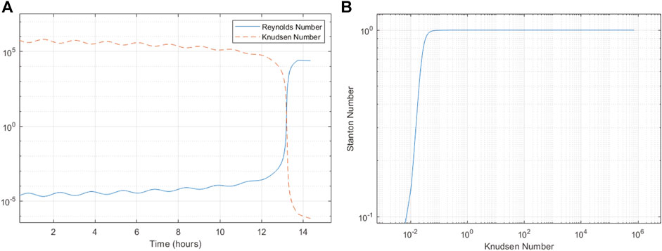
FIGURE 2. Relation between flow characterization parameters, (A) time-histories of Reynolds number and Knudsen number for Monarch ChipSat Earth entry, (B) Stanton number vs. Knudsen number.

Returning to Eq. 20c, isentropic flow is assumed. This assumption permits the use of algebraic expressions that relate properties behind the shock to the gas stagnation conditions upstream of the shock (Forney et al., 1987). The local Reynolds number ${\mathit{Re}}_2$ is defined as

${\mathit{Re}}_2={\left(\frac{\pi \gamma }{2}\right)}^{\frac{1}{2}}\left(\frac{1}{K{n}_2}\right)M_{{\mathit{p}}_2},(27)$

where $K{n}_2$ and $M_{p_2}$ are respectively the Knudsen number and particle Mach number immediately behind the shock. These parameters are related to upstream conditions according to (Forney et al., 1987)

$K{n}_2=K{n}_0\left(\frac{{\rho }_1}{{\rho }_2}\right)\left(\frac{{\rho }_0}{{\rho }_1}\right),(28)$

$M_{p_2}=\frac{{\left(2/\left(\gamma -1\right)\right)}^{\frac{1}{2}}\left(M{a}^2-1\right)}{{\left[1+\left(\left(\gamma -1\right)/2\right)M{a}^2\right]}^{\frac{1}{2}}{\left[\left(2\gamma /\left(\gamma -1\right)\right)M{a}^2-1\right]}^{\frac{1}{2}}}.(29)$

where ${\rho }_1$ and ${\rho }_2$ are respectively the gas densities immediately in front of and behind the shock as shown in Figure 3. The density ratios of Eq. 28 are expressed as functions of the Mach number and the specific heat ratio.

$\frac{{\rho }_0}{{\rho }_1}={\left[1+\left(\frac{\gamma -1}{2}\right)M{a}^2\right]}^{\frac{1}{\gamma -1}},(30)$

$\frac{{\rho }_1}{{\rho }_2}=\frac{\left(\gamma -1\right)M{a}^2+2}{\left(\gamma +1\right)M{a}^2}.(31)$

FIGURE 3

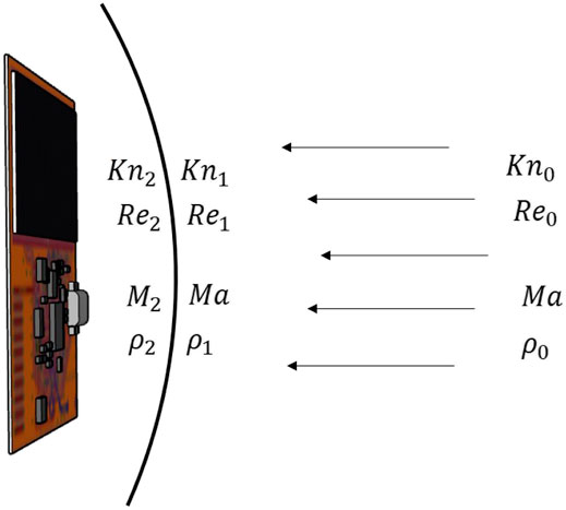
FIGURE 3. Flow parameters for a detached bow shock, (0) gas stagnation conditions upstream of the shock, (1) gas properties near the shock front, (2) gas properties immediately after the shock. Mach number remains constant ahead of the shock [ChipSat CAD model courtesy of Andrew Filo].

With the Stanton number established for hypersonic continuum flow, it is now possible to model aerodynamic heating across all flow regimes in order to predict peak reentry temperatures. The following first order differential equation is used to solve for ChipSat temperature $T_{sc}$ as a function of convection, radiation, and internally generated heat

${\dot{T}}_{sc}=\frac{{\dot{Q}}_{\mathrm{int}}+{\dot{Q}}_{\text{aero}}+{\dot{Q}}_{\text{rad}}}{m{c}_p},(32)$

where $c_p$ is the specific heat of the spacecraft material. See Table 1 for the value selected for the Monarch. Eqs 16, 32 are the four differential equations needed to model the dynamics of the ChipSat’s deorbit and planetary entry.

4 Case Studies

With the proposed aerothermal model, four simulations were carried out to assess the landing distribution and potential for survival of the Monarch ChipSat. The planetary bodies selected are Earth, Mars as a representation of planets with thinner atmospheres, Titan to represent celestial bodies with thicker atmospheres, and lastly the Moon as a reference point that reflects bodies with no atmosphere. In each case, the initial conditions assume deployment from an orbiter. This deployer could be a CubeSat, such as those used in the KickSat missions, that stores the ChipSats in a stacked configuration to radially eject. Figure 1B illustrates this concept.

100 Monarch ChipSats are deployed in a Monte Carlo simulation for each case study. Their initial position is randomized by a Gaussian distribution to reflect their placement within their stack in a 3U CubeSat. The initial velocity of each ChipSat includes an ejection velocity of $1\text{m}/\text{s}$. Each ChipSat is attributed a unique deployment direction to establish a $360°$ spread of the swarm. While approximate, these conditions are reflective of past missions. A similar variation in deployment height and direction can be found from a spin-stabilized deployer that successively ejects rows of stacked ChipSats through a spring-loaded release mechanism (Manchester et al., 2013). This kick is added to the orbital velocity, $V_{\text{orb}}$, of the deployer.

$V_{\text{orb}}=\sqrt{\frac{G{M}_{\oplus }}{R_{\oplus }+h_o}}.(33)$

Equation 33 is simply the expression for the velocity of a circular orbit and is determined by the deployment altitude $h_o$. $M_{\oplus }$ and $R_{\oplus }$ are the mass and radius of the planetary body, respectively, and G is the gravitational constant. Lastly, randomization is once again introduced to account for small variations in ChipSat mass and area which may arise during conformal coating. Each ChipSat is randomly assigned a mass according to a Gaussian distribution with a mean of 3 g (the mass of a conformal coated Monarch) and a standard deviation of 0.1 g. Each is similarly ascribed an area with a mean of $25{\text{cm}}^2$ and $1\text{\%}$ standard deviation. See Tables 1, 2 for a full list of parameters and initial conditions.

4.1 Earth

The simulation commences in low Earth orbit, with an initial altitude of $350\text{km}$ and a 50° inclination. This is approximately the orbit of a CubeSat deployed from the ISS that has gradually lost altitude to drag. Temperature, pressure, and density values throughout the descent are taken from the U.S. Standard Atmosphere, 1976 (NOAA, 1976). Polynomial fits are employed for the majority of the data. For altitudes below $86\text{km}$, the geopotential altitude, $h_{gp}$ is calculated for compatibility with more precise MATLAB functions.

$h_{gp}=\frac{R_{\oplus }}{\Vert \mathit{r}\Vert }h.(34)$

The temperature and density model is shown in Figure 4.

FIGURE 4

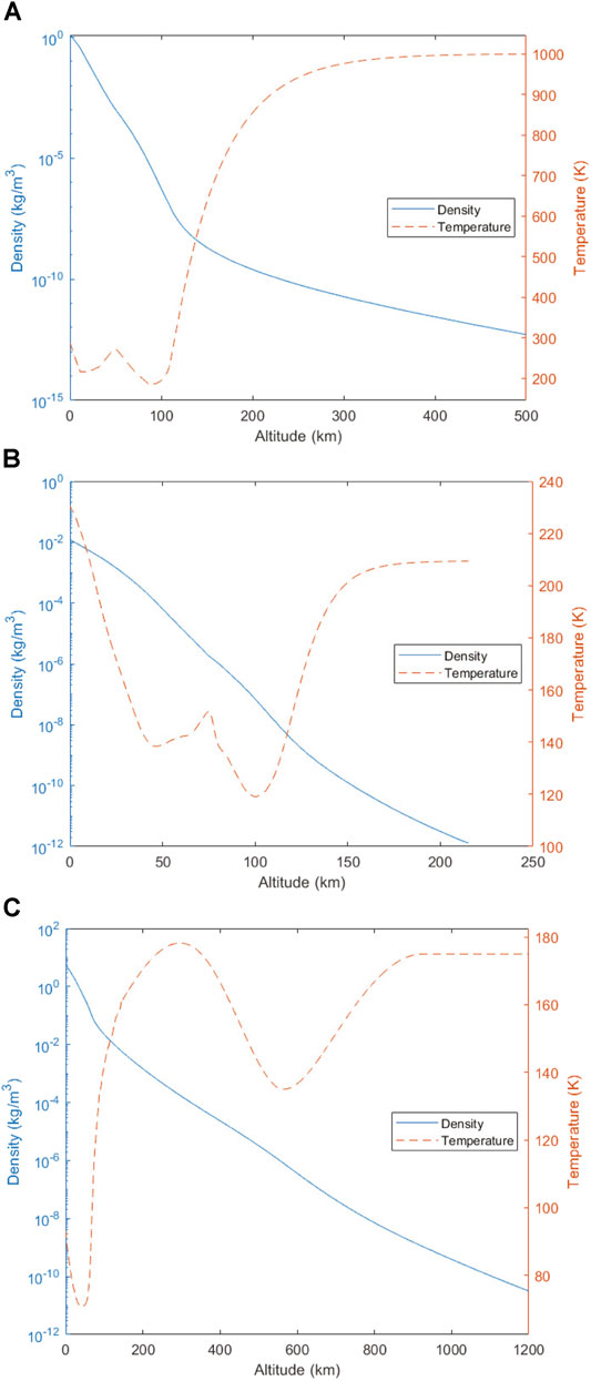
FIGURE 4. Density and temperature models for ChipSat atmospheric entry simulations, (A) Earth (US Standard Atmosphere, 1976), (B) Mars (Mars-GRAM 2010), (C) Titan (Yelle Model).

Figure 5A displays the descent from orbit and the temperature spike for a single ChipSat. In this simulation, the mean values are used for area and mass, and no height randomization or deployment kick is given. In orbit, the Monarch settles on an equilibrium temperature of −8.8°C and reaches a peak temperature of 840°C upon entry at an altitude of $89.3\text{km}$. The temperature results suggest that the Monarch ChipSat cannot survive Earth entry in its current form. The peak temperature is within range of the melting points of high-temperature solder, and is far above the operating and storage temperatures of most of the electronics on board. While FR-4 substrates would melt during atmospheric entry, the Kapton substrate of the Monarch is likely to retain its integrity. Due to the very short duration of the high temperatures, it is possible that with some modifications such a ChipSat could remain intact for operation on the ground. Possible design solutions are discussed in Section 5.3.

FIGURE 5

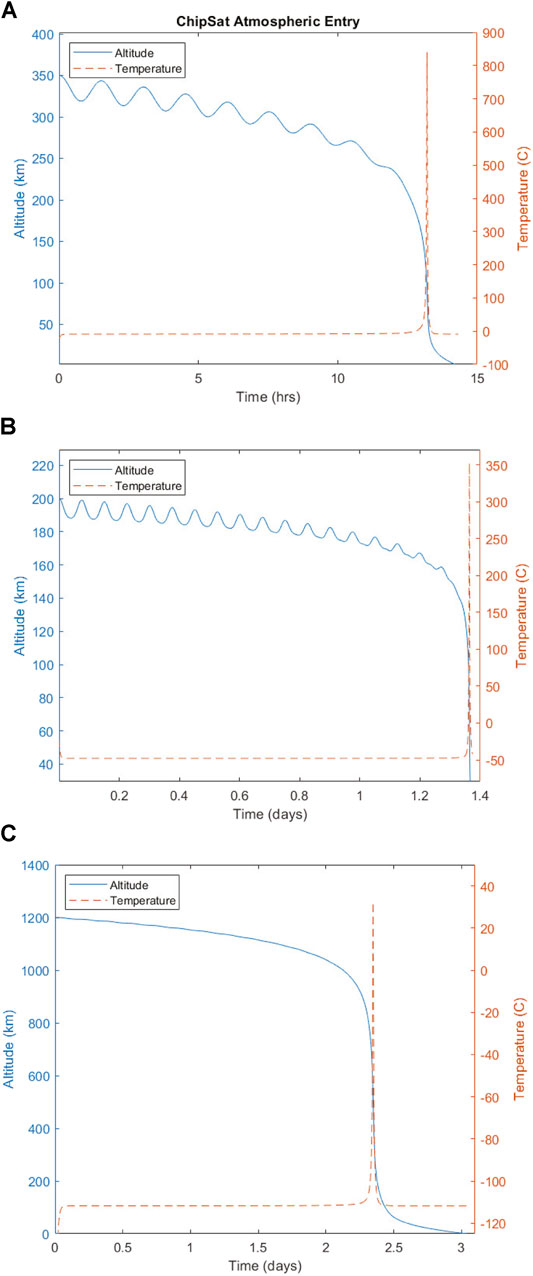
FIGURE 5. Altitude and temperature time-histories of face-on atmospheric entry of Monarch ChipSat, (A) Earth, (B) Mars, (C) Titan.

Figure 6A provides a close up of the temperature spike with the local Mach number overlaid. The maximum value of Mach 22 occurs approximately 1 minute before the peak temperature. The subsequent and rapid drop of both values coincide as the ChipSat reaches terminal velocity within minutes. Figure 7A conveys the change in flight-path angle ϕ during this deceleration. Within 3 minutes of reaching a peak drag of $84.3{\text{km/s}}^2$, the ChipSat dissipates all of its excess kinetic energy and descends in free fall $\left(\varphi =90\right)$. The ChipSat then falls at terminal velocity for just over 1 hour before impacting the ground at a speed of $3.87\text{m/s}$. The same value can also be obtained by the following expression.

$V_{\text{term}}=\sqrt{\frac{2{\mu }_{\oplus }m}{\rho \left(h\right)A_{c}Cd{\left(R_{\oplus }+h\right)}^2}}=\sqrt{\frac{2\beta {\mu }_{\oplus }}{\rho \left(h\right){\left(R_{\oplus }+h\right)}^2}},(35)$

where density is a function of altitude, h, which is set to zero for the landing case, and the subsonic value of 1.28 is attributed to $Cd$. The entire descent from $350\text{km}$ takes approximately 14 h and 20 min.

FIGURE 6

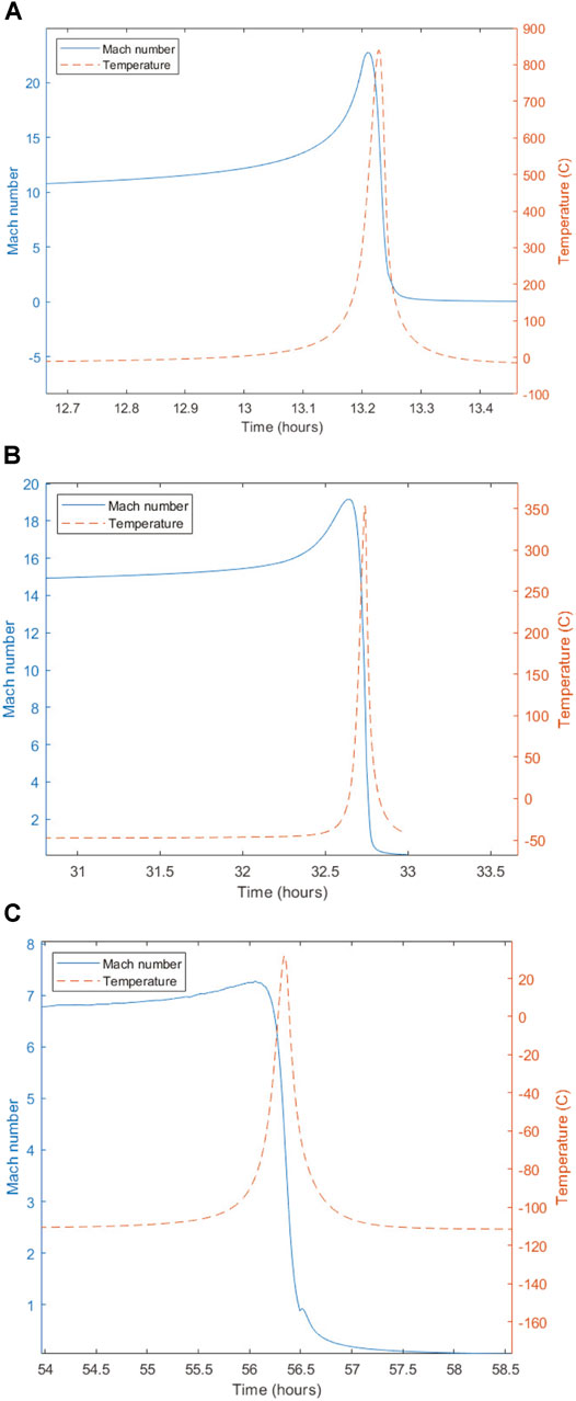
FIGURE 6. Mach number and temperature time-histories of face-on atmospheric entry of Monarch ChipSat, (A) Earth, (B) Mars, (C) Titan.

FIGURE 7

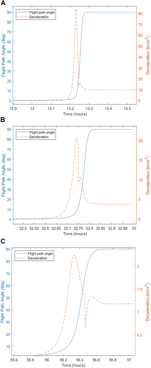
FIGURE 7. Flight path angle, ϕ, and drag deceleration time-histories of face-on atmospheric entry of Monarch ChipSat, (A) Earth, (B) Mars, (C) Titan.

The results of the Monte Carlo simulation are shown in Figures 8A, 9A. The radial deployment and small perturbations in ChipSat mass and area are sufficient to achieve staggered deorbit times, resulting in a global distribution. As this model does not consider wind effects, the landing locations of the ChipSats are aligned according to the inclination of the original orbit. The small deviances are solely from the initial deployment direction. Global wind models, although computationally expensive, would augment the scattering from the ground track of the deployer spacecraft if implemented.

FIGURE 8

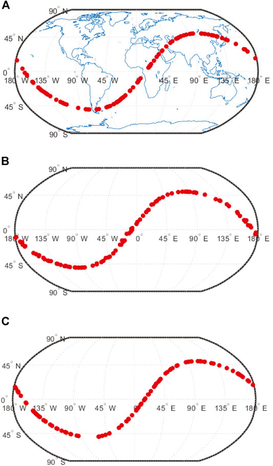
FIGURE 8. Landing locations for Monte Carlo simulation of Monarch ChipSat atmospheric entry, 50 $°$ inclination. (A) Earth, (B) Mars, (C) Titan.

FIGURE 9

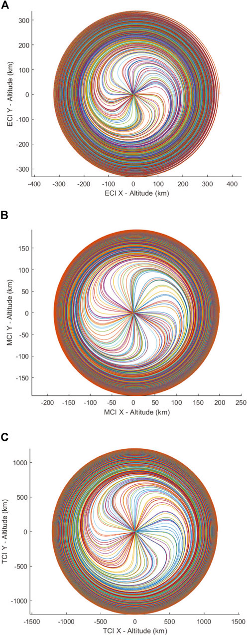
FIGURE 9. Deorbit trajectories for Monte Carlo simulation of Monarch ChipSat atmospheric entry, equatorial orbit. (A) Earth, (B) Mars, (C) Titan.

4.2 Mars

Due to the thinner atmosphere, deorbit simulations on Mars are initiated at a $200\text{km}$ circular orbit. The same 50$°$ inclination is selected for a more direct comparison to the Earth case. The Mars-GRAM 2010 dataset is used to obtain temperature, pressure, and density values throughout the descent (Justh et al., 2011). The temperature and density model based on interpolated table data is shown in Figure 4B.

Figure 5B displays the descent from orbit and the temperature spike for a single ChipSat with no randomization of parameters. In orbit, the Monarch settles on an equilibrium temperature of −47.8°C and reaches a peak temperature of 353°C upon entry at an altitude of $66\text{km}$. The temperature results suggest that the Monarch ChipSat stands a better chance in a Mars entry, but it would still have difficulty operating in its current state. The peak temperature is sufficiently below both the melting point of high-temperature solder and the max temperature rating of the Kapton substrate. However, it is still far above the operating and storage temperatures of most of the electronics on board. Given the short duration of the high-temperature exposure, it is possible that the electronics would remain operational for the remainder of the descent. The equilibrium temperature is just below the lower range of the Monarch’s components, suggesting that continuous operation in orbit and on the Martian surface is possible (provided there is sunlight). Experimental validation would help resolve this uncertainty.

Figure 6B shows that the maximum value of Mach 19 occurs approximately 6 minutes before the peak temperature, which occurs at the same time as the peak drag of $20.7{\text{km/s}}^2$. From Figure 7B it is shown that within 5 minutes of peak drag, the ChipSat is in free fall $\left(\varphi =90\right)$ after dissipating all of its excess kinetic energy. Due to the thin atmosphere, the ChipSat descends at terminal velocity for only 12 minutes before impacting the ground at a speed of $24\text{.}05\text{m}/\text{s}$. This result is consistent with Eq. 35. The entire descent from $200\text{km}$ takes approximately 1 day and 9 h.

The results of the Monte Carlo simulation are shown in Figures 8B, 9B. The radial deployment and small perturbations in ChipSat mass and area are again sufficient to achieve staggered deorbit times, resulting in a global distribution. As this model does not consider wind effects, the landing locations of the ChipSats are also only slightly deviated from the ground track of the original orbit.

4.3 Titan

With its dense atmosphere, maintaining orbit around Titan requires significantly higher altitudes. Deorbit simulations are initiated at a $1200\text{km}$ circular orbit. The same 50$°$ inclination is selected for a more direct comparison to the prior two cases. The Yelle model provides temperature, pressure, and density values throughout the descent (Yelle et al., 1997). The temperature and density model based on interpolated table data is shown in Figure 4C.

Figure 5C displays the descent from orbit and the temperature spike for a single ChipSat with no randomization of parameters. In orbit, the Monarch settles on an equilibrium temperature of −111.7°C and reaches a peak temperature of 32.1°C upon entry at an altitude of $512\text{km}$. The temperature results indicate that using ChipSats for distributed atmospheric sensing on Titan is feasible with high certainty. The peak temperature is far below the melting point of commercial-grade solder and is well within the temperature rating of both the Kapton substrate and the electronic components on board. Due to Titan’s distance from the sun, however, the Monarchs would need key modifications. Solar power would no longer be sufficient, and the equilibrium temperature before and after entry is far below the operating and storage temperatures of the circuit components. Small-scale betavoltaic power sources, such as those used in pacemakers, may provide an alternative power source for a Titan ChipSat mission. Combined with additional insulation, betavoltaics may provide sufficient heat for continuous sensing in orbit and on Titan’s surface.

Figure 6C provides a close up of the temperature spike with the local Mach number overlaid. The maximum value of Mach 7 occurs approximately 17 minutes before the peak temperature, which corresponds to the peak in deceleration due to drag. From Figure 7C it is shown that within 19 minutes of peak drag of $2\text{.}26\text{km}/{\text{s}}^2$, the ChipSat is in free fall $\left(\varphi =90\right)$ after dissipating all of its excess kinetic energy. The ChipSat then descends at terminal velocity for 17 hours before impacting the ground at a speed of $\text{0}\text{.}68\text{m}/\text{s}$. This result is consistent with Eq. 35. The entire descent from $1200\text{km}$ takes just under 3 days and 1 h, enabling recording of a large dataset.

The results of the Monte Carlo simulation are shown in Figures 8C, 9C. The radial deployment and small perturbations in ChipSat mass and area are once again sufficient to achieve staggered deorbit times, resulting in a global distribution. As this model also does not consider wind effects, the landing locations of the ChipSats only slightly deviate from the ground track of the original orbit. Given the extended descent at terminal velocity, which begins at $\text{∼}500\text{km}$, wind would have a significant impact on the final landing distribution on Titan.

4.4 Moon

For comparison, we examine the case of no atmosphere with a ChipSat deployment on the Moon. Without drag, sufficient deceleration for deorbit must be imparted during deployment. All dispersion of the swarm also comes from varied initial conditions during ejection from the deployer. In this scenario, a mothership in a $100\text{km}$ circular orbit ejects a deployer, which in turn releases 100 ChipSats into a landing trajectory. For simplicity, an equatorial orbit is selected, and oblateness is not considered. The initial velocity for a landing trajectory, $V_{\text{land}}$ can be found from the vis-viva equation (McClain and Vallado, 2001)

$V_{\text{land}}={\mu }_{\oplus }\sqrt{\frac{2}{\left|\left|\mathit{r}\right|\right|}-\frac{1}{a}}={\mu }_{\oplus }\sqrt{\frac{2}{R_{\oplus }}-\frac{2}{2R_{\oplus }+h_o}},(36)$

where a is the orbit semi-major axis. The landing trajectory is an elliptical orbit with apoapsis at the $100\text{km}$ initial altitude and periapsis at the lunar surface. Inputting these parameters, Eq. 36 provides a desired initial velocity of $1611m/s$. As the mothership in this scenario is traveling at a higher velocity in circular orbit according to Eq. 33, the minimum $\Delta V$ required to land the ChipSats is simply −23 m/s according to

$\Delta V=V_{\text{orb}}-V_{\text{land}}.(37)$

This change in velocity may be achieved from a cold-gas thruster or a spring-loaded mechanism that pushes the deployer in retrograde from the mothership. Once separated and traveling at the desired velocity, the deployer then radially ejects the ChipSats at $5\text{m}/\text{s}$ for dispersion and landing. To accommodate for the additional velocity of ChipSats dispersion (some of which may be prograde), $-5\text{m}/\text{s}$ is added to the $\Delta V$ of the deployer separation as well, for a total $\Delta V$ of $-28\text{m}/\text{s}$.

The results of the lunar deployment are shown in Figure 10. Fluctuations in solar exposure are once again neglected, resulting in a constant spacecraft equilibrium temperature of $5.5°C$ throughout that is well within the operating conditions of the Monarch. The swarm of 3-gram ChipSats spans several kilometers. The landing ellipse has a semi-major axis of $156\text{km}$ and a semi-minor axis of $4\text{.}2\text{km}$. The high eccentricity of the ellipse is caused by certain ChipSats ejecting nearly directly prograde or retrograde to the deployer trajectory. Those deployed with a greater lateral velocity component do not deviate as much from the original flight path. The flight times for each Monarch range from 39 min and 40 s to 42 min and 40 s. At this point, they impact the lunar surface with a velocity of $1703\text{.}6\text{m}/\text{s}$.

FIGURE 10

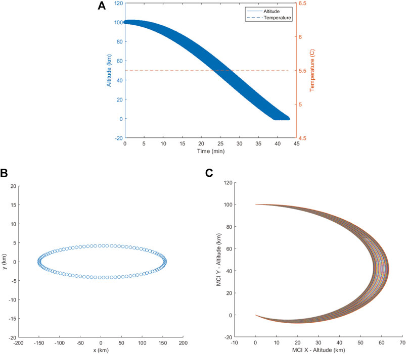
FIGURE 10. Monarch ChipSat lunar landing case study, (A) altitude and temperature time-history, (B) landing ellipse, (C) swarm trajectories.

This landing velocity is significantly higher than the terminal velocities encountered for planetary bodies with atmospheres. The greatest risk to the ChipSat’s survival during such a mission becomes its impact with the surface, followed by radiation. Both of these factors have been investigated by research at Cornell. In 2017, Hunter Adams conducted a durability study in which 12 FR-4 based ChipSats were exposed to accelerations ranging from 5,000 to 27,0000 g’s via an elastically loaded drop table (Adams and Peck, 2019). The ChipSats were placed on lunar regolith simulant to resemble impact with the Moon’s surface. Sensor readings from the most sensitive component on board, the IMU, were used as metric for survival. Measurements were taken after each impact, and each sensor continued to perform within manufacturer specifications. Here, the ChipSat’s scale once again proves advantageous. Smaller objects exhibit higher natural structural frequencies and approach continuous materials like crystals, making them less susceptible to high strain and crack propagation and therefore more capable of withstanding shock.

Regarding long-term survival of these minimalist COTS-based spacecraft, an experiment was conducted in 2011 in which three early-prototype ChipSats were brought to the ISS on board STS-134 (Manchester and Peck, 2011). They were mounted outside the space station as part of the MISSE-8 experimental pallet, where they were exposed to extreme temperatures, vacuum, and radiation for a period of three years. When retrieved in 2014, two of the three ChipSats were fully operational and the third showed partial functionality. While both of these experiments offer some insight into the survival statistics, no specific ChipSat can be guaranteed to survive. Nevertheless, these experiments do suggest a non-zero probability of success for a swarm of ChipSats. Mission assurance for ChipSats is statistical in nature. Like many R-selected species, survival is based on numbers. This is a stark contrast to the high-cost-for-low-risk approach for traditional spacecraft. The experiments conducted thus far therefore present strong evidence that a portion of deployed ChipSats would survive impact with celestial bodies and subsequently operate for the long term in the space environment.

5 Parametric Study

5.1 Role of the Ballistic Coefficient

Returning to the set up of the batch simulations, the four randomized factors are deployment direction, height within the deployer, mass, and area. Figures 11A,B present histograms for peak temperature and deorbit time in the Earth entry simulation. Both histograms resemble Gaussian distributions, reflecting the randomization used on the initial conditions. Peak entry temperatures have a mean value of 841°C with a standard deviation of 8.653°C. Deorbit times have a mean of 14.4 h with a standard deviation of 23.4 min. In an effort to correlate the distribution of temperatures and deorbit times to the variation in initial conditions, we revisit the ballistic coefficient.

FIGURE 11

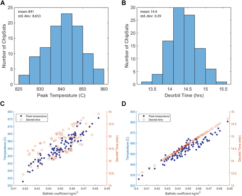
FIGURE 11. Correlation between peak temperature/deorbit time and ballistic coefficient, β, for Monarch ChipSat Earth entry Monte Carlo simulation, (A) Histogram of peak temperatures, (B) Histogram of deorbit times, (C) peak temperature and deorbit time vs. β for randomized deployment conditions, (D) peak temperature and deorbit time vs. β for identical initial deployment.

Figure 11C plots both variables with respect to the ballistic coefficient, β, presenting a strong positive correlation. To hone in on the dependence on β, the 100 ChipSat simulation is run again, but this time with identical deployment height, and no radial kick. With small variations only in mass and area, there is a much cleaner positive correlation shown in Figure 11D. This is especially true for deorbit time, which now appears almost perfectly linear.

5.2 Parametric Search

These correlations emerging for small perturbations in the Monarch’s ballistic coefficient motivate widening the scope. A parametric study is conducted for the Earth entry case. 400 simulations are run in which ChipSat mass is incremented from 1 mg to 8 g, and side length is incremented from $5\text{mm}$ up to $10\text{cm}$. The correlations on this larger scale are shown in Figures 12A,B. For the lowest ballistic coefficients $\left(\beta <<1\text{kg}/{\text{m}}^2\right)$, the ChipSat can enter Earth’s atmosphere without even breaking a sweat. Such ballistic coefficients cannot be achieved from PCB-based ChipSats, but perhaps from a thinner silicon-wafer variant (Atchison et al., 2010). As a reference, a conformal coated Monarch has a β of $0.45\text{kg}/{\text{m}}^2$. For the largest ballistic coefficient $\left(\beta =120\text{kg}/{\text{m}}^2\right)$ corresponding to the iteration with the largest mass and smallest area, peak temperatures soar to 5000°C. This temperature is just below the peak encountered by steep-trajectory, medium-range ballistic missiles decades prior to the development of Allen’s Blunt Body Theory (Launius et al., 2012).

FIGURE 12

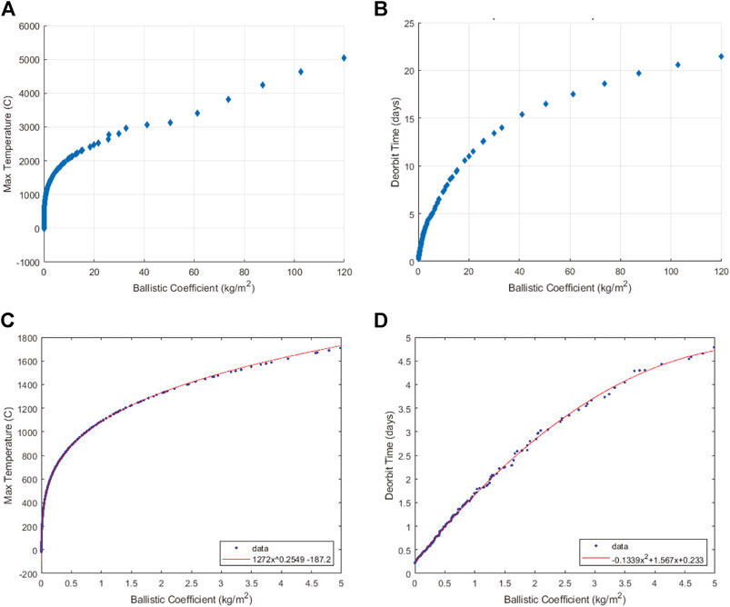
FIGURE 12. Correlation between peak temperature/deorbit time and ballistic coefficient, β, for parametric study of ChipSat Earth entry, (A) peak temperature vs. β, (B) deorbit time vs. β, (C) peak temperature curve fitting for low β, (D) deorbit time curve fitting for low β

For both peak temperature and time to ground, there is a strong, although non-linear, correlation with ballistic coefficient. This relation is more clearly defined for lower β values, a subset that contains all ChipSats developed thus far. Figures 12C,D provide a closer look at ballistic coefficients below $5\text{kg}/{\text{m}}^2$. For low ballistic coefficients, the relation to peak temperature and deorbit time is so well defined that a power fit and quadratic fit can be used, respectively. Thus, provided with only the ballistic coefficient these two functions can be used to assess ChipSat survival and mission duration.

5.3 Future ChipSat Design

Figure 13 provides an alternative visualization for peak temperatures to assist with design decisions. The Monarch with its peak temperature of 840°C is indicated by a red dot for reference. If planning a ChipSat mission for in-situ atmospheric sensing, ChipSat designers must be conscious of the need to maximize the surface area to mass ratio. Simply assembling the Monarch on a Kapton board that is double the side length would drop peak temperatures by 300°. While decelerating higher in the atmosphere improves chances for survival, it also shortens the time in orbit. Quadrupling the area in this case would result in a 32$\text{\%}$ decrease in mission duration. One solution to optimize both flight time and survivability is a shape-shifting ChipSat. Through a lightweight nitinol-wire frame, a $10\text{cm}$ Monarch could be folded down into $5\text{cm}\times 5\text{cm}$ for the majority of the mission in the upper atmosphere. Closer to when peak drag occurs, driving current through the nitinol expands the ChipSat to $10\text{cm}\times 10\text{cm}$. Effectively, the ChipSat becomes its own parachute. In addition to more drag, the unfolding increases the surface area available for radiative cooling. The expansion would be autonomous, and could simply be triggered by a threshold temperature or pressure.

FIGURE 13

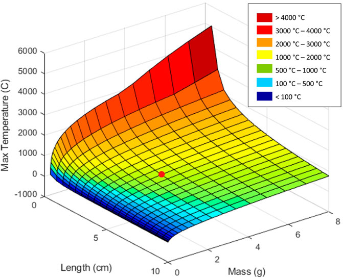
FIGURE 13. Parametric analysis of ChipSat Earth entry, with Monarch indicated by red dot for reference.

A mission ConOps such as this would take advantage of the larger area when it is needed most. However, adjusting the ballistic coefficient alone may not be enough. As a start, swapping the on-board electronics for military-grade IC’s would increase the maximum operating temperature from $85°\text{C}$ to $125\text{°C}$. While this is certainly an improvement, additional cooling mechanisms are still needed. Perhaps several current-activated cooling fins could pop up behind the ChipSat during the descent. Such a design would require a more intricate nitinol frame, but it may prove very effective if implemented in such a way that the additional mass is minimal. As the electronics on board compose a large portion of the ChipSat’s mass, they will likely remain oriented to the oncoming flow. One consideration should be to move the most sensitive components toward a back side or heat fin, again a complicated design. More simply or perhaps concurrently, additional shielding may be applied to the frontal flow-facing surface. The shielding could be a lightweight ablative coating, or perhaps a ceramic thermal barrier coating (TBC) used in gas turbine blades. For most PCB-based ChipSats $\left(0.1<\beta <1.5\text{kg}/{\text{m}}^2\right)$, some form of shielding is essential for the final stretch to achieve safe operating temperatures throughout the descent.

6 Conclusion

ChipSats enable a new kind of exploration. Planetary entry missions for distributed in-situ sensing—both on the ground and in the atmosphere—can now be designed with a low-cost-high-risk approach. The model presented demonstrates that while a swarm of Monarchs may have difficulty surviving entry back to Earth, they stand a better chance in both the thinner atmosphere of Mars, and the thicker atmosphere of Titan. Given the advantages of their scale and the lack of thermal concerns in the no-atmosphere case, the Monarchs may even fare well during a high-velocity impact on the Moon. With an understanding of the methods developed, one can engineer the ChipSat to meet the requirements of the environmental extremes. A lower ballistic coefficient, combined with additional surfaces for radiative cooling and protective coatings for flow-facing components, may be sufficient for survival in the more challenging entry cases. Additional work can be done to characterize the terminal-velocity phase of the descent—flat plates tend to exhibit intricate motions in free fall that may increase dispersion range—but the current model demonstrates that a global distribution of ChipSats is possible from drag alone. Such missions could produce datasets of spatially-varying phenomena throughout the solar system in unprecedented detail.

Data Availability Statement

The datasets presented in this study can be found in online repositories. The names of the repository/repositories and accession number(s) can be found below: https://github.com/JUmanskyCastro/ChipSats-for-Planetary-Exploration.

Author Contributions

JU led the conception and design of the study, and wrote the first draft of the manuscript. KY prepared atmospheric models, assisted with code development, and prepared the majority of the figures. MP advised the design of the study, reviewed the first draft of the manuscript, and contributed to the final version.

Funding

This work was made possible thanks to funding from the GEM Fellowship Program, the Alfred P. Sloan Foundation, and the Cornell Colman Fellowship.

Conflict of Interest

The authors declare that the research was conducted in the absence of any commercial or financial relationships that could be construed as a potential conflict of interest.

Acknowledgments

Thank you to Hunter Adams for his guidance with the orbital dynamics and code-debugging during our early simulation attempts, as well as the enjoyable conversations imagining futuristic concepts for next-generation ChipSats. The authors would also like to express thanks to Ralph Lorenz at APL for providing the Titan atmospheric data used in this study.

References

Allen, H., and Eggers, A. (1958). A Study of the Motion and Aerodynamic Heating of Ballistic Missiles Entering the Earth’s Atmosphere at High Supersonic Speeds. Tech. Rep. 1381, NASA Ames.

Google Scholar

Anderson, J. (2000). Hypersonic and High Temperature Gas Dynamics. McGraw-Hill series in aeronautical and aerospace engineering (American Institute of Aeronautics and Astronautics).

Atchison, J. A., Manchester, Z., and Peck, M. (2010). Microscale Atmospheric Re-entry Sensors (International Planetary Probe Workshop).

Atchison, J. A., and Peck, M. A. (2011). Length Scaling in Spacecraft Dynamics. J. guidance, Control Dyn. 34, 231–246. doi:10.2514/1.49383

CrossRef Full Text | Google Scholar

Chapman, S., Cowling, T., Burnett, D., and Cercignani, C. (1990). The Mathematical Theory of Non-uniform Gases: An Account of the Kinetic Theory of Viscosity, Thermal Conduction and Diffusion in Gases. Cambridge Mathematical Library (Cambridge University Press.

Forney, L. J., Van Dyke, D. B., and McGregor, W. K. (1987). Dynamics of Particle-Shock Interactions: Part I: Similitude. Aerosol Sci. Tech. 6, 129–141. doi:10.1080/02786828708959126

CrossRef Full Text | Google Scholar

Hunter Adams, V., and Peck, M. (2020). R-selected Spacecraft. J. Spacecraft Rockets 57, 90–98. doi:10.2514/1.A34564

CrossRef Full Text | Google Scholar

Justh, H., Justus, C., and Ramey, H. (2011). Mars-gram 2010: Improving the Precision of mars-gram (NASA Marshall Space Flight Center).

Koppenwallner, G., Fritsche, B., and Lips, T. (2001). Survivability and Ground Risk Potential of Screws and Bolts of Disintegrating Spacecraft during. uncontrolled re-entry 473, 533–539.

Google Scholar

Launius, R., Jenkins, D., Aeronautics, N., and Administration, S. (2012). Coming Home: Reentry and Recovery from Space. Washington, DC: NASA/SP (National Aeronautics and Space Administration).

Lienhard, J. (2019). A Heat Transfer Textbook. Fifth Edition. Dover Books on Engineering (Dover Publications.

Manchester, Z., Peck, M., and Filo, A. (2013). Kicksat: A Crowd-Funded mission to Demonstrate the World’s Smallest Spacecraft.

Manchester, Z., and Peck, M. (2011). Stochastic Space Exploration with Microscale Spacecraft. In AIAA Guidance, Navigation, and Control Conference, 6648.

Google Scholar

McClain, W., and Vallado, D. (2001). Fundamentals of Astrodynamics and Applications. Space Technology Library (Springer Netherlands).

NASA JPL (2012). Mars Climate Orbiter Fact Sheet.

NOAA (1976). NASA, on Extension to the Standard Atmosphere, U. S. C., and of the Air Force, U. S. D. Washington, DC: U.S. Standard Atmosphere (1976. NOAA - SIT 76-1562.

Storch, J. (2002). Aerodynamic Disturbances on Spacecraft in Free-Molecular Flow. doi:10.1061/40722(153)60

CrossRef Full Text

Tavares, F. (2019). What Is KickSat-2? (NASA Ames Research Center).

United States Air Force (1965). Aerodynamics Handbook for Performance Fligh Testing. Edwards Air Force Base, CA: USAF Experimental Flight Test Pilot School.

White, F. (2006). Viscous Fluid Flow. McGraw-Hill international edition (McGraw-Hill.

Yelle, R., Strobel, D., Lellouch, E., and Gautier, D. (1997). Engineering Models for Titan’s Atmosphere. Huygens: Sci. Payload Mission 1177, 243–256.

Google Scholar

Nomenclature

A ChipSat area

a semi-major axis

$\mathit{C}\mathit{d}$ drag coefficient

${\mathit{C}}_{\mathit{s}}$ shape parameter

${\mathit{c}}_{\mathit{p}}$ specific heat capacity

D drag deceleration

${\mathit{F}}_{\mathit{d}}$ drag force

G gravitational constant

h ChipSat altitude

${\mathit{J}}_2$ oblateness term

${\mathit{k}}_{\mathit{B}}$ Boltzmann constant

$\mathit{K}\mathit{E}$ kinetic energy

$\mathit{K}\mathit{n}$ Knudsen number

L ChipSat/characteristic length

$\mathcal{L}$ Lagrangian

$\mathit{M}$ _⊕mass of planetary body

${\mathit{M}}_{\mathit{m}\mathit{o}\mathit{l}}$ molar mass of gas

$\mathit{M}\mathit{a}$ local Mach number

${\mathit{M}}_{\mathit{p}}$ particle Mach number

m ChipSat mass

${\mathit{N}}_{\mathit{A}}$ Avogadro’s number

$\mathit{P}\mathit{E}$ potential energy

$\dot{\mathit{Q}}$ heat transfer rate

R molar gas constant

$\mathit{R}$ _⊕radius of planetary body

$\mathit{r}$ spacecraft position

${\mathit{r}}_{\mathit{a}}$ orbit apoapsis

$\mathit{R}\mathit{e}$ Reynolds number

${\mathit{S}}_{\mathit{u}}$ Sutherland constant

$\mathit{S}\mathit{T}$ Stanton number

T temperature

t time

V velocity

${\mathit{V}}_{\mathit{w}}$ average normal molecular velocity

α angle of attack

β ballistic coefficient

γ isentropic expansion factor

ε emissivity

η molecular accommodation coefficient

ϕ flight path angle

i orbital inclination

λ mean free path

μ viscosity

$\mathit{\mu }$ _⊕planetary gravitational parameter

ρ density

σ Stefan-Boltzmann constant

$\mathit{\omega }$ _⊕planetary rotation rate

Subscripts

$\mathit{a}\mathit{e}\mathit{r}\mathit{o}$ erodynamic

C continuum flow

c cross-sectional

$\mathit{e}\mathit{f}\mathit{f}$ effective

$\mathit{e}\mathit{q}$ planetary equilibrium

$\mathit{F}\mathit{M}$ free molecular flow

$\mathit{g}\mathit{p}$ geopotential

$\mathit{i}\mathit{n}\mathit{t}$ internal

$\mathit{l}\mathit{a}\mathit{n}\mathit{d}$ landing

$\mathit{m}\mathit{a}\mathit{x}$ maximum

n normal component

o initial

$\mathit{o}\mathit{r}\mathit{b}$ orbital

r reference

$\mathit{r}\mathit{a}\mathit{d}$ radiation

s surface

$\mathit{S}\mathit{C}$ spacecraft

$\mathit{S}\mathit{S}$ subsonic flow

$\mathit{sound}$ (speed of) sound

t tangential component

$\mathit{term}$ terminal

$\mathit{t}\mathit{o}\mathit{t}$ total

0 gas stagnation point

1 point before the shock

2 point after the shock