 Mateja Dumbović1*
 Jaša Čalogović1
 Karmen Martinić1
 Bojan Vršnak1Davor Sudar1
 Manuela Temmer2
 Astrid Veronig2,3
- 1Hvar Observatory, Faculty of Geodesy, University of Zagreb, Zagreb, Croatia
- 2Institute of Physics, University of Graz, Graz, Austria
- 3Kanzelhöhe Observatory for Solar and Environmental Research, University of Graz, Graz, Austria
Forecasting the arrival time of coronal mass ejections (CMEs) and their associated shocks is one of the key aspects of space weather research. One of the commonly used models is the analytical drag-based model (DBM) for heliospheric propagation of CMEs due to its simplicity and calculation speed. The DBM relies on the observational fact that slow CMEs accelerate whereas fast CMEs decelerate and is based on the concept of magnetohydrodynamic (MHD) drag, which acts to adjust the CME speed to the ambient solar wind. Although physically DBM is applicable only to the CME magnetic structure, it is often used as a proxy for shock arrival. In recent years, the DBM equation has been used in many studies to describe the propagation of CMEs and shocks with different geometries and assumptions. In this study, we provide an overview of the five DBM versions currently available and their respective tools, developed at Hvar Observatory and frequently used by researchers and forecasters (1) basic 1D DBM, a 1D model describing the propagation of a single point (i.e., the apex of the CME) or a concentric arc (where all points propagate identically); (2) advanced 2D self-similar cone DBM, a 2D model which combines basic DBM and cone geometry describing the propagation of the CME leading edge which evolves in a self-similar manner; (3) 2D flattening cone DBM, a 2D model which combines basic DBM and cone geometry describing the propagation of the CME leading edge which does not evolve in a self-similar manner; (4) DBEM, an ensemble version of the 2D flattening cone DBM which uses CME ensembles as an input; and (5) DBEMv3, an ensemble version of the 2D flattening cone DBM which creates CME ensembles based on the input uncertainties. All five versions have been tested and published in recent years and are available online or upon request. We provide an overview of these five tools, as well as of their similarities and differences, and discuss and demonstrate their application.
1. Introduction
Coronal mass ejections (CMEs) are one of most prominent drivers of space weather in the heliosphere. They are the causes of largest geomagnetic storms (e.g., Zhang et al., 2003) as they may carry enhanced and specifically oriented magnetic fields (see e.g., Bothmer and Schwenn, 1998; Démoulin et al., 2008). Forecasting the arrival time of CMEs and their associated shocks is therefore one of the key aspects of space weather research. Therefore, there is a variety of CME models available in recent times, some focusing only on the arrival time forecast and other, more complex models focusing on the forecast of other CME properties (see e.g., Siscoe and Schwenn, 2006; Zhao and Dryer, 2014; Vourlidas et al., 2019; Zhang, 2021, and references therein).
Propagation of CMEs in the heliosphere with the purpose of obtaining the time of arrival (ToA) and speed of arrival (SoA) of CMEs can be modeled by empirical models (e.g., Gopalswamy et al., 2001; Paouris and Mavromichalaki, 2017), kinematic shock propagation models (e.g., Dryer et al., 2001; Zhao et al., 2016; Takahashi and Shibata, 2017), machine-learning models (e.g., Sudar et al., 2016; Liu et al., 2018), numerical 3D magnetohydrodynamical (MHD) models [e.g., H3DMHD model by Wu et al. (2011), WSA-ENLIL+Cone model by Odstrcil et al. (2004), EUHFORIA model by Pomoell and Poedts (2018), CORHEL model by Mikić et al. (1999), or AWSoM model by van der Holst et al. (2014)], and drag-based models (see below). All CME propagation models need CME input as well as input of the background solar wind characteristics, where both may have large uncertainties. Therefore, it is not surprising that, despite their differences, ToA errors of different propagation models revolve at around 10 h (Riley et al., 2018; Vourlidas et al., 2019).
One of the most popular CME propagation setups used in forecast models in recent times is the drag-based propagation. In this concept, the CME, which is initially under the influence of Lorentz force, gravity, and drag force due to interaction with the ambient medium, at a certain distance from the Sun is influenced dominantly by the drag force (see e.g., Zhang et al., 2006; Temmer, 2016, and references therein). This concept is supported by the observational fact that slow CMEs accelerate whereas fast CMEs decelerate (Sheeley et al., 1999; Gopalswamy et al., 2000; Sachdeva et al., 2015). The drag force can be represented by the aerodynamic drag equation describing the kinetic drag effect in a fluid (Cargill, 2004; Vršnak and Žic, 2007); however, it should be noted that, in the interplanetary (IP) space, i.e., collisionless solar wind environment, the drag is caused primarily by the emission of MHD waves and not particle collisions (Cargill et al., 1996).
Drag-based models (DBMs) typically use the same form of the basic drag equation applied to various geometries representing the CME structure of different dimensionality, e.g., 1D Drag-Based Model (DBM, Vršnak et al., 2013, 2014) and Enhanced DBM (Hess and Zhang, 2014, 2015), 2D Drag-Based Model (Žic et al., 2015), the 2D Ellipse Evolution Model (ElEvo, Möstl et al., 2015) and a version of ElEvo using data from Heliospheric Imagers (ElEvoHi, Rollett et al., 2016), and 3D flux rope models such as ANother Type of Ensemble Arrival Time Results (ANTEATR, Kay and Gopalswamy, 2018) or 3-Dimensional Coronal ROpe Ejection (3DCORE, Möstl et al., 2018). Since DBMs use an analytical equation to describe the time-dependent evolution of the CME, they are computationally efficient and thus widely used in probabilistic/ensemble modeling approaches (e.g., Amerstorfer et al., 2018, 2021; Dumbović et al., 2018; Kay and Gopalswamy, 2018; Napoletano et al., 2018; Kay et al., 2020). The advantage of ensemble modeling is that it gives the probability of arrival, as well as the range of possible arrival times and speeds.
Starting with a basic 1D DBM (Vršnak et al., 2013), five versions of the drag-based model versions have been developed by the Hvar Observatory solar and heliospheric group in close collaboration with the solar and heliospheric group at the University of Graz. These five versions include three different geometries, as discussed in section 2.2, and two different ensemble versions, as discussed in section 2.3. We provide an overview of these five DBM versions and their respective tools in section 2 and demonstrate their application on a real event in section 3.
2. Overview of DBM Tools
2.1. The Basic Description of the Model
The DBM tools are all based on the equation of motion analogous to the aerodynamic drag:
where a(t) = d2R(t)/dt2 is the CME acceleration, v(t) = dR(t)/dt is the CME speed, R(t) is the heliospheric distance, γ is the drag parameter, which describes the rate of change of CME speed and is assumed to be constant, and w is the solar wind speed, also assumed to be constant. Along with the initial properties of the CME, which can be obtained from the coronagraphic observation, γ and w have to be specified to obtain analytical solutions of Equation (1) for a specific CME, R(t) and v(t), given by Vršnak et al. (2013):
where v0 = v(t = 0) is the initial CME speed, R0 = R(t = 0) is the corresponding starting radial distance, and S is a sign function (S = 1 for v0 > w, S = −1 for v0 < w). These solutions describe the time-dependent part of the drag-based CME propagation and are thus the same in all tools, regardless of their different geometries.
We note that, generally speaking, γ and w are not constant in time. However, it can be shown that, at a sufficient distance from the Sun, γ and w become approximetely constant and may be represented by their asymptotic values, which are approximately equal to the values at 1 AU (see Vršnak and Žic, 2007; Vršnak et al., 2013; Žic et al., 2015; Manchester et al., 2017, for details). Theoretically, the distance at which γ = const. and w = const. assumptions should hold is beyond ≈ 15R⊙ (Žic et al., 2015). On the other hand, the distance at which the drag force becomes dominant varies from case to case and is farther away for slower CMEs (Vršnak, 2001; Vršnak et al., 2004; Sachdeva et al., 2015). Therefore, R0 ≤ 15R⊙ might not be an optimal choice for the model. The Lorentz force was found to generally peak between 1.65 and 2.45 R⊙ and becomes negligible for faster CMEs at 3.5 − 4R⊙ as well as for slower CMEs at 12 − 50R⊙ (Sachdeva et al., 2017). As the optimal value for the starting radial distance, the DBM tools recommendation is ≥ 20R⊙, as this assumption was shown to be valid for a number of cases (Vršnak et al., 2010, 2013) and should hold unless the CME is very slow and/or has a prolonged acceleration phase (Vršnak, 2001; Vršnak et al., 2004; Sachdeva et al., 2015, 2017). Nevertheless, it is recommended to always check whether the early CME kinematics indicates that the starting radial distance ≥ 20R⊙ is suitable for the observed CME.
2.1.1. Using Empirical w and γ Values in DBM
An important DBM issue is how to determine the input for w and γ. There are several options to determine the input for w: (1) using an empirical value determined from statistical analysis; (2) using a solar wind model (e.g., the numerical heliospheric model, an empirical model based on CH observation or persistence model); (3) using the solar-wind speed based on the in-situ measurements at 1 AU at the time of the ICME take-off. Using w based on the in-situ measurements at the time of the ICME take-off was shown to be the same or even worse than using the empirically obtained values (Vršnak et al., 2013). Statistical analysis has shown that the most appropriate values for w should be in the range 300 − 600kms−1, with w = 500kms−1 as the optimal value (i.e., applicable to the broadest subset of CMEs Vršnak et al., 2013). However, the optimal empirically derived value is sample-dependent and was found to be lower for a different sample (Vršnak et al., 2014). Therefore, as an optimal empiricallybased value, w is set at −450kms−1 for all tools. Recent analysis has shown that this value seems optimal even during the conditions of low solar activity (Čalogović et al., submitted to Solar Physics). It should be noted that this value might not be valid if there is an equatorial coronal hole in the vicinity of the CME source region, where one should apply a higher value to take into account CME propagation through the high speed stream. For that purpose, one can use a model of the solar wind speed where empirical solar wind models are especially suitable due to their simplicity and speed. DBM tools available at the European Space Agency (ESA) Space Situational Awareness (SSA) portal can be coupled with the Empirical Solar Wind Forecast tool, which is based on empirical modeling of the high-speed stream (HSS) arrival derived from coronal hole area observations (see Temmer et al., 2007; Vršnak et al., 2007; Rotter et al., 2012; Reiss et al., 2016).
The γ parameter is given by the expression (e.g., Vršnak et al., 2013):
where A is the CME cross-sectional area, ρw is the solar-wind density and M is the CME mass, Mv is the so-called virtual mass (i.e., the mass of the material piled-up in front of the CME, L is the CME thickness in the radial direction, ρ is the CME density, and cd is the dimensionless drag coefficient, which in the DBM tools is taken to be 1 according to Cargill, 2004). Theoretically, it is possible to estimate relative CME mass density and radial size to determine γ based on coronagraphic measurements. However, the errors corresponding to these estimations (≈ 15% for the mass Bein et al., 2013) can yield γ with a very large uncertainty. For a CME that is several times denser than the surrounding corona (e.g., ρ/ρw ≈ 5) and of the radial size 1 − 10R⊙, one finds an approximate range of γ = 0.2 − 2·10−7km−1, which roughly corresponds to the range obtained from statistical analysis (Vršnak et al., 2013). The distribution of the γ obtained from statistical analysis is highly asymmetrical and weighted toward the lower values (Vršnak et al., 2013), where γ = 0.2·10−7km−1 was found as an optimal value in combination with w = 450kms−1 (Vršnak et al., 2013, 2014). Therefore, this value has been chosen as optimal empirically-based value for DBM tools (customized values are allowed).
In addition, some of the DBM tools offer γ options for slower and faster CMEs. Observationally, the CME peak speed is related to the peak soft X-ray flux (Vršnak et al., 2005; Maričić et al., 2007), and the flare fluence is related to the CME mass (Yashiro and Gopalswamy, 2009; Dissauer et al., 2019). This is interpreted in the context of a feedback relationship between the CME dynamics and the reconnection process in the wake of the CME (Vršnak, 2016). Consequently, we would expect faster CMEs to be more massive and thus expect lower γ for faster CMEs and higher γ for slower CMEs. Additional empirical-based fine-tuning of the γ parameter may be performed by the user according to the relative CME brightness in the coronagraphic images, which is generally related to the CME mass (see e.g., Colaninno and Vourlidas, 2009, and references therein). Massive CMEs are generally observed as brighter objects in the coronagraphic images; therefore, one may use a lower value of γ in the case of very bright CMEs or increase it for very faint CMEs. However, one needs to keep in mind that the observed intensity of a CME (and thus mass calculation) depends on the angle between the line-of-sight of the observer and the plane-of-sight, i.e., the CME direction with respect to the Thomson surface (for details see Colaninno and Vourlidas, 2009; Howard and Tappin, 2009). Finally, fine-tuning of the γ parameter may be performed to account for the pre-conditioning of the interplanetary space due to preceding CME(s). Namely, preceding CME(s) may “deplete” the heliospheric sector before the CME in question, resulting in lower density and thus lower drag forces (Temmer and Nitta, 2015; Temmer et al., 2017; Desai et al., 2020). This effect can be taken into account by using a lower value for the γ parameter (see e.g., Temmer and Nitta, 2015; Dumbović et al., 2019). However, when “customizing” γ, one needs to be careful not to underestimate or overestimate it as this can lead to underestimation or overestimation of the transit time, respectively. It was recently shown by Paouris et al. (2021) that underestimated γ can lead to significant underestimation of the transit time, even if w is underestimated, especially for the fast CMEs.
2.1.2. Running DBM for Shock Propagation
While propagating in the interplanetary space, CMEs may or may not drive shocks; however, if they do, the arrival of the CME magnetic structure (i.e., ejected twisted magnetic structure) is preceded by the shock arrival (for ICME overview see e.g., Zurbuchen and Richardson, 2006; Kilpua et al., 2017). Physically, the DBM equation of motion describes the propagation of the CME magnetic structure and not of the associated shock. However, the comparison of the DBM with the heliospheric model, ENLIL (Odstrcil et al., 2004), in which the CME is initiated as a pressure pulse and thus more suitable to track the shock front, has shown that there is, in general, a good agreement between the two when a lower value of the γ parameter is applied (Vršnak et al., 2014). Moreover, Hess and Zhang (2015) have found that, both the shock front and the CME leading edge, can be modeled in the heliosphere with a drag model, where the CME ejecta front undergoes a more rapid deceleration than the shock front and the propagation of the two fronts is not completely coupled in the heliosphere. Indeed, some drag-based models such as the ElEvo (Möstl et al., 2015) and ElEvoHi (Rollett et al., 2016) standardly follow the shock front. Dumbović et al. (2018) also used a lower γ value (γ = 0.1·10−7km−1) to apply the DBM ensemble version to simulate CME shock propagation, whereas Temmer and Nitta (2015) and Guo et al. (2018) have used DBM to model both shock and CME propagation, separately, both using a different input and a lower γ value for the shock propagation. Therefore, we note that the DBM tools can be used to simulate both CME and shock propagation; however, it is important to keep in mind that:(1) the shock propagation is not necessarily coupled to CME propagation; (2) proper CME/shock input is used; and (3) lower γ values should be applied to shock as compared to the CME propagation.
2.2. DBM Tools With Different Geometries
The basic form of the DBM was formulated by Vršnak and Žic (2007) and Vršnak et al. (2010) and analyzed in detail by Vršnak et al. (2013), where the basic 1D DBM tool was first presented. The basic 1D version of DBM is available as an online tool at the Hvar Observatory webpage1 and relies on solutions given in Equation (2). Since it is a 1D equation, it considers propagation of a single point, i.e., CME apex. The tool is also applicable to determine the propagation of an arbitrary, non-apex point of the CME leading edge, assuming that the CME leading edge evolves self-similarly as a circular arc concentric with the solar surface (i.e., all elements of the ICME front have the same heliocentric distance). As can be seen in Figures 1, 2, this concentric geometry results in a self-similarly evolving CME leading edge. However, since the tool does not consider CME angular extent or its direction, it does not provide information on whether or not this point hits a specific target. The basic assumptions, input, output, and tool specifications are given in the second column of Table 1.
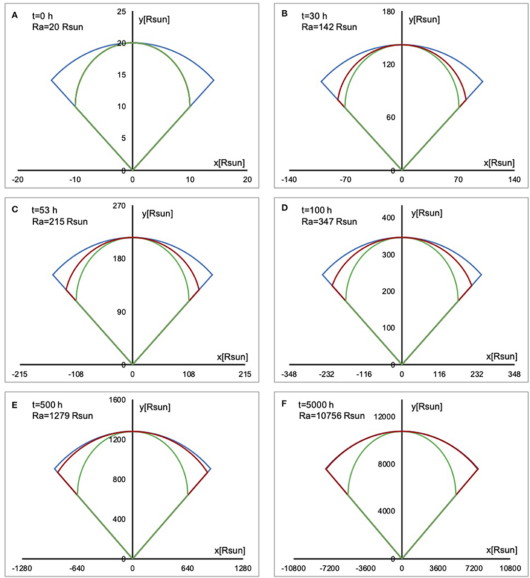
Figure 1. The differences between the fronts at six arbitrarily chosen time-steps for the three DBM tools: basic 1D DBM (the concentric leading edge, blue), advanced 2D DBM with self-similar cone geometry (green), and the advanced 2D DBM with flattening cone geometry (red). The subplots show the position of the leading edge in the XY coordinate system (i.e., the solar equatorial plane). The heliospheric distance of the apex, Ra, is highlighted in each time-step. The following DBM parameters were used to create the plots: initial CME speed of 1,000 kms−1, initial distance of 20R⊙, γ of 0.2·10−7km−1, and solar wind speed w of 450kms−1.
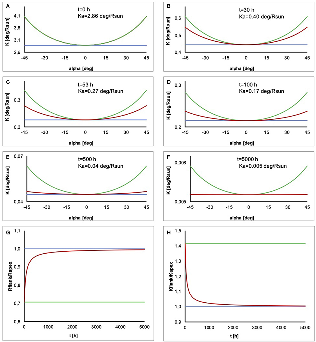
Figure 2. The differences between the curvatures of the fronts at different time-steps for the three DBM tools: basic 1D DBM (the concentric leading edge, blue), advanced 2D DBM with self-similar cone geometry (green), and the advanced 2D DBM with flattening cone geometry (red). The time-steps and DBM parameters correspond to those used in Figure 1. The subplots (A–F) show how the curvature K along the leading edge behaves in time. The curvature at the apex, Ka, is highlighted in each time-step. The subplot (G) shows how the ratio of the flank heliospheric distance and the apex heliospheric distance (Rf/Ra) evolves in time, whereas subplot (H) shows how the ratio of the curvature at the flank and at the apex (Kf/Ka) evolves in time.
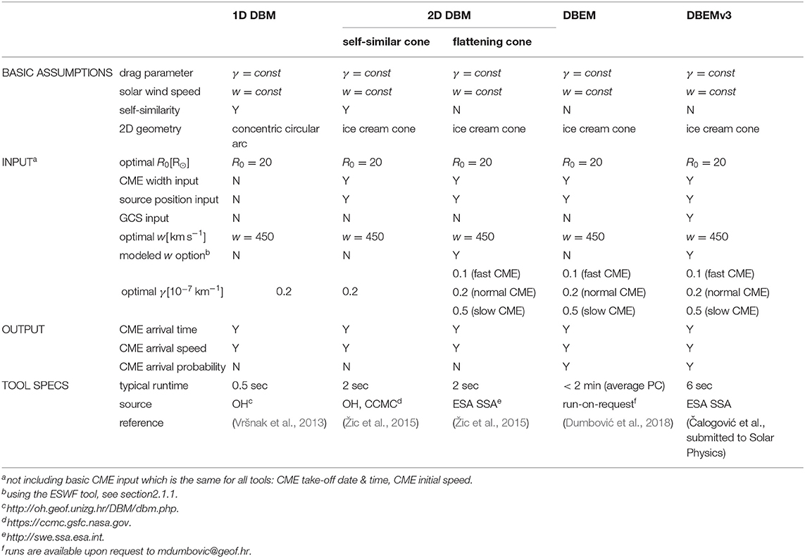
Table 1. Comparison of DBM tools.
The advanced form of the DBM was formulated by Žic et al. (2015), who applied a 2D cone geometry to the basic 1D DBM solutions given in Equation (2). The cone geometry was selected as it is a standard geometry used in heliospheric models, such as ENLIL (Odstrcil et al., 2004) or EUHFORIA (Pomoell and Poedts, 2018), and therefore, their input would be suitable for use in DBM as well. The cone angular dependence is introduced in DBM in the following form:
where R0 and v0 are distance and speed of the plasma element at the CME apex, ω is the half-width of the cone (i.e., of the CME opening angle), and α is the opening angle corresponding to the plasma element in question. Depending on the applications of the cone-geometry given by Equation (4) to the basic 1D DBM solutions given in Equation (2), two different evolutions of the CME leading edge are possible, namely self-similar cone evolution and the flattening cone evolution.
The self-similar evolution of the cone leading edge is obtained assuming that the CME front does not change its shape, i.e., when the DBM solutions for a plasma element after time t at the angular distance α from the apex at the leading edge is given by:
where R0(t) and v0(t) are given by Equation (2). The self-similar cone leading edge is compared to the concentric geometry as well as the flattening cone leading edge in Figures 1, 2. This has been adopted by the online DBM tool that runs on the Hvar Observatory webpage2, as well as the Community Coordinated Modeling Centre (CCMC)3. Since the tool does implement information on the CME angular extent and its direction, it also provides information of whether or not the CME hits the target.The basic assumptions, input, output, and tool specifications are given in the third column of Table 1.
The flattening cone leading edge evolution is obtained by propagating each plasma element of the CME leading edge independently, using the CME 2D cone geometry given by Equation (4) as the initial leading edge. The DBM solutions for a plasma element after time t at the angular distance α from the apex at the leading edge is given by:
where R0(α) and v0(α) are given by Equation (4). The flattening cone leading edge is also shown in Figures 1, 2 and similarly as 2D self-similar DBM provides information whether or not the CME hits the target. The basic assumptions, input, output, and tool specifications are given in the fourth column of Table 1.
To summarize, three different geometries of the CME leading edge (CME front) are considered in DBM tools: concentric arc, self-similarly evolving cone, and flattening cone. The differences between the fronts and their evolution for the three tools described above are shown in Figure 1 for halfwidth < 90° at several arbitrarily chosen time-steps. The x subplots (a–f) show the position of the leading edge in the XY coordinate system for six different time-steps. It can be seen that initially (at t = 0) we differentiate only 2 geometries, the concentric arc and the cone geometry leading edge. Although the initial shape of the flattening cone leading edge is that of a 2D cone, at t > 0, the shape of the leading edge starts to increasingly deviate from the initial cone shape. This is because each plasma element of the leading edge is propagated independently using different initial parameters. A plasma element at the flank will have a lower value of the initial speed than, e.g., a plasma element at the apex and will therefore experience less drag if the CME is faster than the solar wind and more drag if the CME is slower than the solar wind. Since the drag will not act equally on each plasma element across the leading edge, the evolution of the leading edge will not be self-similar. Instead, as can be seen in Figure 1, during the evolution, the leading edge will gradually change from the initial cone shape toward a flatter shape.
This can be seen more prominently in Figure 2, which shows the time-evolution of the curvature of the CME leading edge with respect to the center of the Sun, calculated as K = ΔΘ/ΔL, where ΔΘ = |Θ1 − Θ2| is the angular distance and is the corresponding arc length of the curve in polar coordinates. Note that thus defined K does not correspond to the standard mathematical term curvature, which is defined with respect to the center of the circle and thus remains always constant across the circular arc. Instead, we define quantity K to differ between the concentric arc and self-similar cone in the polar coordinates with the origin at the center of the Sun. We can see that K of the concentric arc is constant across the leading edge, whereas K of the 2D cone at the apex is identical to that of the concentric arc but increases toward the flanks. However, the difference in K between the flank and the apex remains constant in time for a self-similarly evolving cone front, whereas it reduces for the flattening cone front.
The last two subplots of Figure 2 show the ratio of the flank distance to the apex distance, Rf/Ra, and the ratio of the curvature at the flank and at the apex, Kf/Ka. For self-similarly evolving fronts, Rf/Ra and Kf/Ka are constant and, in the specific case of a concentric leading edge, both equal to 1 (values at the flank are equal to the values at the apex). We see that the apex evolves identically in all three cases. For a self-similarly evolving cone, Rf/Ra and Kf/Ka remain constant. For the flattening cone, Rf/Ra and Kf/Ka are not constant, as the Rf/Ra increases and Kf/Ka decreases in time, both approaching the values for the concentric leading edge. It should be noted, however, that they never actually reach the values for the concentric leading edge. This is because, although the flank experiences different drag than the apex, it is slower than the apex. The difference between Rf and Ra is increasing, converging to a certain value, as the drag eventually adjusts the speed of both the apex and the flank to the ambient solar wind speed. As the distance from the Sun increases, the difference between Rf and Ra becomes very small compared to values of Rf and Ra; therefore, Rf/Ra seems to converge to 1, although mathematically it will never reach it and the flattening cone will never truly become a concentric arc. It is also important to note that, for a halfwidth of 90°, all three fronts are semi-circles with the origin at the center of the Sun and thus evolve identically, as the concentric arc.
2.3. The Ensemble Versions of the DBM
As noted in section 1, DBMs are computationally efficient and thus widely used in probabilistic/ensemble modeling approaches. Ensemble forecasting takes into account the errors and uncertainties of the input to quantify the resulting uncertainties in the model predictions. The variability of an observational input is introduced by making an ensemble, i.e., sets of CME observations to calculate a distribution of predictions and forecast the confidence in the likelihood of the prediction. This can be achieved in two ways: (1) by taking independently built sets of CME observations (e.g., as provided by different observers) or (2) by creating sets of CME observations (by, e.g., using measurements and error estimations provided by a single observer). These two ensemble options were adopted in the Drag-based ensemble model (DBEM) (Dumbović et al., 2018) and DBEMv3 web tool (Čalogović et al., submitted to Solar Physics), respectively, which both use 2D DBM with flattening cone as a background physical model. The output of both tools is the probability of arrival, which is calculated as the ratio of the number of runs that predict a hit and total number of runs. Based on the runs that predict a hit, distributions of arrival time and speed are generated, where the calculated medians represent the likeliest arrival time and speed, and the uncertainty range is given by 95% confidence interval. Note that initially there was a DBEMv2, which was replaced by a more advanced DBEMv3.
For a single CME, DBEM uses an ensemble of n measurements of the same CME, which may not be mutually related in any way (e.g., it might be obtained by different observers, different methods, or even measurements from different instruments). Each ensemble member has the same weight. Moreover, there is no assumption that the CME measurements of a particular CME, i.e., ensemble member, are independent of each other or that their spread in values follow a certain distribution. The variability of solar wind speed, w, and drag parameter, γ, are taken into account by producing m of their synthetic values. These synthetic values are combined with an ensemble of n CME measurements to give a final ensemble of n·m2 members as an input, which, after n·m2 runs, produces a distribution of n·m2 calculated CME transit times and arrival speeds. The synthetic values for w and γ are produced by assuming that their real measurements follow a normal distribution with a mean value and SD serving as the model input. A cumulative standard normal distribution is then generated, defined on an interval [0, m − 1], where m is the number of synthetic measurements, also used as the model input. The m values which correspond to the integer values of the cumulative standard normal distribution are selected as synthetic measurements. This way, for identical distribution and m, the selection always results in an identical set of synthetic values, which include the tips of the distribution tail. Therefore, for small m the distribution of chosen synthetic measurements is too heavily weighed to the tail compared to the normal distribution, and larger m is needed for synthetic measurements to be weighted properly, m > 15 (Dumbović et al., 2018). The basic assumptions, input, output, and tool specifications of DBEM are given in the fifth column of Table 1.
In DBEMv3, the CME ensemble is not produced by the observer, but the tool. Observational input values and uncertainties are provided for the CME input as well as for w and γ, from which the tool generates m ensemble members. Each ensemble member is produced by randomly picking one value for each input parameter, assuming that it follows a normal distribution with the observational input value as mean and SD derived from uncertainty (uncertainty = 3σ). Due to this randomness (which cannot be controlled), the ensemble is not likely to be identical each time an identical input is used, which produces small differences in the output of the model for different runs using identical input. However, for large ensembles, m > 10, 000, the differences of the output are negligible (see documentation of the DBEMv3 at ESA/SSA4 as well as Čalogović et al., submitted to Solar Physics). The basic assumptions, input, output, and tool specifications of DBEMv3 are given in the last column of Table 1.
We note that, in the DBEMv3, the CME input parameters are considered to be independent of each other and therefore, the procedure is somewhat similar to error propagation. In DBEM, the CME parameters within one measurement set are not necessarily independent of each other, CME sets are independent of each other. This is important due to the nature of the model input used, i.e., obtaining CME input from coronagraphic measurements. Coronagraphs only display a projection of a 3D structure. Therefore, in order to derive parameters of a 3D CME, some assumptions need to be made on the CME geometry. These assumptions, as well as their applications can vary from observer-to-observer and result in CME measurement sets where the distribution of single parameter variability may differ substantially from the normal distribution. A single observer, on the other hand, is more likely to provide CME measurements with errors that follow a normal distribution. While a single observer is more likely to bias the mean of the normal distribution of an input parameter and thus introduce errors, we note that, in the near-real-time forecasting, where a quick estimation of the CME input is needed, DBEMv3 is more applicable, since it uses input provided by only one observer/method.
3. Running the DBM Tools: Example Event
We demonstrate the performance of DBM tools described in section 2 by running all the tools using the same example event. As the example event, we chose a previously studied CME that erupted on April 3, 2010 and hit Earth on April 5, 2010 (e.g., Möstl et al., 2010; Wood et al., 2011; Rodari et al., 2018). This event can be found in the SOHO/LASCO CME catalog 5, where it is listed as a halo with the first appearance in LASCO-C2 on April 3, 2010 at 10:33 UT. In order to reconstruct the flux rope structure of the CME, we used the graduated cylindrical shell (GCS) model (Thernisien et al., 2006, 2009; Thernisien, 2011).
Graduated cylindrical shell is a geometrical model used to describe the flux rope structure of the CME to study its three-dimensional morphology, position, and kinematics. The flux rope is approximated with a self-similarly expanding hollow croissant originating from the center of the Sun, where the legs are conical and cross-section circular and the front is pseudo-circular. The croissant is fully defined by six GCS parameters: (1) longitude, (2) latitude, (3) height corresponding to the apex of the croissant, (4) the tilt of the croissant axis to the solar equatorial plane, (5) the croissant half-angle measured between the apex and the central axis of its leg, and (6) the “aspect ratio” (i.e., the sine of the angle defining the “thickness” of the croissant leg). The GCS parameters were obtained by fitting its 2D projections to the respective coronagraphic images, where at least two different vantage points are needed to constrain the geometry (for further details on GCS, see Thernisien et al., 2006, 2009; Thernisien, 2011).
To perform the reconstruction, we used coronagraph images taken by SECCHI/COR2 (Howard et al., 2008) onboard STEREO-A and B, as well as LASCO-C3 (Brueckner et al., 1995) onboard SOHO spacecraft on April 3, 2010 at 10:54 UT. Furthermore, the GCS reconstruction was done in four consecutive time-steps, following the CME leading edge while changing only the height parameter, i.e., assuming self-similar expansion. Based on these four measurements, a CME linear speed of 920kms−1 was estimated. The GCS best fit parameters and linear speed are given in the second column of Table 2 and the reconstruction is shown in Figure 3.
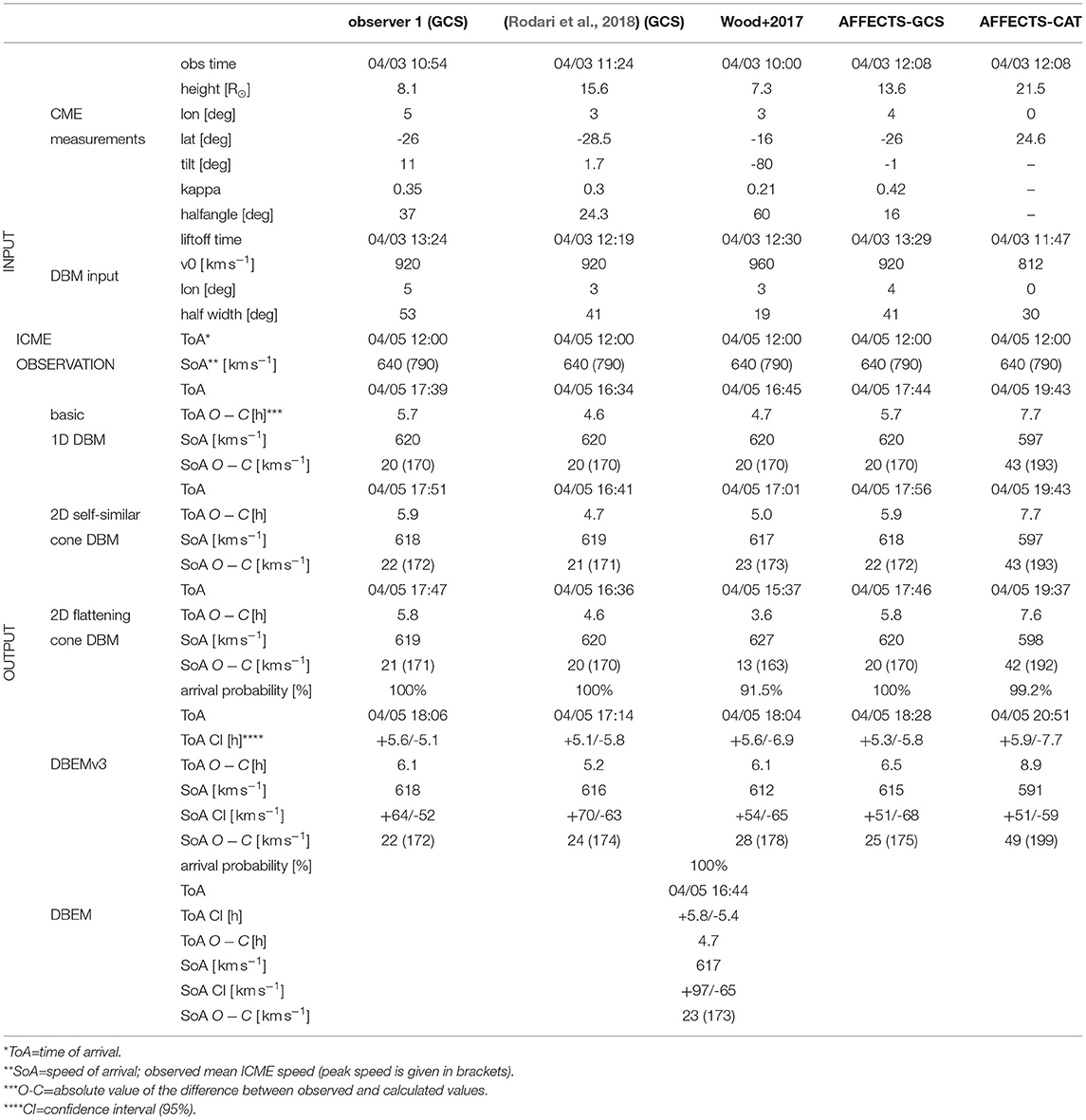
Table 2. CME measurements and the corresponding DBM input and output for the April 3rd 2010 CME for 5 different observers using 3 different methods.
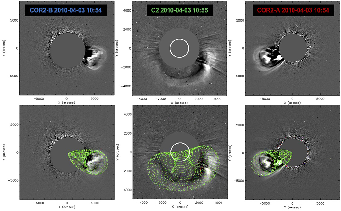
Figure 3. The CME of April 3, 2010, observed in running difference images in STEREO/COR2 and SOHO/LASCO coronagraphs and the GCS reconstruction of the CME (green mesh).
Based on the results of the GCS reconstruction, we derived the input for the DBM tools (see column 4 in Table 2). Using the CME linear speed, we extrapolated the CME apex to R0 = 20R⊙ assuming constant speed, which is taken as the initial CME speed, v0. The CME angular extent (i.e., CME angular half width, λ) in the solar equatorial plane was estimated based on the GCS-derived tilt, as well as the GCS face-on and edge-on widths, as described by Dumbović et al. (2019) and adopted in DBEMv3. The projection of the GCS reconstructed CME in the solar equatorial plane is shown in Figure 4, as well as the calculated CME angular extent and the positions of the spacecraft. We can see that, due to relatively small tilt and large half-angle, the angular extent of the CME is quite large. In addition, we can see that the direction of the apex (given by the longitude of the CME source region, ϕCME) is very close to the Sun-Earth line. We next ran DBM tools for the input obtained from the GCS reconstruction (bottom rows of Table 2). In order to run DBEM, for which different sets of CME measurements are needed as input, we utilized measurements from previous studies on this event (Wood et al., 2017; Rodari et al., 2018) and from online catalogs provided by the Advanced Forecast For Ensuring Communications Through Space (AFFECTS)6 catalogs. We used CME input provided by the AFFECTS-GCS database and the AFFECTS-CAT database, where the latter is obtained with the CME Analysis Tool (CAT) modeling technique developed by Millward et al. (2013). We also ran all other DBM tools for these various CME inputs [as given in columns (5-8)]. The DBM input for these CME measurements was derived the same way as for the GCS reconstruction performed here. The CME speed for AFFECTS-GCS catalog was assumed to be the same as that in other two GCS reconstructions. CME measurements provided by five different observers using three different measurement methods, as well as the corresponding five DBM inputs the are given in Table 2.
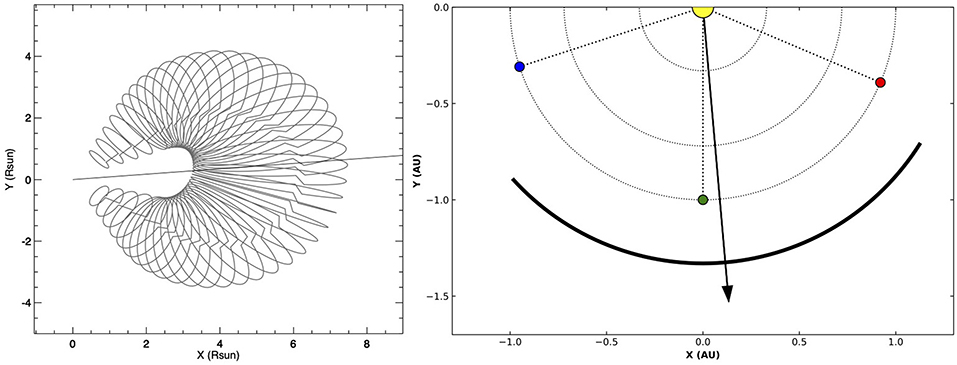
Figure 4. (Left) The projection of the GCS croissant of the on April 3, 2010, CME in the XY plane of the Heliocentric Earth Equatorial (HEEQ) coordinate system (i.e., plane of the solar equator). The direction of the apex is marked by a solid black line. (Right) The direction and angular extent of the April 3rd 2010 CME (black arrow and black arc, respectively) and the positions of the three spacecrafts in the HEEQ coordinate system at the CME liftoff time: STEREO-B (blue), SOHO (green), and STEREO-A (red).
The inner boundary, the drag parameter, the solar wind speed, and target distance are the same for each of the five DBM inputs and are R0 = 20R⊙, γ = 0.2·10−7km−1, w = 450kms−1, and Rtarget = 1 au, respectively. In DBEM, 15 synthetic values of γ and w were used within the uncertainty ranges ±0.1·10−7km−1 and ±50kms−1, respectively. In DBEMv3, default uncertainty ranges of the tool were used: ±30 min, ±0.1·10−7km−1, ±50kms−1, ±200kms−1, ±15°, and ±30° for lift-off time, γ, w, v0, λ, and ϕCME, respectively, and 10,000 runs were performed to obtain the results. It can be seen in Table 2 that the difference in the output of different DBM tools is very similar for all DBM tools that use a single input set (basic 1D DBM, 2D self-similar DBM, 2D flattening cone DBM, and DBEMv3). This is because the direction of the apex is very close to the direction of the target, i.e., the CME is likely to hit the target close to the apex, where all geometries evolve similarly. This is also the reason for very high arrival probability, given that the most of the input sets consider a relatively wide CME. The input set derived based on measurements given by Wood et al. (2017) in their study is the only one yielding a DBEMv3 arrival probability < 100%, because the estimated CME half width is low compared to the uncertainty. The difference of the output is more prominent between different input sets than between different tools, with the exception of DBEM, which shows slightly different results compared to other tools. This is because, unlike other DBM tools, DBEM does not use a single input but takes into account the variability of different input sets.
The last two rows of Table 2 show the observational results for the CME arrival, which are based on the CME-ICME association made by Möstl et al. (2010) and the arrival time and speed values provided by the ICME catalog of Richardson and Cane (2010)7, where the mean ICME speed is taken as the arrival speed and the ICME start (not the start of the disturbance) is taken as the arrival time. Measured ICME peak speed is also given for reference. We can see that, all DBM outputs in Table 2 overestimate arrival time by a couple of hours and underestimate arrival speed by couple of tens of kms−1, which indicated that the drag was overestimated. Indeed, as this is a fast event, 2D flattening cone DBM, DBEM, and DBEMv3 would suggest the γ = 0.1·10−7km−1 option. Running DBEMv3 and DBEM with γ = 0.1·10−7km−1 and keeping other input identical, as given in Table 2 yield arrival times 2010-04-05 13:20 and 2010-04-05 11:50 UT, respectively, i.e., very close to the observed arrival time. The DBEMv3 and DBEM outputs, for arrival speed are 705kms−1 for both, which is closer to the observed ICME peak speed instead of the ICME mean speed.
4. Discussion and Conclusion
The basic DBM equations (Equations 1, 2) describe CME propagation in a simple, physics-based and analytical way. Therefore, even when CME geometry is included (2D DBM) and in the ensemble mode, the model runs very quickly (Table 1). With the development of different tools and their performance analysis, optimized DBM parameters (e.g., initial distance, solar wind speed, and drag parameter) have been established, which are offered as default parameters in the DBM tools (Table 1). This makes the tools very easy to use, even for the unexperienced users. On the other hand, the tools allow customized input for more experienced users (as described in section 2.1.1). Therefore, DBM tools are simple to use and computationally efficient, which is their main advantage, compared to numerical MHD models.
DBM tools offer three different geometries, which identically describe the propagation of the CME apex, but differ in the description of the CME flanks, and might therefore differ in the applicability. For instance, both 2D DBM tools assume initial cone geometry; however, one propagates it in a self-similar manner, whereas the other does not. Therefore, it is reasonable to assume that 2D self-similar DBM might be more suitable for CMEs with (near) the self-similar expansion. This might be the case with slower CMEs, which show more symmetric in situ profiles (Masías-Meza et al., 2016). Since they propagate with speeds closer to the solar wind speed, they experience less drag. On the other hand, 2D flattening cone DBM might be more suitable for very fast CMEs, which show quite asymmetric in situ profiles (Masías-Meza et al., 2016), indicating non-self similar expansion. They propagate with speeds much larger than the solar wind speed and thus experience more drag. The non-self similar vs. self-similar evolution might become even more important for considerations of 3D geometries. It is important to note that 2D flattening cone DBM does not consider change of the front in a manner that the flanks catch-up or overtake the apex. It is a purely geometrical effect, a change from a highly-curved cone geometry toward a less-curved concentric-arc-like geometry, and is not related to, e.g., non-homogeneous drag or internal forces that might cause the “pancaking effect” (e.g., Cargill et al., 1994). The cone geometry is also suitable to describe the propagation of a CME driven shock, which is typically faster and stronger at the nose compared to flanks (e.g., Neugebauer, 2013); thus, the flanks are “delayed” with respect to the nose. On the other hand, for a freely propagating shock, assuming it propagates in a homogeneous medium, a concentric arc geometry might be more suitable. As demonstrated on an example event, for CME propagation near the apex, all geometries and, therefore, all DBM tools show similar results (provided that the CME input is the same, see Table 2).
The ensemble options of the DBM provide a more comprehensive prediction compared to the other three tools, as they additionally calculate arrival probability and confidence interval of the arrival time and speed. In addition, although they rely on a large number of DBM runs (> 1, 000), they are still computationally inexpensive (Table 1). Therefore, they are quite useful from the aspect of space weather forecast and its evaluation. Since there is a difference in the implementation of the CME input in DBEM and DBEMv3, their applicability may also differ. The DBEMv3 tool is much faster and only needs input from one observer; thus, it is easy to use in near-real time forecasts. On the other hand, DBEM may use various CME input sets, provided by different observers, different methods, or even different instruments, and may thus be more suitable for evaluation purposes.
To summarize, this study provides an overview of the assumptions, applications, and performance of the five DBM tools developed at Hvar Observatory. It is important to note that, although these tools were developed sequentially and therefore each more recent tool contains improvements compared to the older version, the older versions still have their applicability.
Data Availability Statement
The original contributions presented in the study are included in the article/supplementary material, further inquiries can be directed to the corresponding author/s.
Author Contributions
MD, MT and JC contributed to the initial conception of the paper. MD, with the help of KM, wrote the main draft and prepared figures, having discussion on analysis with other co-authors. All of the authors have read the paper and approved its final version.
Conflict of Interest
The authors declare that the research was conducted in the absence of any commercial or financial relationships that could be construed as a potential conflict of interest.
Acknowledgments
MD acknowledges support by the Croatian Science Foundation under the project IP-2020-02-9893 (ICOHOSS) and International Space Science Institute (ISSI) team Understanding Our Capabilities in Observing and Modeling Coronal Mass Ejections, led by C. Verbeke and M. Mierla. JC, BV, and DS acknowledge support by the Croatian Science Foundation under the project 7549 (MSOC). KM acknowledges support by the Croatian Science Foundation in the scope of the Young Researchers Career Development Project Training New Doctoral Students. This research has received financial support from the European Union's Horizon 2020 research and innovation program under grant agreement no. 824135 (SOLARNET).
Footnotes
1. ^http://oh.geof.unizg.hr/DBM/dbm.php.
2. ^http://oh.geof.unizg.hr/DBM/dbm.php.
3. ^https://ccmc.gsfc.nasa.gov.
5. ^https://cdaw.gsfc.nasa.gov/CME_list/.
6. ^http://www.affects-fp7.eu/home/.
7. ^http://www.srl.caltech.edu/ACE/ASC/DATA/level3/icmetable2.htm.
References
Amerstorfer, T., Hinterreiter, J., Reiss, M. A., Möstl, C., Davies, J. A., Bailey, R. L., et al. (2021). Evaluation of CME arrival prediction using ensemble modeling based on heliospheric imaging observations. Space Weather. 19:e02553. doi: 10.1029/2020SW002553
Amerstorfer, T., Möstl, C., Hess, P., Temmer, M., Mays, M. L., Reiss, M. A., et al. (2018). Ensemble prediction of a Halo coronal mass ejection using heliospheric imagers. Space Weather 16, 784–801. doi: 10.1029/2017SW001786
Bein, B. M., Temmer, M., Vourlidas, A., Veronig, A. M., and Utz, D. (2013). The height evolution of the “True” coronal mass ejection mass derived from STEREO COR1 and COR2 observations. Astrophys. J. 768:31. doi: 10.1088/0004-637X/768/1/31
Bothmer, V., and Schwenn, R. (1998). The structure and origin of magnetic clouds in the solar wind. Ann. Geophys. 16, 1–24. doi: 10.1007/s00585-997-0001-x
Brueckner, G. E., Howard, R. A., Koomen, M. J., Korendyke, C. M., Michels, D. J., Moses, J. D., et al. (1995). The large angle spectroscopic coronagraph (LASCO). Solar Phys. 162, 357–402.
Cargill, P. J. (2004). On the aerodynamic drag force acting on interplanetary coronal mass ejections. Solar Phys. 221, 135–149. doi: 10.1023/B:SOLA.0000033366.10725.a2
Cargill, P. J., Chen, J., Spicer, D. S., and Zalesak, S. T. (1994). “The deformation of flux tubes in the solar wind with applications to the structure of magnetic clouds and CMEs,” in Solar Dynamic Phenomena and Solar Wind Consequences, the Third SOHO Workshop, Vol. 373, ed J. J. Hunt (Estes Park, CO: ESA Special Publication), 291.
Cargill, P. J., Chen, J., Spicer, D. S., and Zalesak, S. T. (1996). Magnetohydrodynamic simulations of the motion of magnetic flux tubes through a magnetized plasma. J. Geophys. Res. 101, 4855–4870. doi: 10.1029/95JA03769
Colaninno, R. C., and Vourlidas, A. (2009). First determination of the true mass of coronal mass ejections: a novel approach to using the Two STEREO viewpoints. Astrophys. J. 698, 852–858. doi: 10.1088/0004-637X/698/1/852
Démoulin, P., Nakwacki, M. S., Dasso, S., and Mandrini, C. H. (2008). Expected in situ velocities from a hierarchical model for expanding interplanetary coronal mass ejections. Solar Phys. 250, 347–374. doi: 10.1007/s11207-008-9221-9
Desai, R. T., Zhang, H., Davies, E. E., Stawarz, J. E., Mico-Gomez, J., and Iváñez-Ballesteros, P. (2020). Three-dimensional simulations of solar wind preconditioning and the 23 July 2012 interplanetary coronal mass ejection. Solar Phys. 295:130. doi: 10.1007/s11207-020-01700-5
Dissauer, K., Veronig, A. M., Temmer, M., and Podladchikova, T. (2019). Statistics of coronal dimmings associated with coronal mass ejections. II. Relationship between coronal dimmings and their associated CMEs. Astrophys. J. 874:123. doi: 10.3847/1538-4357/ab0962
Dryer, M., Fry, C. D., Sun, W., Deehr, C., Smith, Z., Akasofu, S.-I., et al. (2001). Prediction in real time of the 2000 july 14 heliospheric shock wave and its companions during the ‘Bastille' Epoch*. Solar Phys. 204, 265–284. doi: 10.1023/A:1014200719867
Dumbović, M., Čalogović, J., Vršnak, B., Temmer, M., Mays, M. L., Veronig, A., et al. (2018). The drag-based ensemble model (DBEM) for coronal mass ejection propagation. Astrophys. J. 854:180. doi: 10.3847/1538-4357/aaaa66
Dumbović, M., Guo, J., Temmer, M., Mays, M. L., Veronig, A., Heinemann, S. G., et al. (2019). Unusual plasma and particle signatures at mars and STEREO-A related to CME–CME interaction. Astrophys. J. 880:18. doi: 10.3847/1538-4357/ab27ca
Gopalswamy, N., Lara, A., Lepping, R. P., Kaiser, M. L., Berdichevsky, D., and St. Cyr, O. C. (2000). Interplanetary acceleration of coronal mass ejections. Geophys. Res. Lett. 27, 145–148. doi: 10.1029/1999GL003639
Gopalswamy, N., Lara, A., Yashiro, S., Kaiser, M. L., and Howard, R. A. (2001). Predicting the 1-AU arrival times of coronal mass ejections. J. Geophys. Res. 106, 29207–29218. doi: 10.1029/2001JA000177
Guo, J., Dumbović, M., Wimmer-Schweingruber, R. F., Temmer, M., Lohf, H., Wang, Y., et al. (2018). Modeling the evolution and propagation of 10 september 2017 CMEs and SEPs arriving at mars constrained by remote sensing and in situ measurement. Space Weather 16, 1156–1169. doi: 10.1029/2018SW001973
Hess, P., and Zhang, J. (2014). Stereoscopic study of the kinematic evolution of a coronal mass ejection and its driven shock from the sun to the earth and the prediction of their arrival times. Astrophys. J. 792:49. doi: 10.1088/0004-637X/792/1/49
Hess, P., and Zhang, J. (2015). Predicting CME ejecta and sheath front arrival at L1 with a data-constrained physical model. Astrophys. J. 812:144. doi: 10.1088/0004-637X/812/2/144
Howard, R. A., Moses, J. D., Vourlidas, A., Newmark, J. S., Socker, D. G., Plunkett, S. P., et al. (2008). Sun earth connection coronal and heliospheric investigation (SECCHI). Space Sci. Rev. 136, 67–115. doi: 10.1007/s11214-008-9341-4
Howard, T. A., and Tappin, S. J. (2009). Interplanetary coronal mass ejections observed in the heliosphere: 1. Review of theory. Space Sci. Rev. 147, 31–54. doi: 10.1007/s11214-009-9542-5
Kay, C., and Gopalswamy, N. (2018). The effects of uncertainty in initial CME input parameters on deflection, rotation, Bz, and arrival time predictions. J. Geophys. Res. 123, 7220–7240. doi: 10.1029/2018JA025780
Kay, C., Mays, M. L., and Verbeke, C. (2020). Identifying critical input parameters for improving drag-based CME arrival time predictions. Space Weather 18:e02382. doi: 10.1029/2019SW002382
Kilpua, E., Koskinen, H. E. J., and Pulkkinen, T. I. (2017). Coronal mass ejections and their sheath regions in interplanetary space. Liv. Rev. Solar Phys. 14:5. doi: 10.1007/s41116-017-0009-6
Liu, J., Ye, Y., Shen, C., Wang, Y., and Erdélyi, R. (2018). A new tool for CME arrival time prediction using machine learning algorithms: CAT-PUMA. Astrophys. J. 855:109. doi: 10.3847/1538-4357/aaae69
Manchester, W., Kilpua, E. K. J., Liu, Y. D., Lugaz, N., Riley, P., Török, T., et al. (2017). The physical processes of CME/ICME evolution. Space Sci. Rev. 212, 1159–1219. doi: 10.1007/s11214-017-0394-0
Maričić, D., Vršnak, B., Stanger, A. L., Veronig, A. M., Temmer, M., and Roša, D. (2007). Acceleration phase of coronal mass ejections: II. Synchronization of the energy release in the associated flare. Solar Phys. 241, 99–112. doi: 10.1007/s11207-007-0291-x
Masías-Meza, J. J., Dasso, S., Démoulin, P., Rodriguez, L., and Janvier, M. (2016). Superposed epoch study of ICME sub-structures near Earth and their effects on Galactic cosmic rays. Astron. Astrophys. 592:A118. doi: 10.1051/0004-6361/201628571
Mikić, Z., Linker, J. A., Schnack, D. D., Lionello, R., and Tarditi, A. (1999). Magnetohydrodynamic modeling of the global solar corona. Phys. Plasmas 6, 2217–2224. doi: 10.1063/1.873474
Millward, G., Biesecker, D., Pizzo, V., and de Koning, C. A. (2013). An operational software tool for the analysis of coronagraph images: determining CME parameters for input into the WSA-Enlil heliospheric model. Space Weather 11, 57–68. doi: 10.1002/swe.20024
Möstl, C., Amerstorfer, T., Palmerio, E., Isavnin, A., Farrugia, C. J., Lowder, C., et al. (2018). Forward modeling of coronal mass ejection flux ropes in the inner heliosphere with 3DCORE. Space Weather 16, 216–229. doi: 10.1002/2017SW001735
Möstl, C., Rollett, T., Frahm, R. A., Liu, Y. D., Long, D. M., Colaninno, R. C., et al. (2015). Strong coronal channelling and interplanetary evolution of a solar storm up to Earth and Mars. Nat. Commun. 6:7135. doi: 10.1038/ncomms8135
Möstl, C., Temmer, M., Rollett, T., Farrugia, C. J., Liu, Y., Veronig, A. M., et al. (2010). STEREO and Wind observations of a fast ICME flank triggering a prolonged geomagnetic storm on 5-7 April 2010. Geophys. Res. Lett. 37:L24103. doi: 10.1029/2010GL045175
Napoletano, G., Forte, R., Moro, D. D., Pietropaolo, E., Giovannelli, L., and Berrilli, F. (2018). A probabilistic approach to the drag-based model. J. Space Weather Space Clim. 8:A11. doi: 10.1051/swsc/2018003
Neugebauer, M. (2013). Propagating shocks. Space Sci. Rev. 176, 125–132. doi: 10.1007/s11214-010-9707-2
Odstrcil, D., Riley, P., and Zhao, X. P. (2004). Numerical simulation of the 12 May 1997 interplanetary CME event. J. Geophys. Res. 109:A02116. doi: 10.1029/2003JA010135
Paouris, E., Čalogović, J., Dumbović, M., Mays, M. L., Vourlidas, A., Papaioannou, A., et al. (2021). Propagating conditions and the time of ICME arrival: a comparison of the effective acceleration model with ENLIL and DBEM models. Solar Phys. 296:12. doi: 10.1007/s11207-020-01747-4
Paouris, E., and Mavromichalaki, H. (2017). Effective acceleration model for the arrival time of interplanetary shocks driven by coronal mass ejections. Solar Phys. 292:180. doi: 10.1007/s11207-017-1212-2
Pomoell, J., and Poedts, S. (2018). EUHFORIA: European heliospheric forecasting information asset. J. Space Weather Space Clim. 8:A35. doi: 10.1051/swsc/2018020
Reiss, M. A., Temmer, M., Veronig, A. M., Nikolic, L., Vennerstrom, S., Schöngassner, F., et al. (2016). Verification of high-speed solar wind stream forecasts using operational solar wind models. Space Weather 14, 495–510. doi: 10.1002/2016SW001390
Richardson, I. G., and Cane, H. V. (2010). Near-earth interplanetary coronal mass ejections during solar cycle 23 (1996 - 2009): catalog and summary of properties. Solar Phys. 264, 189–237. doi: 10.1007/s11207-010-9568-6
Riley, P., Mays, M. L., Andries, J., Amerstorfer, T., Biesecker, D., Delouille, V., et al. (2018). Forecasting the arrival time of coronal mass ejections: analysis of the CCMC CME scoreboard. Space Weather 16, 1245–1260. doi: 10.1029/2018SW001962
Rodari, M., Dumbović, M., Temmer, M., Holzknecht, L., and Veronig, A. (2018). 3D reconstruction and interplanetary expansion of the 2010 April 3rd CME. Central Eur. Astrophys. Bull. 42:11.
Rollett, T., Möstl, C., Isavnin, A., Davies, J. A., Kubicka, M., Amerstorfer, U. V., et al. (2016). ElEvoHI: a novel CME prediction tool for heliospheric imaging combining an elliptical front with drag-based model fitting. Astrophys. J. 824:131. doi: 10.3847/0004-637X/824/2/131
Rotter, T., Veronig, A. M., Temmer, M., and Vršnak, B. (2012). Relation between coronal hole areas on the sun and the solar wind parameters at 1 AU. Solar Phys. 281, 793–813. doi: 10.1007/s11207-012-0101-y
Sachdeva, N., Subramanian, P., Colaninno, R., and Vourlidas, A. (2015). CME propagation: where does aerodynamic drag 'Take Over'? Astrophys. J. 809:158. doi: 10.1088/0004-637X/809/2/158
Sachdeva, N., Subramanian, P., Vourlidas, A., and Bothmer, V. (2017). CME dynamics using STEREO and LASCO observations: the relative importance of lorentz forces and solar wind drag. Solar Phys. 292:118. doi: 10.1007/s11207-017-1137-9
Sheeley, N. R., Walters, J. H., Wang, Y.-M., and Howard, R. A. (1999). Continuous tracking of coronal outflows: two kinds of coronal mass ejections. J. Geophys. Res. 104, 24739–24768. doi: 10.1029/1999JA900308
Siscoe, G., and Schwenn, R. (2006). CME disturbance forecasting. Space Sci. Rev. 123, 453–470. doi: 10.1007/978-0-387-45088-9_17
Sudar, D., Vršnak, B., and Dumbović, M. (2016). Predicting coronal mass ejections transit times to Earth with neural network. Mon. Not. R. Astron. Soc. 456, 1542–1548. doi: 10.1093/mnras/stv2782
Takahashi, T., and Shibata, K. (2017). Sheath-accumulating propagation of interplanetary coronal mass ejection. Astrophys. J. Lett. 837:L17. doi: 10.3847/2041-8213/aa624c
Temmer, M. (2016). Kinematical properties of coronal mass ejections. Astron. Nachr. 337:1010. doi: 10.1002/asna.201612425
Temmer, M., and Nitta, N. V. (2015). Interplanetary propagation behavior of the fast coronal mass ejection on 23 July 2012. Solar Phys. 290, 919–932. doi: 10.1007/s11207-014-0642-3
Temmer, M., Reiss, M. A., Nikolic, L., Hofmeister, S. J., and Veronig, A. M. (2017). Preconditioning of interplanetary space due to transient CME disturbances. Astrophys. J. 835:141. doi: 10.3847/1538-4357/835/2/141
Temmer, M., Vršnak, B., and Veronig, A. M. (2007). Periodic appearance of coronal holes and the related variation of solar wind parameters. Solar Phys. 241, 371–383. doi: 10.1007/s11207-007-0336-1
Thernisien, A. (2011). Implementation of the graduated cylindrical shell model for the three-dimensional reconstruction of coronal mass ejections. Astrophys. J. Suppl. 194:33. doi: 10.1088/0067-0049/194/2/33
Thernisien, A., Vourlidas, A., and Howard, R. A. (2009). Forward modeling of coronal mass ejections using STEREO/SECCHI data. Solar Phys. 256, 111–130. doi: 10.1007/s11207-009-9346-5
Thernisien, A. F. R., Howard, R. A., and Vourlidas, A. (2006). Modeling of flux rope coronal mass ejections. Astrophys. J. 652, 763–773. doi: 10.1086/508254
van der Holst, B., Sokolov, I. V., Meng, X., Jin, M., Manchester, W. B. I, Tóth, G., et al. (2014). Alfvén Wave Solar Model (AWSoM): coronal heating. Astrophys. J. 782:81. doi: 10.1088/0004-637X/782/2/81
Vourlidas, A., Patsourakos, S., and Savani, N. P. (2019). Predicting the geoeffective properties of coronal mass ejections: current status, open issues and path forward. Philos. Trans. R. Soc. Lond. Ser. A 377:20180096. doi: 10.1098/rsta.2018.0096
Vršnak, B. (2001). Dynamics of solar coronal eruptions. J. Geophys. Res. 106, 25249–25260. doi: 10.1029/2000JA004007
Vršnak, B. (2016). Solar eruptions: the CME-flare relationship. Astron. Nachr. 337:1002. doi: 10.1002/asna.201612424
Vršnak, B., Ruždjak, D., Sudar, D., and Gopalswamy, N. (2004). Kinematics of coronal mass ejections between 2 and 30 solar radii. What can be learned about forces governing the eruption? Astron. Astrophys. 423, 717–728. doi: 10.1051/0004-6361:20047169
Vršnak, B., Sudar, D., and Ruždjak, D. (2005). The CME-flare relationship: are there really two types of CMEs? Astron. Astrophys. 435, 1149–1157. doi: 10.1051/0004-6361:20042166
Vršnak, B., Temmer, M., and Veronig, A. M. (2007). Coronal holes and solar wind high-speed streams: I. Forecasting the solar wind parameters. Solar Phys. 240, 315–330. doi: 10.1007/s11207-007-0285-8
Vršnak, B., Temmer, M., Žic, T., Taktakishvili, A., Dumbović, M., Möstl, C., et al. (2014). Heliospheric propagation of coronal mass ejections: comparison of numerical WSA-ENLIL+Cone model and analytical drag-based model. Astrophys. J. Suppl. 213:21. doi: 10.1088/0067-0049/213/2/21
Vršnak, B., and Žic, T. (2007). Transit times of interplanetary coronal mass ejections and the solar wind speed. Astron. Astrophys. 472, 937–943. doi: 10.1051/0004-6361:20077499
Vršnak, B., Žic, T., Falkenberg, T. V., Möstl, C., Vennerstrom, S., and Vrbanec, D. (2010). The role of aerodynamic drag in propagation of interplanetary coronal mass ejections. Astron. Astrophys. 512:A43. doi: 10.1051/0004-6361/200913482
Vršnak, B., Žic, T., Vrbanec, D., Temmer, M., Rollett, T., Möstl, C., et al. (2013). Propagation of interplanetary coronal mass ejections: The drag-based model. Solar Phys. 285, 295–315. doi: 10.1007/s11207-012-0035-4
Wood, B. E., Wu, C.-C., Lepping, R. P., Nieves-Chinchilla, T., Howard, R. A., Linton, M. G., et al. (2017). A STEREO survey of magnetic cloud coronal mass ejections observed at earth in 2008-2012. Astrophys. J. Suppl. 229:29. doi: 10.3847/1538-4365/229/2/29
Wood, B. E., Wu, C. C., Howard, R. A., Socker, D. G., and Rouillard, A. P. (2011). Empirical reconstruction and numerical modeling of the first geoeffective coronal mass ejection of solar cycle 24. Astrophys. J. 729:70. doi: 10.1088/0004-637X/729/1/70
Wu, C.-C., Dryer, M., Wu, S. T., Wood, B. E., Fry, C. D., Liou, K., et al. (2011). Global three-dimensional simulation of the interplanetary evolution of the observed geoeffective coronal mass ejection during the epoch 1-4 August 2010. J. Geophys. Res. 116:A12103. doi: 10.1029/2011JA016947
Yashiro, S., and Gopalswamy, N. (2009). “Statistical relationship between solar flares and coronal mass ejections,” in Universal Heliophysical Processes, Vol. 257, eds N. Gopalswamy and D. F. Webb (Ioannina), 233–243.
Zhang, J., Dere, K. P., Howard, R. A., and Bothmer, V. (2003). Identification of solar sources of major geomagnetic storms between 1996 and 2000. Astrophys. J. 582, 520–533. doi: 10.1086/344611
Zhang, J., Temmer, M., Gopalswamy, N., Malandraki, O., Nitta, N. V., Patsourakos, S., et al. (2021). Earth-affecting solar transients: a review of progresses in solar cycle 24. Progr. Earth Planet. Sci. (In press).
Zhang, T. L., Baumjohann, W., Delva, M., Auster, H. U., Balogh, A., Russell, C. T., et al. (2006). Magnetic field investigation of the Venus plasma environment: Expected new results from Venus Express. Planet. Space Sci. 54, 1336–1343. doi: 10.1016/j.pss.2006.04.018
Zhao, X., and Dryer, M. (2014). Current status of cme/shock arrival time prediction. Space Weather 12, 448–469. doi: 10.1002/2014SW001060
Zhao, X., Liu, Y. D., Inhester, B., Feng, X., Wiegelmann, T., and Lu, L. (2016). Comparison of CME/shock propagation models with heliospheric imaging and in situ observations. Astrophys. J. 830:48. doi: 10.3847/0004-637X/830/1/48
Žic, T., Vršnak, B., and Temmer, M. (2015). Heliospheric propagation of coronal mass ejections: drag-based model fitting. Astrophys. J. Suppl. 218:32. doi: 10.1088/0067-0049/218/2/32
Keywords: coronal mass ejections, solar wind, interplanetary shocks, magnetohydrodynamical drag, space weather forecast
Citation: Dumbović M, Čalogović J, Martinić K, Vršnak B, Sudar D, Temmer M and Veronig A (2021) Drag-Based Model (DBM) Tools for Forecast of Coronal Mass Ejection Arrival Time and Speed. Front. Astron. Space Sci. 8:639986. doi: 10.3389/fspas.2021.639986
Received: 10 December 2020; Accepted: 23 March 2021;
Published: 13 May 2021.
Edited by:
Nandita Srivastava, Physical Research Laboratory, IndiaReviewed by:
Phillip Hess, United States Naval Research Laboratory, United StatesRamesh Chandra, Kumaun University, India
Copyright © 2021 Dumbović, Čalogović, Martinić, Vršnak, Sudar, Temmer and Veronig. This is an open-access article distributed under the terms of the Creative Commons Attribution License (CC BY). The use, distribution or reproduction in other forums is permitted, provided the original author(s) and the copyright owner(s) are credited and that the original publication in this journal is cited, in accordance with accepted academic practice. No use, distribution or reproduction is permitted which does not comply with these terms.
*Correspondence: Mateja Dumbović, bWR1bWJvdmljQGdlb2YuaHI=