 Natsuha Kuroda
 Gregory D. Fleishman3
 Dale E. Gary
 Gelu M. Nita
 Bin Chen
 Sijie Yu
95% of researchers rate our articles as excellent or good
Learn more about the work of our research integrity team to safeguard the quality of each article we publish.
Find out more
ORIGINAL RESEARCH article
Front. Astron. Space Sci. , 27 May 2020
Sec. Stellar and Solar Physics
Volume 7 - 2020 | https://doi.org/10.3389/fspas.2020.00022
This article is part of the Research Topic Solar and Space Weather Radio Physics View all 12 articles
Non–thermal electrons accelerated in solar flares produce electromagnetic emission in two distinct, highly complementary domains—hard X-rays (HXRs) and microwaves (MWs). This paper reports MW imaging spectroscopy observations from the Expanded Owens Valley Solar Array of an M1.2 flare that occurred on 2017 September 9, from which we deduce evolving coronal parameter maps. We analyze these data jointly with the complementary Reuven Ramaty High-Energy Solar Spectroscopic Imager HXR data to reveal the spatially-resolved evolution of the non-thermal electrons in the flaring volume. We find that the high-energy portion of the non-thermal electron distribution, responsible for the MW emission, displays a much more prominent evolution (in the form of strong spectral hardening) than the low-energy portion, responsible for the HXR emission. We show that the revealed trends are consistent with a single electron population evolving according to a simplified trap-plus-precipitation model with sustained injection/acceleration of non-thermal electrons, which produces a double-powerlaw with steadily increasing break energy.
Solar flares are the manifestations of free magnetic energy conversion to other forms—thermal, non-thermal, and kinetic. Often, a large fraction of this energy goes into acceleration of ambient charged particles (Lin and Hudson, 1971; Emslie et al., 2012; Aschwanden et al., 2016), making the non-thermal particles dynamically and energetically important. Probing the accelerated electrons may be done by exploiting the non-thermal emissions they produce—the hard X-ray (HXR) and microwave (MW) spatial, spectral, and temporal signatures. HXRs are produced by bremsstrahlung from dense regions, as a signature of either the footpoint bombardment by the electron beams (e.g., Hoyng et al., 1981) or dense coronal regions, which might be the particle acceleration region itself (Masuda et al., 1994; Krucker et al., 2010; Krucker and Battaglia, 2014). The MWs are dominated by the gyrosynchrotron (GS) emission due to non-thermal electrons gyrating in the coronal magnetic field with a contribution from free-free emission. As a result of these distinct emission mechanisms, even a single population of non-thermal electrons distributed over a single (but possibly magnetically-asymmetric) flaring loop yields spatially-displaced HXR and MW emissions (e.g., Fleishman et al., 2016b). While most of the HXR spectrum is formed by non-thermal electrons with energies from a few to a (few) hundred keV, the spectrum of the GS-emitting electrons may extend to much higher energies including the MeV range (Nitta and Kosugi, 1986; Kundu et al., 1994). In the complex magnetic topology of a solar flare, the flare-accelerated electrons tend to fill out any magnetic flux tube to which they have access. The magnetic-field-dominated GS emission can be strong even from those spatial locations that are HXR-faint due to their low ambient density. Indeed, Fleishman et al. (2018a) found that MW low frequency sources, indicative of low magnetic field high in the corona, are typically much larger than the HXR sources. Therefore, the HXR and MW data offer complementary information on both the energy and spatial distributions of the non-thermal electrons. This implies that both spectrally and spatially resolved data are needed to probe the non-thermal electrons most comprehensively.
Compared with the HXRs (White et al., 2011), the spatial distribution of MW-emitting electrons is often much larger (and richer in complexity), so MW emission is well-suited to quantify the accelerated electrons in space. Glesener and Fleishman (2018) studied the non-thermal electrons in a flare-jet configuration and found an equipartition of the non-thermal energies between populations in the closed and open magnetic flux tubes. Closed flaring flux tubes can represent rather large reservoirs of high-energy electrons located either nearby (Kuroda et al., 2018) or far away from Fleishman et al. (Fleishman et al., 2017) the main flare acceleration sites, possibly providing the seed population for solar energetic particles (SEPs). Fleishman et al. (2011, 2013, 2016a) probed the acceleration sites using MW observations and concluded that the acceleration regime was consistent with stochastic acceleration, while Fleishman et al. (2018b) extended in time the studies of Fleishman et al. (2016b) and Kuroda et al. (2018) to quantify the acceleration and transport of the non-thermal electrons in the 3D domain. In all of these studies, broadband MW spectroscopy and imaging have been crucial.
Until recently, a critical element was missing from the observations—the ability to make high-fidelity MW images at many frequencies from which to obtain spatially-resolved spectra. This ability has become available with the Expanded Owens Valley Solar Array (EOVSA; Nita et al., 2016; Gary et al., 2018). This solar-dedicated radio interferometer can image flares anywhere on the solar disk at hundreds of frequencies spread over 1–18 GHz at 1 s cadence. The spatially-resolved spectrum from each pixel in the high-resolution images obtained with EOVSA can be forward-fit with a “cost function” that accounts for GS and free–free radio emission and absorption (Fleishman et al., 2020). As a result, one can now simultaneously obtain all relevant physical parameters over the entire source region at the desired cadence down to 1 s (Fleishman et al., 2009; Fleishman et al., 2020; Gary et al., 2013). This novel and unique methodology allows the quantitative study of the spatial distribution and the temporal evolution of the magnetic field and the plasma in the corona in much greater detail than was previously possible.
Since the start of full operations in April 2017, EOVSA has recorded MW imaging spectroscopic observations of dozens of flares in all sizes, including some of the largest flares in Solar Cycle 24, which occurred during the 2017 September period (Gary et al., 2018). Previous papers using EOVSA imaging data have all focused on the well-observed 2017 Sep 10 flare (the second largest X-class flare of solar cycle # 24) (Gary et al., 2018; Fleishman et al., 2020). This paper reports observations of a second flare observed during the same 2017 September period, a mid-sized M1.2 flare that occurred on 2017 Sep 9. We employ the MW forward-fitting technique, augmented by observations in HXRs and extreme ultra-violet (EUV) available from the Reuven Ramaty High-Energy Solar Spectroscopic Imager (RHESSI; Lin et al., 2002) and the Atmospheric Imaging Assembly (AIA; Lemen et al., 2012) on the Solar Dynamics Observervatory (SDO), respectively. In particular, we focus on the comparison of the electrons emitting MW in the corona and those emitting non-thermal, thick-target HXRs in the lower atmosphere.
The M1.2 flare (SOL2017-09-09T22:04) started at around 22:04 UT and peaked around 23:53 UT in the 1.0–8.0 Åchannel of the Geostationary Operational Environmental Satellite (GOES) soft X-ray monitor on 2017 September 9. The source active region (AR) 12673 was centered at S09W88, very close to the west limb. This active region produced the largest flare in Solar Cycle 24 on September 6 (X9.3) among other large flares in the same period (e.g., M5.5 on September 4, X1.3 on September 7, and X8.2 on September 10).
The EOVSA images were generated by combining multiple frequency channels over the available 134 frequency channels, to yield 30 spectral windows (spws) over the 3.4–17.9 GHz range. The width of each spw was 160 MHz and the center frequencies were fGHz = 2.92 + n/2 (Gary et al., 2018). The images were integrated over 4 s to increase the signal-to-noise ratio (SNR), which reduced the temporal cadence to 4 s.
The HXR images were obtained by the image reconstruction software (Schwartz et al., 2002) using the CLEAN algorithm with an integration time of 2 min, collimators 6 and 8, which have the nominal FWHM resolutions of 35.3″ and 105.8″, respectively, and the clean beam width factor of 1.0. The detector choice was made based on the combination of the default detector choice generated by the software at the time of the analysis and the information from the Quicklook per-minute count spectra available from the RHESSI Browser1.
Figure 1 left panel shows the flare development seen in MW by EOVSA (solid colored contours), complemented by EUV 131 and 171 Å (background) images from AIA and the HXR dashed contours from RHESSI. The images are plotted for four instances denoted t1–t4 during the time range from 22:44:02 to 22:49:26 UT, which are indicated on the right panel with the black vertical lines in the lighcurves from GOES, EOVSA, and The Gamma-ray Burst Monitor (GBM) on board the Fermi Gamma-Ray Space Telescope (FERMI; Atwood et al., 2009) (Supplemental Movie 1 available). In the bottom right panel we show the MW total integrated flux density spectra for the selected four times, which are characterized by an overall increase in flux density without significant spectral changes. We chose this time range because the evolving source morphology was simpler than that during either earlier or later times.
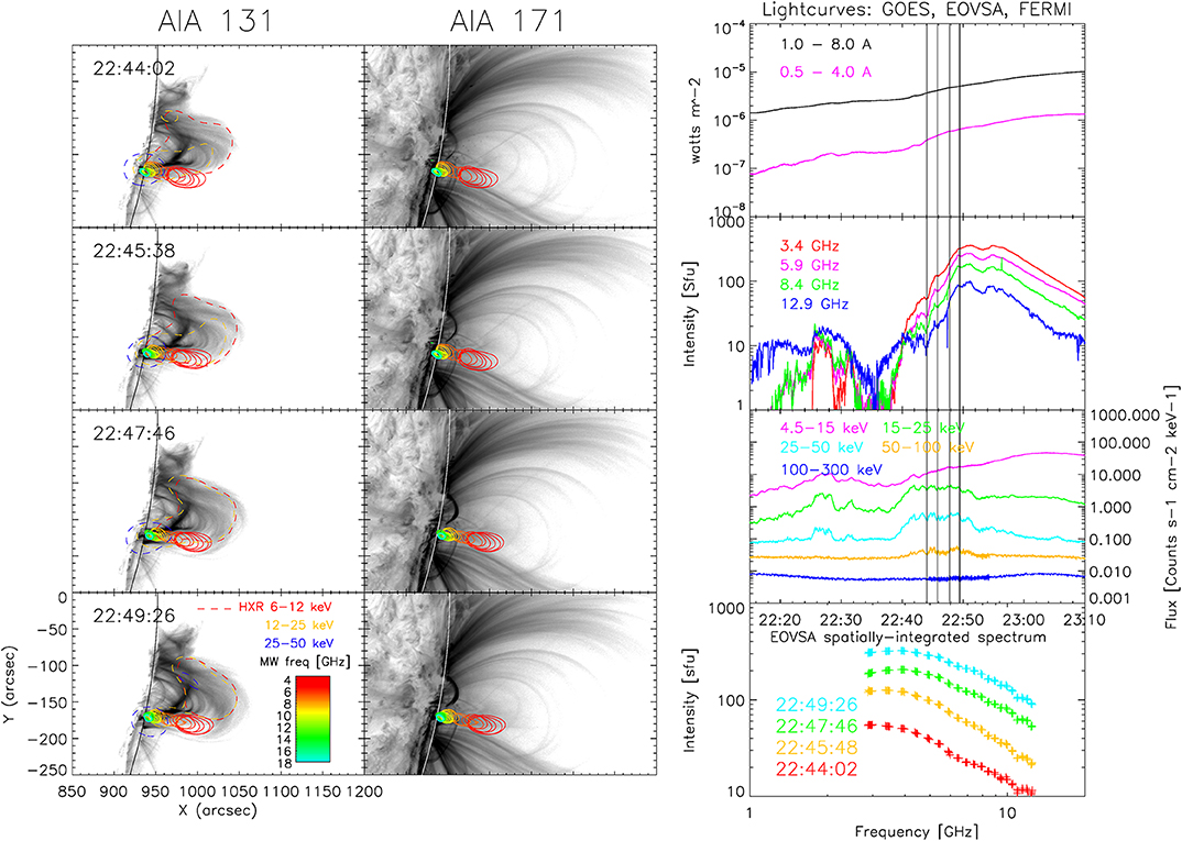
Figure 1. (Left) The flare development seen in MWs by EOVSA (solid contours [The color contours show 50% of the maximum intensity of each of 30 spw images]) and HXR from RHESSI (dashed contours), plotted on EUV 131 Å and 171 Å (background inverted grayscale) from SDO/AIA, at times t1–t4 (22:44:02–22:49:26 UT), indicated by four black vertical lines on the right panel. (Right), from the top: The soft X-ray, MW, and HXR lightcurves from GOES, EOVSA, and FERMI, respectively, and the total flux density spectra from EOVSA at four times images on the left panel (movie available). All contours are at 50% of the maximum intensity of each image.
The flare development throughout the time period shows that the MW high-frequency sources are co-spatial with the HXR non-thermal source (i.e., 25–50 keV) as often observed, indicating the presence of non-thermal electrons in the low solar atmosphere. The centroid of the 25–50 keV HXR source appears to lie very close to the west limb (c.f, Figure 1, blue dashed contours), which coincides with the central location of the AR at the photospheric level (S09W88). Although the coarse angular resolution of the detectors we use for imaging does not allow us to derive an accurate height of the HXR source above the limb as in, e.g., Krucker et al. (2015), we assume that it is likely a footpoint source located at chromospheric heights. At progressively lower frequencies, the MW sources extend higher in the corona, indicative of non-thermal electrons extending to higher heights where the magnetic field is relatively low, which is in line with earlier observations (Fleishman et al., 2017, 2018a,b).
Figure 2 overlays the EOVSA source contours with the 17 GHz image (inverted grayscale) obtained with Nobeyama RadioHeliograph (NoRH; Nakajima et al., 1994) near the end of the time period, for the same field of view as in Figure 1. A similar observation of an extended non-thermal electron population seen in low-frequency MWs was reported by Gary et al. (2018) in the X8.2 flare, which was produced 1 day later from the same AR. It is interesting to note, however, that the northern footpoint source faintly seen in NoRH image does not appear in the EOVSA images. This is most likely due to the different dynamic ranges of the two instruments. NoRH has 84 antennas, while EOVSA has only 13; thus, NoRH has better UV coverage, which results in a better dynamic range (although at lower spatial resolution). As a check, we confirmed that the northern MW source can be faintly seen when a wider, multi-band frequency-synthesis is used for EOVSA imaging, which increases the UV coverage at the expense of frequency resolution. This suggests that the EOVSA images correspond to the more strongly emitting leg of a large, asymmetric loop.
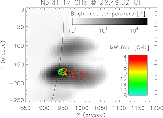
Figure 2. The EOVSA sources overlaid on the NoRH 17 GHz image (inverted grayscale) taken near the end of our time of interest, 22:49:26. The field of view is the same as in Figure 1. EOVSA's low frequency coverage reveals the large spatial extent of the non-thermal electron population in the corona with respect to height. At the same time, the higher dynamic range of the NoRH image at a single frequency reveals a possible asymmetry in the magnetic field strength of the loop containing these electrons.
The HXR low-energy sources (i.e., 6–12 and 12–25 keV) grow over time, very closely following the EUV 131 Å loops (Figure 1). We are likely observing a super-hot thermal loop of a few tens of MK, caused either by chromospheric evaporation after the initial particle acceleration seen in the HXR lightcurve, or direct heating from reconnection (Ning et al., 2018). The centroids of the EOVSA MW sources are slightly south of the southern leg of this thermal loop, which is a persistent feature (see Supplemental Movie 1). Therefore, the loop with the MW-emitting electrons appears to be slightly larger and possibly extends above the super-hot thermal loop. This combination of the HXR and MW source morphology fits the standard flare model: non-thermal electrons are injected from the acceleration region above the super-hot thermal loop, and then travel downward in the magnetic flux tube to emit GS radiation in the corona and bremsstrahlung in the chromosphere.
Both HXR and MW emissions are natural outcomes of non-thermal electrons accelerated in flares (White et al., 2011, and references therein). Observables of these emissions depend on both the non-thermal electron population and local properties of the flaring plasma in regions where those emissions are formed. As a result of the topological diversity of flares, the HXR and MW emissions display a variety of appearances and relationships. In some flares, both emissions are produced by a single population of non-thermal electrons in a single flaring loop (e.g., Fleishman et al., 2016b). In other cases, there could be different populations of the non-thermal electrons in distinct flaring loops, thus, different populations can dominate HXR and MW emissions. As a result, the non-thermal electron populations forming the two emissions can appear different in terms of spatial and/or energy distributions (Dennis, 1988; Kundu et al., 1994; Silva et al., 2000), even though they may have originated from the same acceleration site/process.
In this flare, the temporal correlation between HXR and MW lightcurves (seen in Figure 1 right panel) suggests a common origin of accelerated electrons responsible for the two emissions. Spatial relationships are consistent with the standard flare model, as explained in the previous section. Even so, the HXR- and MW-emitting energy ranges of the population may still exhibit dissimilar energy distributions and evolution thereof. Here, we focus on a comparison of the energy distributions of the non-thermal electrons derived from the spatially resolved MW and HXR data.
The MW emission in solar flares depends on many crucial physical parameters including magnetic field strength and orientation, non-thermal electron energy and angular distribution, and ambient plasma density and temperature. To derive those physical parameters, the spatially-resolved spectrum from each pixel in the high-resolution EOVSA images has to be forward-fit with the appropriate cost function. A suitable cost function (Gary et al., 2013; Fleishman et al., 2020) employs a numerical fast GS code that accounts for GS and free–free radio emission and absorption (Fleishman and Kuznetsov, 2010), since analytical approximations (Dulk and Marsh, 1982; Dulk, 1985) are too limited and too approximate for a meaningful forward fit. This fast GS code is an enhancement of a less accurate numerical Petrosian–Klein (PK) approximation of the exact GS equations (Melrose, 1968; Ramaty, 1969), which are highly complicated and computationally slow for our purposes. The fast GS code reduces computation time for GS emission by many orders of magnitude compared to exact calculations, while preserving the needed accuracy. Performing this model fitting, one can obtain the model fitting parameters over the entire source region at the observational cadence (Fleishman et al., 2020) in the form of evolving maps of the physical parameters. These parameter maps reveal the spatial distribution and the temporal evolution of the magnetic field and the plasma in the corona.
For the model spectral fitting, we adopt a homogeneous source along the line-of-sight (LOS) and fix the following parameters: plasma temperature, 30 MK; source depth, 5.8 Mm (equivalent to 8 arcsec); an isotropic pitch-angle distribution, and a single power-law electron energy distribution of the form
where A0 is the normalization factor, δ is the spectral index, n is the number density of the non-thermal electrons with energies between Emin and Emax, Emin is the minimum cutoff energy fixed at 17 keV, and Emax is the maximum cutoff energy fixed at 5 MeV. The initial values of the five free parameters are: non-thermal density, 107 cm−3; magnetic field strength, 400 G; viewing angle (angle between LOS and the magnetic field line), 60 degrees; thermal density, 1010 cm−3; and δ, 4.5. Although the currently available spectral fitting tool, GSFIT, accepts the T and Emax as free parameters, we found that they are not constrained for this flare; thus, they were fixed as described above.
The errors of the individual data points, needed to compute the χ2 metrics, were determined as follows. In each map we selected a region away from the microwave source and computed the rms value of the fluctuations. Then, to take into account the uncertainty introduced by a frequency-dependent spatial resolution of the EOVSA instrument, we added a frequency-dependent systematic uncertainty (Gary et al., 2013; Fleishman et al., 2020). The actual scatter of the adjacent spectral data points is noticeably smaller than the associated error bars (see examples in Figure A1 and Figure 5), which implies that the observational errors have been overestimated. For this reason, in what follows we will use a conservative χ2 upper threshold smaller than conventional values about one.
Figures 3, 4 show that the derived physical parameters vary smoothly in both space and time. Figure 3 shows a subset of the parameter maps (Supplemental Movie 2) at four selected times indicated in Figure 1 for: (a) magnetic field strength, (b) thermal electron density, (c) non-thermal electron density, (d) electron energy spectral index, (e) viewing angle, and (f) χ2 values of the fittings. The black contours are the 50% level of the radio maps at all 30 spws, while the red circles indicate the 50% contours of the 3.4 GHz images (spw 1) at each time. Visual inspection of individual fits suggests that the spectral fits with χ2 ≲ 0.1 are acceptable. Others may not be well fit because of: (1) a complex spectrum inconsistent with the uniform source model and contamination of the spectrum due to a sidelobe (see Figures A1A,B,E). These ill-fit spectra are excluded from the quantitative analysis. The χ2 values exceed the threshold in the lower-height part of the sources, which restricts our study to the coronal portion of the flaring loop.
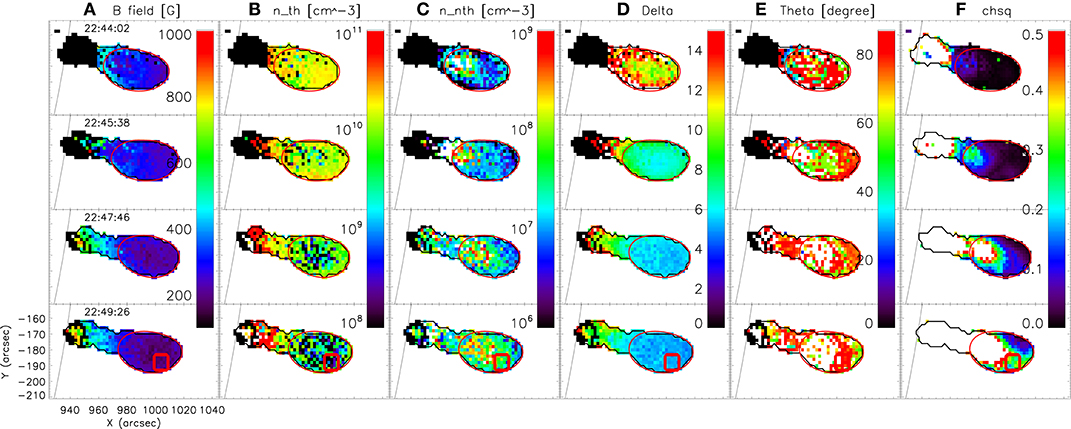
Figure 3. Snapshots of the coronal magnetic field and plasma parameter movie created by forward-fitting the spatially-resolved spectra of EOVSA images at every 4 s (movie available). The four times are the same times as shown in Figure 1, and the parameters are: (A) magnetic field strength, (B) thermal electron density, (C) non-thermal electron density, (D) electron energy spectral index, (E) viewing angle, and (F) χ2 values of the fittings. The black outline marks the union of the 50% contours of the original images at all 30 spws at each time, and the red circles indicate the 50% contours of the lowest frequency images (spw 1, 3.4 GHz) at each time. The time profiles of the parameters in the small red box are shown in Figure 4.
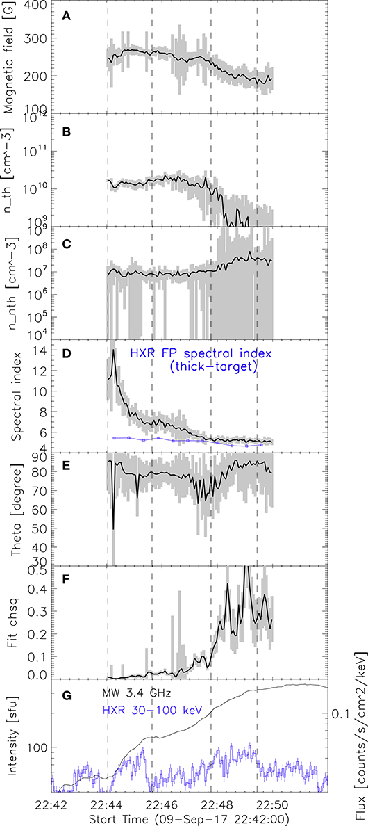
Figure 4. (A–F) Time profiles of the parameters from 25 pixels within the small red square marked in Figure 4: gray shade indicates the error bar of each parameter at each instance calculated as the standard deviation of the parameters over 25 pixels, black for their median. The spectral index inferred from the HXR analysis, interpreted as the index of electrons emitting in the lower atmosphere in section 3.2, is plotted in blue in (D). (G) The lowest-frequency MW lightcurve and the high-energy HXR lightcurve from RHESSI for reference, plotted on the same log scale. The dashed lines indicate time t1–t4.
In order to investigate evolution of the parameters, we selected a small area, marked by a red box in the bottom row of Figure 3, within the 3.4 GHz source that collectively showed χ2 values less than 0.1 for the longest time. The χ2 values in the area northward of the red box are lower, but many spectra have fewer or no optically-thick data points, making the fit formally better there but the parameters less reliable than in the red box.
Figure 4 shows evolution of the fit parameters in the red box. The black lines indicate the median values of the parameters from all 25 individual pixels, while the gray shade shows the associated error range calculated as the standard deviation of the parameters over these 25 pixels. In panel (g), we plot the lightcurves of MW 3.4 GHz and HXR 30–100 keV for the reference. The vertical dashed lines correspond to the times t1–t4 shown in Figures 1, 3. During the time range t1–t3, when χ2≲0.1, we see the following trends:
(1) magnetic field strength is about ~250 G; it does not show significant variations;
(2) thermal electron density varies within ~ (1−2) × 1010 cm−3,
(3) non-thermal electron density (above 17 keV) stays relatively constant, at ~107 cm−3,
(4) electron energy spectral index hardens significantly, from 14.1 ± 0.7 to 5.4 ± 0.1,
(5) viewing angle is in the range of 70 to 90 degrees.
To check if these parameter trends are reasonable, we inspect the MW spectral evolution at the center pixel of the red box up to time t3, as shown in Figure 5. The flux density of this spatially-resolved spectrum increases by about a factor of 10 in the peak, and more in optically-thin regions as the spectral slope decreases. This is the expected behavior when the magnetic field strength and non-thermal electron density are both constant, while the spectral index hardens (see Supplemental Movie 2 in Fleishman et al., 2020).
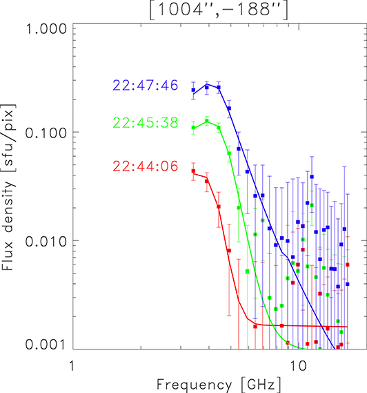
Figure 5. An example of the temporal evolution of the spectra and their fits, taken at one pixel inside the red box in Figure 3. The three times correspond to times t1–t3.
The trends (1) and (3) found above supports our initial view of the nature of the MW sources observed during this time period, that they are produced by the electrons accelerated at the acceleration cite and are transported inside the magnetic flux tube. This is in contrast with the result found by Fleishman et al. (2020), where they found the correlated decrease in magnetic field strength and increase in non-thermal electron density in the flare particle acceleration region.
In order to evaluate the effect of fixing a subset of parameters on the spectral fitting results, we perform a separate set of model fitting on the time series of spectra from the central pixel of the red square. First, we tested the effect of setting plasma temperature as a free parameter (initial temperature, 5 MK). We found as expected that the fit temperature values are unstable, varying from ~1 to ~25 MK, but are smaller than their error values, which means that plasma temperature cannot be well-constrained with these data. Even so, we found that the trends in other parameters in Figure 4 do not change significantly. We then doubled the source depth to 11.6 Mm (cf. 5.8 Mm) and found the derived magnetic field strength drops slightly to ~225 G without significant temporal variation, which is statistically consistent with 250 G reported above. We then ran the spectral fitting for two alternative values of Emin, 10 and 30 keV. For the former, we found that the magnetic field strength decreased with time from ~250 to ~210 G, while the non-thermal density remained stable at ~5 × 108 cm−3. For the latter, the magnetic field remained stable at ~200 G and the non-thermal density did not change from ~107 cm−3. Other fit parameters—thermal electron density, electron energy spectral index, and viewing angle—remained unaffected by changes in those fixed parameters.
One more possible limitation of our model spectral fitting is the assumed isotropic angular distribution of the non-thermal electrons. Although the GS emission certainly depends on the pitch-angle anisotropy (Fleishman and Melnikov, 2003), it is difficult to constrain without imaging spectro-polarimetry data, which is not yet available. Thus, at present we cannot firmly quantify possible bias introduced by the assumption of the isotropic angular distribution.
We conducted the spectral analysis in HXR using the OSPEX package (Schwartz et al., 2002). The spectra were obtained from t1–t4 using collimator 3 (which has a good energy resolution and reasonable instrument response matrix), with an integration time of 32 s, an energy range 1–106 keV, and with 1/3-keV-wide energy bins. We then fit the spectrum using the thermal (“vth”), thick-target model (“thick2”), and pile-up correction (“pileup_mod”) functions2. The equation for the thick-target model is:
where Flux(ϵ) is the photon flux at photon energy ϵ, nth is the number density of the thermal plasma, AU is one astronomical unit, m is the electron mass, c is the speed of light, σ(ϵ, E) is the bremsstrahlung cross section from equation (4) of Haug (1997), v is the non-thermal electron speed, and F(E0) is the electron flux density distribution function (electrons cm−2 s−1 keV−1), which is returned in the fitting3. In order to make this analysis consistent with the MW analysis, we only considered a single power-law and fixed the low energy cutoff of the electron energy distribution to 17 keV. The fitting energy range was ~6 to ~70 keV.
In this flare, the instrument had its attenuator state at A0, which made our observation the most affected by the pulse pile-up effect. In order to correct for this effect with some consistency, we have fit each spectrum manually while monitoring that the emission measure from the thermal fit and the first parameter of pile-up correction function (“coefficient to increase or decrease probability of pileup for energies > cutoff”) both increase correspondingly as the low-energy count rates increase during this time period. A sample of the spectral fit results is shown in Figure 6. The thermal fit returns a plasma temperature of ~32 MK and an emission measure of ~2 × 1046cm−3, which translates to a density of high ~108cm−3, if we estimate the thermal source volume from Figure 1 by assuming a bicone with a diameter of ~50” and a height of ~50”π. This plasma density is about an order of magnitude lower than that obtained from MW spectral fitting. However, we note that the plasma density from MW spectral fitting may not be well-constrained, since the spectra at higher heights do not have many optically-thick data points in our frequency range. In fact, it is possible to fit those spectra with lower plasma density while all other parameters are nearly the same as before, if we allow the high-frequency plateau from the free-free emission to be lower than the data points (but still within the error bars). Therefore, it is possible that the plasma density from the MW spectral fitting is overestimated and thus, the actual values could be consistent with the lower, HXR-derived values.
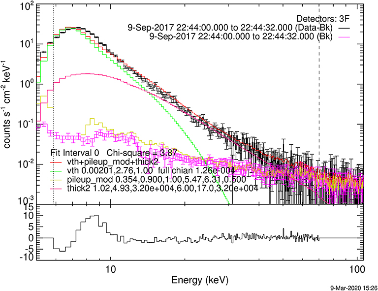
Figure 6. A example of the HXR spectral fit from OSPEX, at 22:44:16 UT.
We see in Figure 1 that the 25–50 keV sources obtained during this time period are most likely footpoint sources, and thus conclude that the fit parameters obtained from the thick-target function can be used to evaluate the powerlaw index of electrons producing the 25–50 keV emission. The time profile of this HXR-derived spectral index is plotted in Figure 4D as a blue line4.
It is apparent from Figure 4D that the δ values and their evolutions are very different in the corona and the thick-target source. However, we find that our coronal δ evolution from MW analysis seems to have some correspondence with the light curves of two emissions in Figure 4G. The interval up to t3 is divided into two episodes (guided by vertical dashed lines). In interval t1–t2, the HXR and MW lightcurves show rapid increase and the coronal δ also shows rapid hardening from 14.1 ± 0.7 to 6.8 ± 0.3. In interval t2–t3, the HXR and MW lightcurves show much slower increase (or perhaps none for HXR) and the coronal δ shows slower hardening as well, from 6.8 ± 0.3 to 5.4 ± 0.1. In the first episode, the HXR lightcurve's spiky shape suggests particle acceleration and the precipitation of the non-thermal electrons into the chromosphere. At the same time, the significant hardening of our coronal δ indicates a rapid increase in the number of high-energy non-thermal electrons in the corona, which is reflected by the rapid increase of the coronal MW emission at 3.4 GHz. This correspondence supports our initial view of this flare, where the particle acceleration occurs at or above the 3.4 GHz source, and the accelerated electrons travel downward along the magnetic field lines to emit GS radiation lower in the corona and thick-target bremsstrahung HXR radiation in the lower atmosphere.
In episode t2–t3 the HXR lightcurve suggests no significant increase in precipitation of non-thermal electrons to the chromosphere compared to the first episode. However, the coronal δ continues to harden. In order to comprehend this situation, we compare the observed evolution of the coronal electron energy spectrum with the model evolution provided by previous theoretical studies. We use the so-called trap-plus-precipitation (TPP) model (Melrose and Brown, 1976), which gives the analytical description of the evolution of the energy spectrum of the electrons in the magnetic trap under the influence of electron injection, energy losses due to Coulomb collisions, and precipitation out of the magnetic trap due to the pitch-angle diffusion by Coulomb interactions. This model considers the two extreme cases of (1) initial injection but no continuous injection and (2) no initial injection but continuous injection that is independent of time.
Let N(E, t) be the total number of electrons per unit energy range in the magnetic trap and Q(E, t) be the number of electron per unit energy injected into the trap in unit time. Assuming that the injection function is in the form of a single power-law with power-law index δ, the initial conditions for case (1) is
and for case (2),
where A and K are constants. The analytical solution of the transport equation for the temporal evolution of N(E, t) given by Melrose and Brown (1976) for case (1) is
For case (2),
where .
We take the electron energy spectrum observed in the corona at the end of the first episode as the spectrum of “initial injection” for case (1) and of “continuous injection” for case (2). Therefore, we use δ = 6.8 observed at 22:45:38 UT in Equations (3), (4). We also use cm−3 from the observation of thermal electron density shown in Figure 4. Lastly, we arbitrarily set A and K to be 1, and plot the normalized N(E, t) for two cases over several times during the time period of the second episode (128 s). Figure 7B shows the result for case (1), initial injection without continuous injection, and panel (c) shows the result for case (2), no initial injection but with continuous injection. Figure 7A shows the evolution of the total electron number spectrum derived from microwave data, obtained by multiplying the number density spectrum from Figures 4C,D by the total volume occupied by the small red square in Figure 3.
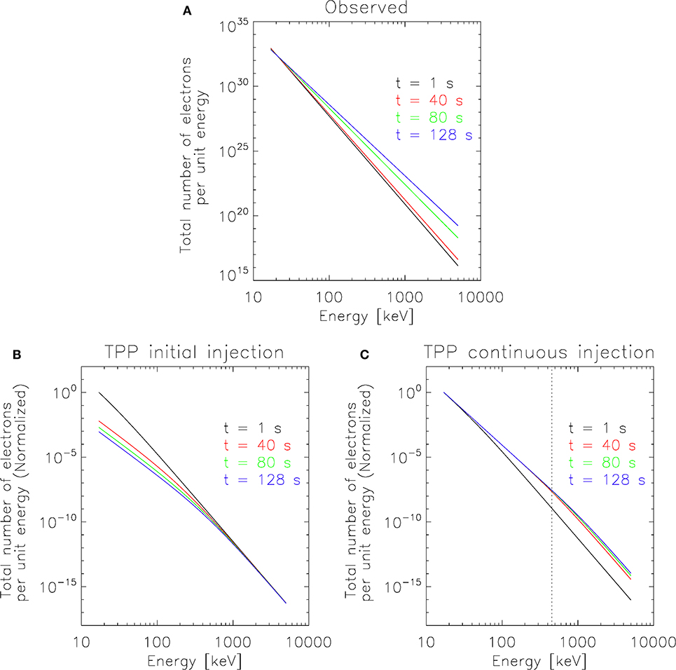
Figure 7. (A) The evolution of total electron number spectrum deduced from the MW fits, obtained by multiplying the number density spectrum from Figures 4C,D by the total volume occupied by the red box in Figure 3. (B,C) The modeled evolution of the total electron number spectrum (normalized) for the trap-plus-precipitation (TPP) model by Melrose and Brown (1976), over several times during the period of 22:45:38 to 22:47:46 UT, when the coronal δ from MW analysis shows a continued hardening despite a lack of apparent change in electron injection deduced from the HXR lightcurve. (B) Initial injection without continuous injection. (C) No initial injection but with continuous injection. The vertical dotted line marks the analytical value of the energy up to which the largest change in the low-energy spectral index is observed (see section 3.3).
It is clear from Figure 7 that the observed spectral evolution cannot be explained by the case with only initial injection, since the number of electrons in higher energies, up to several hundreds of keV, does not increase in the model. On the other hand, the increase in the number of those high-energy electrons is well-captured by the case with continuous injection, although the rate of increase seems to be faster in the model than in the observation. The result of the continuous injection model, as described in Melrose and Brown (1976), is that the spectrum evolves into a double-power law where the spectral index below the break energy Eb is harder than that above Eb by 1.5, and that the break energy increases with time as . If we calculate the evolution of δ in the model by assuming a single power-law with Emin = 17 keV and Emax as the energy up to which the largest change in δ is observed, which is with t = 128 s (~450 keV) and is marked by the vertical dashed line in Figure 7C, then the modeled coronal δ is 6.5 at t=1 s and 5.3 at t = 128 s. This is in agreement with our observed values of 6.8 ± 0.3 at time t2 and 5.4 ± 0.1 at time t3.
This result shows that the observed coronal δ hardening, which continued into the second episode, is broadly consistent with the TPP model of continuous electron injection into the coronal magnetic trap. However, the fact that there are still some differences, such as the rate of δ hardening and the values of δ above several hundred keV between the model and the observation, suggests that our observation cannot be fully explained by this simple model either. The TPP model's assumption of the time-independent power-law injection function is probably too simplistic, and the real injection function is most likely time-dependent and/or more complex than a single power-law. For example, it can be a double power-law, or a single power-law with the high-energy cut-off increasing in time due to a sustained acceleration process.
Let us discuss further the fact that there is a significant difference between coronal δ evolution from MW analysis and chromospheric δ evolution from HXR analysis. Compared to the coronal δ evolution of 14.1 ± 0.7 to 5.4 ± 0.1, the chromospheric δ changes from 5.4 ± 0.1 to 5.0 ± 0.1. We try to reconcile this observation to our initial picture where the same population of non-thermal electrons, accelerated in the same acceleration episode, is injected into the loop to produce all of the observed MW and HXR emission in this flare. One way to explain the different δ evolution in HXRs and MWs is if by assuming that the injected electrons have a double power-law energy spectrum and that our observed low-frequency coronal MW emission is more sensitive to the spectrum above a certain break energy Ebk (≠Eb). This double power-law spectrum could have a low-energy spectral index comparable to the observed HXR-derived δ up to Ebk and a much softer high-energy spectral index (or, a cut-off) above Ebk. The greater hardening of the MW-derived δ can then be reconciled by a hardening of the spectrum of the injected electrons only above Ebk, or by a sustained increase in time of Ebk itself. This would be in line with the recent study of Wu et al. (2019), which conducted the detailed simulation of the GS emission from the electrons with double power-law energy distribution and found that the increased high-energy electrons specified by the second spectral index result in a harder spectral index in the MW flux density spectrum,even if the total number of electrons does not change significantly.
In the previous section, we introduced the general picture of the evolution of the energy spectrum of the non-thermal electrons injected into the flaring loop in this flare. We did so by interpreting the temporal behavior of the parameters in a small representative volume in the context of the existing theory of electron transport in the corona. We now explore the collective behavior of the non-thermal electrons evolving in the flaring loop. Specifically, we calculate the total energy of non-thermal electrons contained in the corona, defined by the 50% contour of 3.4 GHz image (red contour in Figure 3), and plot this energy against time, to obtain the evolution of the total non-thermal electron energy contained in the corona. To do so, for each time frame we proceed with the following steps:
(1) Exclude all ill-fitted pixels within the 50% contour of the 3.4 GHz source,
(2) Calculate the non-thermal electron energy density in all well-fit pixels,
(3) Calculate the weighted mean of (2), then
(4) Multiply this weighted mean of the energy density by the total volume within the 50% contour of the 3.4 GHz source assuming a depth 5.8 Mm.
In step (1), we identify a pixel as ill-fitted if (1) the magnetic field solution is hitting its predefined upper limit of 3,000 G, (2) the number density solution is hitting its predefined lower limit of 103 cm−3, (3) the spectral index solution is hitting its predefined lower limit of 4 or upper limit of 15, or (4) χ2 > 0.1. Figure 6C shows the percentage of the well-fit pixels selected for the analysis with respect to the total number of pixels within 50% contour of 3.4 GHz source.
In step (2), we calculate the total energy contained in the coronal MW 3.4 GHz source, which we proposed in the previous section to be sensitive to the electrons that have energies higher than a certain Ebk. Therefore, we intentionally “cut” the observed energy distribution at Ebk. and obtain the energy density only above Ebk by using
where nE>Emin is n, the number density we obtained in section 3.1 (same as Equation 1), Emin is 17 keV, which was used in obtaining n, and α is the factor by which a certain Ebk is larger than 17 keV. We do not know the exact value of Ebk, but we adopt 70 keV for this analysis, since this is the upper limit of the fitting energy range for HXR spectral analysis that shows generally unchanged spectral indices over time.
In step (3), the weighted mean of the energy density is calculated by
where wε, i is the weight of energy density for ith well-fit pixel, calculated by where εerr, i is the error in energy density.
Finally, in step (4) we calculate the total volume within the 50% contour of the 3.4 GHz source by multiplying the total number of pixels within that contour by the 4 arcsec2 pixel area and the source depth of 5.8 Mm, as adopted in section 3.1. The evolution of this volume is plotted in Figure 8B.
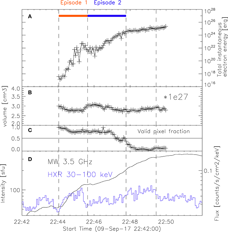
Figure 8. Evolution of parameters within the 50% contour of the observed MW 3.4 GHz source (red contours in Figure 3). (A) The total instantaneous energy of the non-thermal electrons with energies >70 keV. (B) The total volume. (C) The percentage of the total number of pixels in the source that are well-fit and hence selected for analysis. (D) The same lightcurves from Figure 4G for reference. The dashed lines mark times t1–t4.
Figure 8A shows the evolution of the total instantaneous energy of the non-thermal electrons having energies >70 keV contained within the 50% contour of the observed MW 3.4 GHz sources. Figure 8D shows, for reference, the lightcurves from Figure 4G, and the four vertical dashed lines mark the same time boundaries as in Figures 1, 3, 4. Figure 8A shows that, overall, there is a significant increase in the total instantaneous energy of electrons >70 keV contained in the coronal source. The energies corresponding to each time boundary are 3.8 ± 0.5 × 10¹⁷ erg at t1, 4.9 ± 0.8 × 10²¹ erg at t2, 3.9 ± 0.2 × 1024 erg at t3, and 7.6 ± 0.5 × 1024 erg at t4. We note that the fraction of well-fit pixels within the source significantly decreases after t3 (see Figure 8C), so the results after this time may not be as reliable as in the preceding time intervals. However, up to t3, at least half of the pixels within the 50% contour of 3.4 GHz sources are considered for the analysis, so our results can be taken with more confidence during this time. From Figure 8A it is observed that the total energy reaches about 1022 erg by time t2, and increases by ~3 orders of magnitude during episode t2–t3.
Although this analysis has been done assuming that the observed radio emission during our time of interest is produced by non-thermal electrons, it is possible that, at least during the time when the inferred spectral index is very soft (e.g., during episode 1), the emission is due to thermal electrons. In fact, most of the time during episode 1, we find that the observed spectra within the red box in Figure 4 could be reproduced without the need for a non-thermal electron distribution. Instead, they could be produced by gyrosynchrotron emission generated by electrons with a ~20 MK thermal distribution in a source with the same magnetic field, thermal electron density, and viewing angle. Therefore, the result in Figure 8A during episode t1–t2 should be taken as the extreme case of considering all MW-emitting electrons to be non-thermal. However, purely thermal emission is excluded for t2–t3, since many pixels start showing spectra that are too hard in their optically-thin sides to be explained by thermal gyrosynchrotron emission. Therefore, we believe that our results during t2–t3 truly reflect the rise in the energy of non-thermal electrons with energies >70 keV in the corona.
In this study, we analyzed the evolution of the non-thermal electrons accelerated during the impulsive phase of the M1.2 flare on 2017 September 9. We focused on a ~6-min period when a significant increase of MW emission was observed compared to the level of increase in HXR emission. We used multi-wavelength observations to evaluate the overall spatial distribution of electrons in the flare, and combined it with the total energy and energy distribution of electrons derived from the combination of MW and HXR analysis. In particular, our MW analysis was conducted using the new technique of numerical forward-fitting of spatially-resolved MW spectra derived from multi-frequency images from EOVSA. This enabled the quantitative calculation of the spatially-resolved evolution of the non-thermal electrons in the corona. The summary of the main results from this work is the following.
(1) The comparison of EUV-loops, the locations of low- and high-energy HXR emission sources, and the distribution of MW images from 3.4 to 18 GHz suggest that the spatial distribution of the non-thermal electrons in this flare generally fits the traditional standard flare model morphology. We infer that the electrons are accelerated in a region located above the hot loop visible in AIA 131 Å and RHESSI 6-12 keV images and are injected into a somewhat larger “non-thermal” flare loop connecting the low-frequency coronal MW sources with the co-spatial 20-50 keV HXR and 17 GHz MW sources in the lower atmosphere.
(2) The comparison of the spectral index of the non-thermal electrons derived from HXR and MW analysis reveals, however, that their values and evolution are significantly different. More specifically, the spectral index of the non-thermal electrons associated with the coronal 3.4 GHz MW source undergoes much faster hardening than that associated with the footpoint HXR source. The former hardens from 14.1 ± 0.7 to 5.4 ± 0.1 and the latter changes from 5.4 ± 0.1 to 5.0 ± 0.1 over the same period of 128 s. Because the energy range of electrons producing HXR and MW emission differ, we interpret this discrepancy as reflecting a different spectral evolution in different parts of the energy spectrum.
(3) Our findings vividly show that the high-energy tail of the non-thermal electron distribution, which is responsible for the MW emission, underwent more significant evolution compared with the low-energy counterpart of the distribution for this flare. In-depth analysis focusing on the spectral evolution of the coronal electron population suggests that there was a sustained acceleration and continued injection of non-thermal electrons in the corona even when there was no significant signature for that in the HXR lightcurve for a period of time. The difference in the spectral evolution is reconciled by adopting that the energy spectrum of this injected population has a double power-law or a break-down spectrum above an evolving (rising in time) break energy Ebk in the form of a cut-off. The population with energies higher than the break energy, to which the MW emission is more sensitive than the HXR emission, have undergone greater spectral hardening, perhaps, due to the sustained acceleration.
(4) Based on this picture of the evolution of the energy spectrum of the non-thermal electrons injected into the flaring loop, we estimated the evolution of the total instantaneous non-thermal (>70 keV) electron energy contained in a coronal volume enclosed by the coronal 3.4 GHz MW source. We find a significant increase of several orders of magnitude in the total energy of these electrons contained in the coronal source during the ~4 min period of interest of the flare impulsive phase.
An interesting observation, shown in Figure 8A, is that the total instantaneous non-thermal electron energy contained in the coronal source continues to increase during the period we studied. Under the assumption of a single loop, it is interesting to compare this evolution with the development of the total energy flux deposited by HXR-emitting non-thermal electrons into the lower atmosphere. We plot the evolution of the total energy flux of HXR-emitting electrons in Figure 9, using the result of the analysis from section 3.2. We use the modification of Equation (7), , where is the total electron flux obtained from the thick-target spectral fit. Although this cannot be directly compared with Figure 8A because of the different units, this clearly indicates that the evolution of the total energy of non-thermal electrons in the lower atmosphere is different from that in the corona.
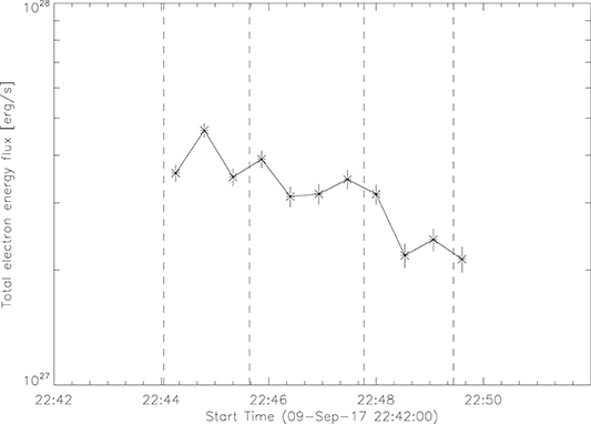
Figure 9. The evolution of the total energy flux of HXR-emitting electrons in the chromosphere, using the result of the analysis from section 3.2.
A consistency check of the single-population scenario can be performed by assuming a single power-law distribution that extends from tens of keV to hundreds of keV, covering both HXR-emitting and MW-emitting population of energetic electrons, at the time when the spectral indices from two analysis match, around t3 (see Figure 4D). In this analysis we use a simple relation where is the non-thermal electron flux distribution from HXR analysis, n(E) is the non-thermal electron density distribution from MW analysis, is the mean speed of non-thermal electrons, and A is the area of the thick-target HXR emission. We obtain from OSPEX analysis that electrons/s, estimate A from the 50% contour of 18 GHz MW image in Figure 1 left panels (circular area with ~10″ diameter), and from the energy distribution. This yields n ~ 3 × 107 cm−3, which roughly agrees with the value of n ~ 107 cm−3 we obtained from MW analysis at this time.
An alternative explanation for the difference in δ development is that we are observing two electron populations belonging to different loop systems. For instance, our HXR-producing population may be reflecting the evolution of the non-thermal electrons in a small loop unresolved by RHESSI. This will allow the δ evolution in the corona and lower atmosphere to be unrelated, as in our observation. In fact, Kuroda et al. (2018) revealed the presence of an extended “HXR-invisible” non-thermal electron population outside of the traditional flare geometry at one time during another flare by using the RHESSI and the EOVSA data, and this snap-shot model required two separate loops to simultaneously reproduce the observed low-frequency MW emission and HXR/high-frequency MW emission. If we adopt a two-loop scenario for this study, however, the two loops must be dynamically connected since time profiles of low-frequency MWs at higher heights are very well-correlated with higher-frequency MWs co-spatial with the 25-50 keV HXR source.
Lastly, we note that electron pitch-angle anisotropy may change our result in Figure 4 and possibly affect our conclusions. Differences in the inverted non-thermal electron energy distribution for isotropic vs. anisotropic (e.g., beam-like) distributions have been reported in MW both observationally (Lee and Gary, 2000; Melnikov et al., 2002; Altyntsev et al., 2008) and in simulations (Fleishman and Kuznetsov, 2010). For HXR, the bremsstrahlung cross section is also pitch-angle dependent (Equation 2 BN in Koch and Motz 1959). Therefore, an anisotropic electron distribution would produce a HXR photon spectrum that deviates from our results which assume an isotropic electron distribution (see, e.g., discussions in Massone et al., 2004; Chen and Bastian, 2012). However, exploring the effects of different pitch-angle distributions is beyond the scope of this study.
Although the origin of the striking dissimilarities in the evolution of the spectral indices of the non-thermal electrons in the corona and the chromosphere are open to debate, it is important to note that these differences are only revealed through the spatially-resolved analysis of the evolving coronal MW sources below ~10 GHz. The continued electron injection and hardening revealed by the coronal MW analysis seems to affect only the highest electron energies, and therefore lacks the expected counterpart signature in the HXR source. Since the location of the MW peak frequency is most sensitive to the magnetic field strength of the source, this characteristic informs us about non-thermal electrons higher in the corona (weaker magnetic field), where the HXR analysis becomes increasingly difficult due to the scarcity of the target plasma for bremsstrahlung.
EOVSA data are freely available from http://ovsa.njit.edu/data-browsing.html. Fully processed EOVSA spectral imaging data in IDL save format can be downloaded from https://www.dropbox.com/s/6dk40smvea8f66f/eovsa_20170909T223518-231518_r2_XX.sav?dl=0. The package for microwave data fitting, GSFIT, is included in the publicly available library SolarSoftWare under the Packages category at http://www.lmsal.com/solarsoft/ssw_packages_info.html.
NK processed the raw data, performed the fitting, initial analysis of the results, and wrote the initial draft. GF developed the fitting methodology. DG led the construction and commissioning of the EOVSA, developed the strategy for taking and calibrating the data for microwave spectroscopy. GN developed the GSFIT package used in the automated fitting. BC and SY developed the microwave spectral imaging and self-calibration strategy. All authors involved in the discussion and contributed to manuscript preparation.
EOVSA operation is supported by NSF grant AST-1910354. NK was partially supported by the NASA Living With a Star Jack Eddy Postdoctoral Fellowship Program, administered by UCAR's Cooperative Programs for the Advancement of Earth System Science (CPAESS) under award #NNX16AK22G. GF, DG, GN, BC, and SY are supported by NSF grants AGS-1654382, AST-1910354, AGS-1817277, AGS-1743321, and NASA grants 80NSSC18K0667, NNX17AB82G, 80NSSC18K1128, and 80NSSC19K0068 to New Jersey Institute of Technology.
The authors declare that the research was conducted in the absence of any commercial or financial relationships that could be construed as a potential conflict of interest.
The authors thank the scientists and engineers who helped design and build EOVSA, especially Gordon Hurford, Stephen White, James McTiernan, Wes Grammer, Kjell Nelin, and Tim Bastian.
The Supplementary Material for this article can be found online at: https://www.frontiersin.org/articles/10.3389/fspas.2020.00022/full#supplementary-material
Supplemental Movie 1. The movie corresponding to Figure 1 is available as a supplemental material fig1_movie.avi.
Supplemental Movie 2. The movie corresponding to Figure 3 is available as a supplemental material fig3_movie.avi.
1. ^http://sprg.ssl.berkeley.edu/~tohban/browser/
2. ^See documentation at: https://hesperia.gsfc.nasa.gov/ssw/packages/spex/idl/object_spex/fit_model_components.txt.
3. ^See documentation at: https://hesperia.gsfc.nasa.gov/ssw/packages/xray/doc/brm_thick_doc.pdf.
4. ^Since the spectral index returned by OSPEX fit is that of the electron flux density spectrum, we add 0.5 to the OSPEX values in order to make them comparable to our MW-derived δ, which is that of a number density spectrum. i.e., n(E) = F(E)/v, where , , and v ∝ E1/2.
Altyntsev, A. T., Fleishman, G. D., Huang, G. L., and Melnikov, V. F. (2008). A broadband microwave burst produced by electron beams. Astrophys. J. 677, 1367–1377. doi: 10.1086/528841
Aschwanden, M. J., Holman, G., O'Flannagain, A., Caspi, A., McTiernan, J. M., and Kontar, E. P. (2016). Global energetics of solar flares. III. Nonthermal energies. Astrophys. J. 832:27. doi: 10.3847/0004-637X/832/1/27
Atwood, W. B., Abdo, A. A., Ackermann, M., Althouse, W., Anderson, B., Axelsson, M., et al. (2009). The large area telescope on the Fermi gamma-ray space telescope mission. Astrophys. J. 697, 1071–1102. doi: 10.1088/0004-637X/697/2/1071
Chen, B., and Bastian, T. S. (2012). The role of inverse compton scattering in solar coronal hard x-ray and γ-ray sources. Astrophys. J. 750:35. doi: 10.1088/0004-637X/750/1/35
Dennis, B. R. (1988). Solar flare hard x-ray observations. Solar Phys. 118, 49–94. doi: 10.1007/BF00148588
Dulk, G. A. (1985). Radio emission from the sun and stars. Annu. Rev. Astron. Astrophys. 23, 169–224. doi: 10.1146/annurev.aa.23.090185.001125
Dulk, G. A., and Marsh, K. A. (1982). Simplified expressions for the gyrosynchrotron radiation from mildly relativistic, nonthermal and thermal electrons. Astrophys. J. 259, 350–358. doi: 10.1086/160171
Emslie, A. G., Dennis, B. R., Shih, A. Y., Chamberlin, P. C., Mewaldt, R. A., Moore, C. S., et al. (2012). Global energetics of thirty-eight large solar eruptive events. Astrophys. J. 759:71. doi: 10.1088/0004-637X/759/1/71
Fleishman, G. D., Gary, D. E., Chen, B., Kuroda, N., Yu, S., and Nita, G. M. (2020). Decay of the coronal magnetic field can release sufficient energy to power a solar flare. Science 367, 278–280. doi: 10.1126/science.aax6874
Fleishman, G. D., Kontar, E. P., Nita, G. M., and Gary, D. E. (2011). A cold, tenuous solar flare: acceleration without heating. Astrophys. J. Lett. 731:L19. doi: 10.1088/2041-8205/731/1/L19
Fleishman, G. D., Kontar, E. P., Nita, G. M., and Gary, D. E. (2013). Probing dynamics of electron acceleration with radio and x-ray spectroscopy, imaging, and timing in the 2002 April 11 solar flare. Astrophys. J. 768:190. doi: 10.1088/0004-637X/768/2/190
Fleishman, G. D., and Kuznetsov, A. A. (2010). Fast gyrosynchrotron codes. Astrophys. J. 721, 1127–1141. doi: 10.1088/0004-637X/721/2/1127
Fleishman, G. D., Loukitcheva, M. A., Kopnina, V. Y., Nita, G. M., and Gary, D. E. (2018a). The coronal volume of energetic particles in solar flares as revealed by microwave imaging. Astrophys. J. 867:81. doi: 10.3847/1538-4357/aae0f6
Fleishman, G. D., and Melnikov, V. F. (2003). Gyrosynchrotron emission from anisotropic electron distributions. Astrophys. J. 587, 823–835. doi: 10.1086/368252
Fleishman, G. D., Nita, G. M., and Gary, D. E. (2009). Dynamic magnetography of solar flaring loops. Astrophys. J. Lett. 698, L183–L187. doi: 10.1088/0004-637X/698/2/L183
Fleishman, G. D., Nita, G. M., and Gary, D. E. (2017). A large-scale Plume in an X-class solar flare. Astrophys. J. 845:135. doi: 10.3847/1538-4357/aa81d4
Fleishman, G. D., Nita, G. M., Kontar, E. P., and Gary, D. E. (2016a). Narrowband gyrosynchrotron bursts: probing electron acceleration in solar flares. Astrophys. J. 826:38. doi: 10.3847/0004-637X/826/1/38
Fleishman, G. D., Nita, G. M., Kuroda, N., Jia, S., Tong, K., Wen, R. R., et al. (2018b). Revealing the evolution of non-thermal electrons in solar flares using 3D modeling. Astrophys. J. 859:17. doi: 10.3847/1538-4357/aabae9
Fleishman, G. D., Xu, Y., Nita, G. N., and Gary, D. E. (2016b). Validation of the coronal thick target source model. Astrophys. J. 816:62. doi: 10.3847/0004-637X/816/2/62
Gary, D. E., Chen, B., Dennis, B. R., Fleishman, G. D., Hurford, G. J., Krucker, S., et al. (2018). Microwave and hard x-ray observations of the 2017 September 10 solar limb flare. Astrophys. J. 863:83. doi: 10.3847/1538-4357/aad0ef
Gary, D. E., Fleishman, G. D., and Nita, G. M. (2013). Magnetography of solar flaring loops with microwave imaging spectropolarimetry. Solar Phys. 288, 549–565. doi: 10.1007/s11207-013-0299-3
Glesener, L., and Fleishman, G. D. (2018). Electron acceleration and jet-facilitated escape in an M-class solar flare on 2002 August 19. Astrophys. J. 867:84. doi: 10.3847/1538-4357/aacefe
Haug, E. (1997). On the use of nonrelativistic bremsstrahlung cross sections in astrophysics. Astron. Astrophys. 326, 417–418.
Hoyng, P., Duijveman, A., Machado, M. E., Rust, D. M., Svestka, Z., Boelee, A., et al. (1981). Origin and location of the hard x-ray emission in a two-ribbon flare. Astrophys. J. Lett. 246:L155. doi: 10.1086/183574
Koch, H. W., and Motz, J. W. (1959). Bremsstrahlung cross-section formulas and related data. Rev. Modern Phys. 31, 920–955. doi: 10.1103/RevModPhys.31.920
Krucker, S., and Battaglia, M. (2014). Particle densities within the acceleration region of a solar flare. Astrophys. J. 780:107. doi: 10.1088/0004-637X/780/1/107
Krucker, S., Hudson, H. S., Glesener, L., White, S. M., Masuda, S., Wuelser, J. P., et al. (2010). Measurements of the coronal acceleration region of a solar flare. Astrophys. J. 714, 1108–1119. doi: 10.1088/0004-637X/714/2/1108
Krucker, S., Saint-Hilaire, P., Hudson, H. S., Haberreiter, M., Martinez-Oliveros, J. C., Fivian, M. D., et al. (2015). Co-spatial white light and hard x-ray flare footpoints seen above the solar limb. Astrophys. J. 802:19. doi: 10.1088/0004-637X/802/1/19
Kundu, M. R., White, S. M., Gopalswamy, N., and Lim, J. (1994). Millimeter, microwave, hard x-ray, and soft x-ray observations of energetic electron populations in solar flares. Astrophys. J. Suppl. 90:599. doi: 10.1086/191881
Kuroda, N., Gary, D. E., Wang, H., Fleishman, G. D., Nita, G. M., and Jing, J. (2018). Three-dimensional forward-fit modeling of the hard x-ray and microwave emissions of the 2015 June 22 M6.5 Flare. Astrophys. J. 852:32. doi: 10.3847/1538-4357/aa9d98
Lee, J., and Gary, D. E. (2000). Solar microwave bursts and injection pitch-angle distribution of flare electrons. Astrophys. J. 543, 457–471. doi: 10.1086/317080
Lemen, J. R., Title, A. M., Akin, D. J., Boerner, P. F., Chou, C., Drake, J. F., et al. (2012). The atmospheric imaging assembly (AIA) on the solar dynamics observatory (SDO). Solar Phys. 275, 17–40. doi: 10.1007/s11207-011-9776-8
Lin, R. P., Dennis, B. R., Hurford, G. J., Smith, D. M., Zehnder, A., Harvey, P. R., et al. (2002). The Reuven Ramaty high-energy solar spectroscopic imager (RHESSI). Solar Phys. 210, 3–32. doi: 10.1023/A:1022428818870
Lin, R. P., and Hudson, H. S. (1971). 10 100 keV electron acceleration and emission from solar flares. Solar Phys. 17, 412–435. doi: 10.1007/BF00150045
Massone, A. M., Emslie, A. G., Kontar, E. P., Piana, M., Prato, M., and Brown, J. C. (2004). Anisotropic bremsstrahlung emission and the form of regularized electron flux spectra in solar flares. Astrophys. J. 613, 1233–1240. doi: 10.1086/423127
Masuda, S., Kosugi, T., Hara, H., Tsuneta, S., and Ogawara, Y. (1994). A loop-top hard X-ray source in a compact solar flare as evidence for magnetic reconnection. Nature 371, 495–497. doi: 10.1038/371495a0
Melnikov, V. F., Shibasaki, K., and Reznikova, V. E. (2002). Loop-top nonthermal microwave source in extended solar flaring loops. Astrophys. J. Lett. 580, L185–L188. doi: 10.1086/345587
Melrose, D. B. (1968). The emission and absorption of waves by charged particles in magnetized plasmas. Astrophys. Space Sci. 2, 171–235. doi: 10.1007/BF00651567
Melrose, D. B., and Brown, J. C. (1976). Precipitation in trap models for solar hard X-ray bursts. Mon. Not. R. Astron. Soc. 176, 15–30. doi: 10.1093/mnras/176.1.15
Nakajima, H., Nishio, M., Enome, S., Shibasaki, K., Takano, T., Hanaoka, Y., et al. (1994). The Nobeyama radioheliograph. IEEE Proc. 82, 705–713. doi: 10.1109/5.284737
Ning, H., Chen, Y., Wu, Z., Su, Y., Tian, H., Li, G., et al. (2018). Two-stage energy release process of a confined flare with double HXR peaks. Astrophys. J. 854:178. doi: 10.3847/1538-4357/aaaa69
Nita, G. M., Hickish, J., MacMahon, D., and Gary, D. E. (2016). EOVSA implementation of a spectral kurtosis correlator for transient detection and classification. J. Astron. Instrum. 5, 1641009–7366. doi: 10.1142/S2251171716410099
Nitta, N., and Kosugi, T. (1986). Energy of microwave-emitting electrons and hard x-ray / microwave source model in solar flares. Solar Phys. 105, 73–85. doi: 10.1007/BF00156378
Ramaty, R. (1969). Gyrosynchrotron emission and absorption in a magnetoactive plasma. Astrophys. J. 158:753. doi: 10.1086/150235
Schwartz, R. A., Csillaghy, A., Tolbert, A. K., Hurford, G. J., McTiernan, J., and Zarro, D. (2002). RHESSI data analysis software: rationale and methods. Solar Phys. 210, 165–191. doi: 10.1023/A:1022444531435
Silva, A. V. R., Wang, H., and Gary, D. E. (2000). Correlation of microwave and hard x-ray spectral parameters. Astrophys. J. 545, 1116–1123. doi: 10.1086/317822
White, S. M., Benz, A. O., Christe, S., Fárník, F., Kundu, M. R., Mann, G., et al. (2011). The relationship between solar radio and hard x-ray emission. Space Sci. Rev. 159, 225–261. doi: 10.1007/s11214-010-9708-1
Wu, Z., Chen, Y., Ning, H., Kong, X., and Lee, J. (2019). Gyrosynchrotron emission generated by nonthermal electrons with the energy spectra of a broken power law. Astrophys. J. 871:22. doi: 10.3847/1538-4357/aaf474
We show in here the sample of spatially-resolved MW spectra (black asterisks) and the fit results (green lines). The examples of successful fits are (C,D) and those of unsuccessful fits are (A,B,E). The pixel selected for (D,E) is one of the pixels in the small red box shown in Figure 3. (A–D) show the results from 22:46:14 UT, a time between t2 and t3, and Panel (E) shows the result from the same pixel as (D) but at t4, at the end of our fitting time period.
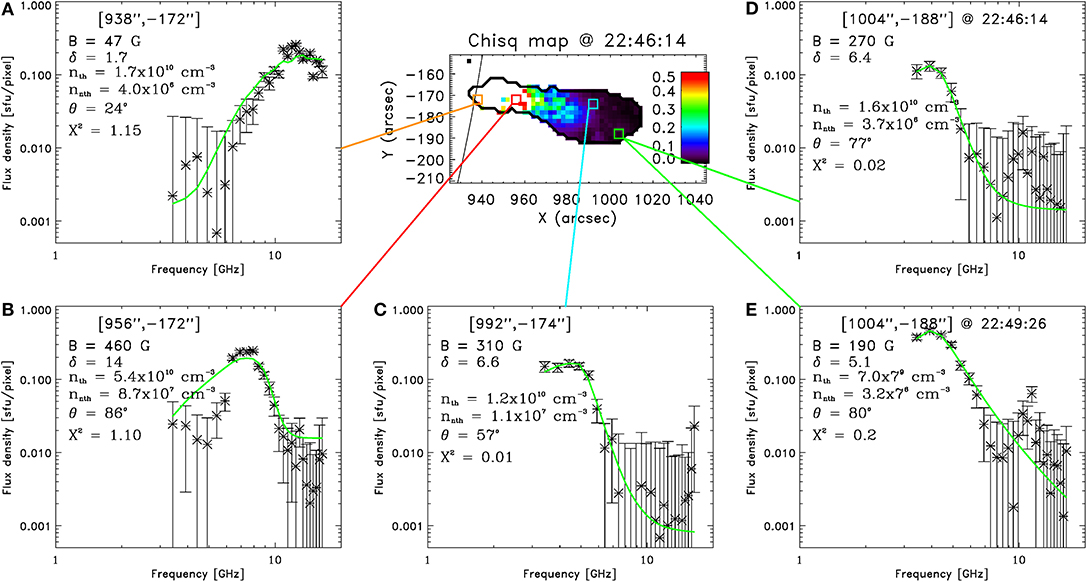
Figure A1. (A) An unsuccessful fit due to the high peak frequency leading to the shortage of good data points in the optically-thin frequency range. Note the unrealistically low magnetic field value of 47 G, far lower than fits of surrounding pixels. (B) An unsuccessful fit due to the unusually narrow peak shape of the observed spectrum. (C,D) Examples of successful fits. Note that the magnetic field strength reasonably decreases with height. The χ2 value is < 0:1, which is the criterion used in the quantitative analysis in Section 3. (E) An unsuccessful fit due to the contamination of the spectrum by a sidelobe of the highfrequency source at ~ 11 GHz. The result is shown from the same pixel as (D) but at later time, at 22:49:26. This type of unsuccessful fit was more prelavent toward the end of our fitting time period as the flare emission intensity increased. Note that with this fit, the spectral index may be reported harder than the actual value. The χ2 value is again > 0:1.
Keywords: solar flares, microwave, imaging spectroscopy, non-thermal electrons, numerical modeling, X-ray, corona, evolution
Citation: Kuroda N, Fleishman GD, Gary DE, Nita GM, Chen B and Yu S (2020) Evolution of Flare-Accelerated Electrons Quantified by Spatially Resolved Analysis. Front. Astron. Space Sci. 7:22. doi: 10.3389/fspas.2020.00022
Received: 05 January 2020; Accepted: 27 April 2020;
Published: 27 May 2020.
Edited by:
Xueshang Feng, National Space Science Center (CAS), ChinaReviewed by:
Yao Chen, Shandong University, ChinaCopyright © 2020 Kuroda, Fleishman, Gary, Nita, Chen and Yu. This is an open-access article distributed under the terms of the Creative Commons Attribution License (CC BY). The use, distribution or reproduction in other forums is permitted, provided the original author(s) and the copyright owner(s) are credited and that the original publication in this journal is cited, in accordance with accepted academic practice. No use, distribution or reproduction is permitted which does not comply with these terms.
*Correspondence: Natsuha Kuroda, bmt1cm9kYUB1Y2FyLmVkdQ==
Disclaimer: All claims expressed in this article are solely those of the authors and do not necessarily represent those of their affiliated organizations, or those of the publisher, the editors and the reviewers. Any product that may be evaluated in this article or claim that may be made by its manufacturer is not guaranteed or endorsed by the publisher.
Research integrity at Frontiers
Learn more about the work of our research integrity team to safeguard the quality of each article we publish.