Discovery of an Electron Gyroradius Scale Current Layer: Its Relevance to Magnetic Fusion Energy, Earth's Magnetosphere, and Sunspots

In the Earth's magnetosphere, sunspots and magnetic cusp fusion devices, the boundary between the plasma and the magnetic field is marked by a diamagnetic current layer with a rapid change in plasma pressure and magnetic field strength. First principles numerical simulations were conducted to investigate this boundary layer with a spatial resolution beyond electron gyroradius while incorporating a global equilibrium structure. The boundary layer thickness is discovered to be on the order of electron gyroradius scale due to a self-consistent electric field suppressing ion gyromotion at the boundary. Formed at the scale of the electron gyroradius, the electric field plays a critical role in determining equilibrium structure and plasma transport. The discovery highlights the necessity to incorporate electron gyroradius scale physics in studies aimed at advancing our understanding of fusion devices, the magnetosphere and sunspots.

Introduction

In many plasma systems, the plasma is surrounded by magnetic fields leading to a fascinating array of natural and manmade phenomena. Plasma jet formation from accretion disks, Earth's magnetosphere, sunspots, and magnetic fusion devices are examples of plasma interaction with magnetic fields. At the boundary between the plasma and the magnetic field, if there is a change in plasma pressure or magnetic field strength, gyromotions of electrons and ions generate current, known as diamagnetic current, separating the plasma, and magnetic field (Krall and Trivelpiece, 1973). Among examples of plasma diamagnetic effects are the magnetopause in the Earth's magnetosphere, sharp boundary layers in magnetic cusp fusion devices, and the dark patches of sunspots (Hale, 1908; Chapman and Ferraro, 1930; Berkowitz et al., 1958; Braginskii and Kadomtsev, 1959; Sonnerup and Cahill, 1967; Spalding, 1971; Borrero and Ichimoto, 2011). In these systems, a diamagnetic current layer marks the boundary across which plasma penetration or loss to the magnetic field region is greatly reduced. The diamagnetic effect in these systems has been studied extensively, leading to the development of magnetohydrodynamics (MHD), the standard model for many solar, astrophysics and fusion plasmas over the past 50 years (Alfvén, 1942; Cowling, 1957).

However, an ab initio solution of plasma diamagnetic effects had remained elusive with some of the most fundamental questions yet to be answered (Alfvén, 1963). For example, there has been no definitive answer to the thickness of the diamagnetic current layer. Also unknown are the respective contributions of ions and electrons to the plasma diamagnetic current since there is significant difference in their gyroradii, a factor of 43 in the case of hydrogen ions at the same temperature as electrons. The lack of understanding remains because we are still trying to understand plasma dynamics at the scale of the electron the gyroradius, the fundamental, yet smallest, length scale of plasma diamagnetism. While there have been many theoretical and numerical studies to investigate the boundary layer structure, these studies have been limited due to geometrical complexities and technical challenges and have been unable to resolve electron gyroradius scale physics while incorporating the global equilibrium structure (Dungey, 1961; Grad, 1961; Haines, 1977; Berchem, 1990; Bessho et al., 2016). At the same time, a number of observations indicate the importance of electron scale phenomena at the boundary such as formation of electron scale ion flow in laboratory magnetic cusp experiments (Hershkowitz et al., 1975). The recently launched Magnetospheric Multiscale (MMS) mission, designed to make electron scale plasma measurements, has started to generate observational data in the magnetopause demonstrating the importance of electron dynamics in magnetic reconnection and turbulence (Burch et al., 2016; Goodrich et al., 2016; Phan et al., 2018; Rager et al., 2018).

To explore the diamagnetic current layer on the electron gyroradius scale, we utilized a first-principles particle-in-cell (PIC) code, called the Energy Conserving semi-implicit model (ECsim), using its cylindrical coordinate implementation (Lapenta, 2012, 2017; Gonzalez-Herrero et al., 2019). The ECsim simulates a collisionless plasma by solving Newton's equation for particle motion and Maxwell's equations for electric and magnetic fields, while conserving system energy. The simulations were conducted for a cylindrically symmetric magnetic cusp system known as the “Picket Fence” that was proposed as a magnetic confinement system for fusion energy, as shown in Figure 1 (Tuck, 1958). In this configuration the magnetic field is expelled to a boundary layer close to the magnets while the plasma filled region is primarily devoid of any magnetic field: a most classical example of plasma diamagnetism. This magnetic field configuration is topologically reminiscent of the dayside Earth magnetosphere where the convex curvature of the Earth's dipole magnetic field faces the solar wind (Spalding, 1971; Berchem, 1990; Russell and Kivelson, 1995; Kallenrode, 2004). In this transition region, called the magnetosheath, the plasma has much higher density and lower magnetic field than the magnetospheric side closer to Earth. Another example of strong diamagnetism in astrophysics is that of sunspots (Kallenrode, 2004) where a region of low density and high magnetic field appears as a dark spot on the photosphere and is surrounded by a higher density and lower magnetic field environment. In all these examples the curvature of the magnetic field is directed in the same way as the density gradient: the high density is on the convex side of the curved magnetic field lines: the magnetic field lines wrap around the lower density higher magnetic field region. Under these conditions the plasma is stable to interchange modes, a motive why the magnetosphere and sunspots are stable features and why the magnetic cusp concept is attractive as a magnetic fusion confinement device.

FIGURE 1

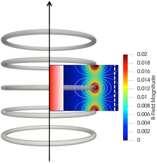
Figure 1. A schematic of a magnetic picket fence plasma system and simulation domain. The schematic shows the contours of magnetic field magnitude and magnetic field lines from the coils without the presence of plasma. The plasma injection region in the central part of the picket fence is shown in graded red and the loss boundary is shown at the right side of the simulation domain as a dotted line.

Method

In the present work, PIC simulations were used to investigate this boundary layer as a function of plasma pressure and ion mass with a spatial resolution beyond electron gyroradius while incorporating the global equilibrium structure. The exploration led to the discovery of a localized electric field at the electron gyroradius scale that transforms our understanding of plasma diamagnetic effects. Further details of the ECsim code and simulation method are given in the Supplementary Material.

Figure 1 shows a schematic of a magnetic picket fence system used in the simulation. It consists of series of circular coils arranged along the vertical axis with opposite coil current direction between adjacent coils. These coils produce zero magnetic field near the central region near the axis and form a magnetic field wall near the coils. The magnetic picket fence was proposed by Tuck in 1954 as a magnetic confinement system to produce thermonuclear fusion reactions (Tuck, 1958). The picket fence is one of the magnetic confinement systems called “magnetic cusps,” that are known to be stable against many of plasma instabilities (Berkowitz et al., 1958; Krall and Trivelpiece, 1973). In this report, the magnetic picket fence system was chosen for the following reasons.

1. Perfect magnetic field shielding by plasma diamagnetism has been experimentally observed in various magnetic cusp systems designed for fusion energy research (Spalding, 1971; Kitsunezaki et al., 1974; Haines, 1977; Pechacek et al., 1980). As such, the magnetic cusp system is well-suited to investigate diamagnetic effects of plasma. In addition, the magnetic field configuration of the picket fence is topologically identical to the dayside Earth magnetosphere with the convex curvature of the Earth's magnetic field facing the solar wind as well as the magnetic fields of sunspots (Spalding, 1971; Berchem, 1990; Kallenrode, 2004).

2. Due to their favorable magnetic field curvature, magnetic cusp systems have been shown to be stable against most, if not all, of macroscopic plasma instabilities in theory. This is because plasma must do work compressing the magnetic field if it expands at the boundary since the magnetic field is curved into the plasma on every surface. The lack of plasma instabilities in magnetic cusp systems has also been reported in many past experiments. This allows the simulation of underlying equilibrium to reach steady-state or at least quasi-steady state in a couple of plasma transit times, as determined by the slower species, i.e., ions.

3. A magnetic picket fence can be simulated with the periodic boundary condition in the axial direction. Most proposed fusion reactor configurations based on magnetic cusp system utilize many pairs of magnetic coils to provide sufficient reactor volume and needed confinement (Dolan, 1994). In the case of a magnetic picket fence utilizing many pairs of coils along the axial direction, the periodic boundary condition is a good approximation in the central region of the picket fence as shown in Figure 1. In the present study, a set of 27 coils are used in the simulation to provide the external magnetic field that is nearly periodic along the symmetric axis with 3 coils in the middle are inside the simulation domain as shown in Figure 1. In addition, the plasma refueling can be achieved by injection from the both ends to achieve steady-state operation, corresponding to volumetric plasma injection near the axis used as in the simulation.

For the study reported, we utilize a fully kinetic description of the equilibrium between plasma and magnetic field, where both electrons and ions are followed as particles interacting via electric and magnetic fields generated by the particles themselves as well as by the coils. The approached followed is the electromagnetic particle in cell (PIC) method. The full set of Maxwell's equations is discretized on a grid where particle moments are collected via first order basis spline interpolation to calculate the sources for Maxwell's equations. In the present paper, we utilized the Energy Conserving semi-implicit method (ECsim) in its cylindrical implementation called ECsim-CYL (Lapenta, 2012, 2017; Gonzalez-Herrero et al., 2019) based on azimuthal symmetry of magnetic picket fence system. The ECsim-CYL solves the field equations in two-dimensional (2D) cylindrical coordinates using a finite volume method. For the particles, it solves all three components of velocity vectors, while only keeping radial and axial coordinates of particle positions. The numerical algorithm of ECsim-CYL has been tested previously for accuracy and convergence (Gonzalez-Herrero et al., 2019).

We utilized the ECsim-CYL code to investigate the plasma diamagnetic effects for the following reasons. The ECsim-CYL conserves the system energy precisely down to machine precision even when the grid and time resolution severely under-resolve the electron plasma frequency or the electron Debye length. This energy conservation allows the simulation to operate without any artificial smoothing. While the field or the particle moment smoothing helps with noise and numerical stability, the use of smoothing leads to the violation of energy conservation and may disrupt the diamagnetic boundary layer leading to an artificially greater layer thickness caused by numerical effects rather than physical effects. Though, in principle, it is possible to avoid the under sampling of electron plasma frequency or Debye length, the numerical cost can be very high, about a factor of 100 or more for the plasma parameter spaces as shown in Table 1. This is because the Debye length is about a factor of 10 smaller than the electron gyroradius. This additional computational cost needs to be multiplied by each dimension, leading to a factor of 100 increase in 2D cylindrical geometry. On the other hand, the implicit PIC codes, such as ECsim, have successfully demonstrated the ability to resolve critical electric field generation regarding charge separation between electrons and ions even when they are under sampling the Debye length (Gonzalez-Herrero et al., 2019). Considering that each run in Table 2 already requires 10,000–150,000 CPU hours to generate an equilibrium solution, the use of the energy conserving algorithm of ECsim was critical to resolve electron gyroradius scale physics in the boundary layer with built-in energy conservation. It is noted that the system energy is conserved to machine precision at all resolutions reported.

TABLE 1

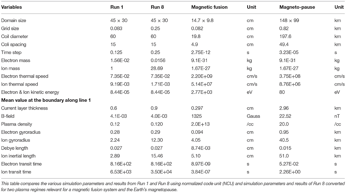
Table 1. Summary of simulation parameters and results.

TABLE 2

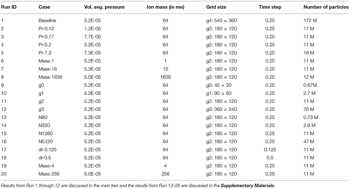
Table 2. Summary of simulation runs with key parameters.

The results from the ECsim code are presented using normalized code units (NCU) that are non-dimensional. The use of NCU allows the simulation results to be converted to various physical systems over a wide range of parameters. As such, we provide two physical examples where the results from the single simulation are converted to plasma parameters relevant to magnetic fusion devices and the Earth's magnetopause as shown in Table 1. In ECsim, time is normalized to the ion plasma frequency, ω_pi, determined by the reference plasma density n₀, as ω_pi = (n₀/m_i)^0.5, where ω_pi is the ion plasma frequency and m_i is the ion mass in NCU. Electron plasma frequency is defined similarly, as ω_pe = (n₀/m_e)^0.5, where ω_pe is the electron plasma frequency and m_e is the ion mass in NCU. Velocities are normalized to the speed of light that is set at 1. Distances are normalized to the ion inertial length, as d_i = c/ω_pi. Separately, the charge of electrons and ions is set at 1 and the permittivity and permeability of free space, and Boltzmann coefficient are also set at 1 in NCU. Details of the unit conversion between the NCU and the physical system are provided in the Supplementary Materials.

Each simulation begins with plasma injection of electrons and ions from the center of the picket fence to achieve the preset plasma pressure and ends when the equilibrium reaches quasi-steady state as shown in Figure 2. The red graded region in Figure 1 shows the area of volumetric plasma injection. In NCU with the length scale normalized to ion inertial length, the size of the simulation domain is 45 in radius and 30 in height or axial length, as shown in Figure 3d, while the injection region is 9 in radius and 30 in height. Coils in the picket fence have a diameter of 60 and the spacing between two adjacent coils is 15. During initialization, ions and electrons are injected with the same temperature with an electron thermal velocity of 7.35 × 10⁻² times the speed of light in NCU. The ion thermal velocity, on the other hand, is adjusted as a function of ion mass to maintain the same temperature for both species. A typical time step is 0.25/w_pi, during which a thermal electron travels 1.84 × 10⁻²/d_i and a thermal ion travels 2.3 × 10⁻³/d_i in NCU. Once injected, the plasma expands and fills the picket fence system while interacting with the externally applied magnetic field. During expansion, the plasma expels a magnetic field from the plasma and forms a boundary. The temporal duration of the injection phase is 8,000/w_pi, corresponding to 10 times the electron transit time or 1.2 times the ion transit time for the ion mass of m_i = 64 m_e. The transit time is defined as the time for thermal ions and electrons to move across one coil diameter. The injection is conducted incrementally for 160 times during the initialization phase with an equal amount of plasma injections leading to gradual increases in the total kinetic energy of the plasma in the picket fence and plasma diamagnetic effects as shown in the top row of Figure 2. Incremental injection is used to build up plasma pressure in the picket fence gradually without generating shocks or significant plasma flow, to investigate the quiescent equilibrium between the static plasma pressure and magnetic field pressure.

FIGURE 2

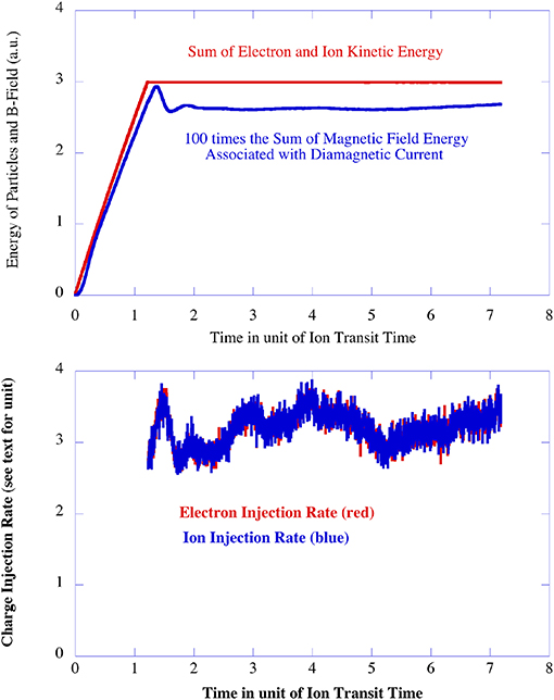
Figure 2. A temporal setup showing the initialization phase and the steady-state phase in the simulation using a unit of ion transit time across the coil diameter of the picket fence. The top row shows the sum of particle kinetic energy in the simulation domain and the sum of magnetic field energy associated with diamagnetic current by the plasma multiplied by 100. The bottom row shows temporal variation of plasma injection rates for electrons and ions to sustain the constant total charge and total particle kinetic energy in the system. The results are from Run 4.

FIGURE 3

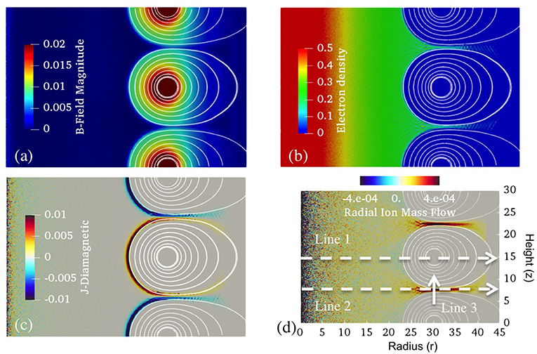
Figure 3. Steady-state equilibrium profiles. Equilibrium profiles show contours of (a) magnitude of B-field, (b) electron density, (c) diamagnetic current density, and (d) radial ion mass flow with magnetic field lines from Run 1 in Table 2. Three lines of interest are defined in (d) for further analysis with Line 1 (r = 0–45 at z = 15), Line 2 (r = 0–45 at z = 7.5), and Line 3 (r = 30, z = 4–11).

Once the preset plasma pressure is reached in the picket fence, the initialization phase is complete and the system is relaxed toward a steady-state, as shown in Figure 2. During the steady-state phase, plasma is maintained by incremental injection in the same central region of the picket fence to replenish the loss of plasma from the picket fence to the loss boundary at the right end of the simulation domain. The loss boundary is simulated as an absorbing wall for particles and electromagnetic waves, shown as a dotted line in Figure 1. It is located at r = 42, away from the coils at r = 30 to prevent the presence of the wall from affecting plasma equilibrium inside the picket fence. Nominally, the injection rate to sustain the plasma during the steady-state phase is ~18 times lower than the injection rate during the initialization phase. For example, a charge injection rate of ~ 3 per 22.5/w_pi is utilized to maintain a constant total charge of 1.89 × 10⁴ in the picket fence system for Run 1 in Table 2 during the steady-state. This injection rate corresponds to a particle confinement time of 1.1 × 10⁵/w_pi, equivalent to ~135 electron transit time or ~17 ion transit time. While the injection rates for ions and electrons are allowed to vary from each other while replenishing their respective charge loss, the plasma loss quickly satisfies the ambipolar condition with equal loss of electrons and ions from the picket fence to the absorbing wall as shown in the bottom row of Figure 2. On the other hand, plasma injection during the steady-state phase requires more kinetic energy per injected particles compared to plasma injection during the initialization phase by a factor of 2.5–3. This is equivalent to the energy confinement time of the system being 2.5–3 times shorter than the particle confinement time. A shorter energy confinement time is typical in most plasma systems as higher energy particles leave the systems faster than lower energy particles.

Nominally, the simulation is conducted for a minimum of 2.2 times the ion transit times after the initialization phase to ensure steady-state. By then, all equilibrium properties such as plasma density, current density, plasma pressure, plasma flow and magnetic field are nearly constant in space and time. As shown in M1 and M2 (Movies in Supplementary Materials), the location and the width of the boundary layer are constant with less than one to two pixels variation. The M1 is from Run 8 in Table 2 that covers 7 ion transit times from beginning to an end and the M2 is from Run 1 in Table 2 that covers to 3.5 ion transit time from the beginning to an end. Note that the sudden changes in radial ion mass flow, shown in the movies, are related to transition from the initialization phase to the steady-state phase, which involves change in plasma injection rate by a factor of ~18. For the present study, we have conducted systematic studies of equilibrium between the plasma and magnetic field as a function of plasma pressure and ion mass for a constant electron mass. In addition, several additional tests were conducted to ensure the numerical convergence with variation in grid size, time step, and number of simulation particles. Table 2 summarizes the key parameters used in the simulations.

In summary, plasma dynamics in the magnetic picket fence system has been simulated using a fully kinetic PIC code to investigate diamagnetic effects. The simulations utilize the cylindrical symmetry in the angular direction and the periodic boundary condition in axial direction while preserving a dipole nature of the magnetic field in the simulation. A steady-state equilibrium is produced by injection of the plasma in the central part of the picket fence and the plasma loss boundary that absorbs ions and electrons that leak out of the picket fence system, as shown in Figure 1. It is noted that fully a kinetic PIC simulation of the diamagnetic current layer requires significant High Performance Computing (HPC) resources even in the simple geometrical setup of an axisymmetric magnetic picket fence system. Typical runs employ between 300 and 1,200 CPUs and require between 10,000 and 150,000 CPU hours to simulate the steady-state equilibrium while resolving electron gyroradius with satisfactory numerical convergence.

Results

Steady-State Equilibrium

Figure 3 shows the steady-state equilibrium profile of a magnetic picket fence with a sharp boundary between plasma and magnetic field from Run 1 in Table 2. From right to left, the magnetic field exhibits rapid decay across the boundary, leading to a field-free plasma region in the picket fence, as shown in Figure 3a. From left to right, the electron density profile exhibits similarly rapid decay across the boundary, leading to a plasma–free magnetic field region near the magnetic coils, as shown in Figure 3b. Across the boundary, layers of highly localized current are formed from plasma gyromotion separating plasma and magnetic field, as shown in Figure 3c. In addition, collimated ion flows are formed in the funnel-shaped cusp region, resulting in plasma leakage via the gap between the opposing sign of current layers, as shown in Figure 3d. For further analysis, three lines of interest are defined in Figure 3d to describe the boundary between plasma and magnetic field, as described in the Method section. While exhibiting distinctively different equilibrium properties along Lines 1, 2, and 3, the different regions of equilibrium are interconnected by plasma motion and magnetic field, highlighting the necessity of incorporating the global equilibrium structure when investigating boundary layers.

Figure 4 shows steady-state equilibrium profiles as a function of volume averaged plasma pressure for Runs 2, 3, 4, and 5 in Table 2 to investigate the change in equilibrium from plasma pressure change. The top row shows magnitude of magnetic field contours with magnetic field lines drawn to highlight the change in boundary location. The second row shows plasma diamagnetic current density (note that the direction of diamagnetic current is in and out of the plane), with the third row showing electron density and the fourth row showing ion mass flow in a radial direction. Along Line 1 as defined in Figure 3d, the boundary between plasma and magnetic field exhibits similar behavior for all four values of pressure. The increase in plasma pressure is balanced by the compression of the magnetic field. The boundary, marked by localized current layers moves toward the higher magnetic field region near the coils and the thickness of the current layer decreases. In comparison, there are significant differences in equilibrium along Lines 2 and 3. For pressures of 1.2 × 10⁻⁶, 7.7 × 10⁻⁶, and 5.2 × 10⁻⁵ in NCU, the plasma is still bounded by the magnetic wall of the picket fence. At these pressures, diamagnetic current layers converge toward narrow gaps in the cusp region coinciding with collimated ion flow. When the pressure is increased to 7.3 × 10⁻⁵ in NCU, the magnetic wall fails along Line 2. While the current layers still converge toward each other, the gap between them is no longer narrow, with significantly wider density profile along Line 3 and increased radially outward ion flow.

FIGURE 4

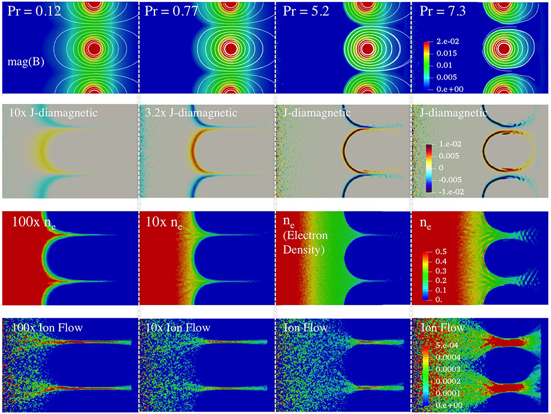
Figure 4. Steady-state equilibrium profiles as a function of plasma pressure. Equilibrium profiles show magnetic field magnitude (top row), diamagnetic current density (second row), electron density (third row), and radial ion mass flow as a function of plasma pressure (fourth row) in the picket fence for four different volume averaged pressure values of 1.2 × 10⁻⁶ (First column from the left). 7.7 × 10⁻⁶ (second column), 5.2 × 10⁻⁵ (third column) and 7.3 × 10⁻⁵ (fourth column) from Runs 2, 3, 4, and 5 in Table 2. The current, density and flow profiles from the pressures of 7.7 × 10⁻⁶ and 5.2 × 10⁻⁵ are multiplied by different factors as noted in plots to utilize the same color scales shown on the fourth column.

Several features of the steady-state equilibrium in a magnetic picket fence in Figures 3, 4 can be explained in a gross way with the standard MHD model. Equation (1) shows the Momentum transport equation of the standard MHD model (Krall and Trivelpiece, 1973).

$\begin{array}{ll}\rho \left(\frac{\partial V}{\partial t}+V·\nabla V\right)=\frac{J\times B}{c}-\nabla p& (1)\end{array}$

where ρ is the mass density of plasma, V is the plasma flow velocity, J is the current density, B is the magnetic field strength, c is the speed of light and p is the plasma pressure. In a steady-state equilibrium, the first term on the left-hand side (lhs) becomes zero, leading to the relationship known as the pressure balance equation among plasma flow, current, magnetic field, and plasma pressure.

Along Line 1, the pressure balance between the plasma and magnetic field forms the boundary with diamagnetic current layers to match the change in magnetic field without plasma flow. With increasing plasma pressure, the boundary moves to the higher B-field region as the plasma works against the magnetic field that is compressible. Since the boundary layer thickness depends on the gyromotion of the plasma, the layer thickness decreases with increasing plasma pressure as previously discussed. In comparison, the pressure gradient along Line 2 generates radially outward plasma flow from the central part of magnetic picket fence toward magnetic cusp openings between two adjacent coils as shown in Figures 3, 4. Past the magnetic cusp openings, the plasma flow then decreases as the magnetic flux expands and the plasma density decreases. Along Line 3, the magnetic field decreases in the plasma region with increasing plasma pressure due to the diamagnetic effects. If the plasma pressure becomes sufficiently high, the magnetic field inside the narrow gap becomes zero as the diamagnetic current provides complete shielding of the magnetic field by plasma. A further increase in the plasma pressure moves the boundary toward the coils similar to the boundary movement along Line 1, opening up the gap and leading to rapid leakage of plasma. Based on the similarity of magnetic field topology, the boundary layers along Line 1 and Line 3 correspond to the magnetopause and sunspot boundary, while collimated plasma flow along Line 2 corresponds to plasma loss to Earth's polar cusp region.

Equilibrium as a Function of Ion Mass

Figure 5 shows plasma profiles in steady-state equilibrium for four different ion masses of m_i = m_e, 16 m_e, 1,836 m_e from Runs 6, 7, 8, and m_i = 64 m_e from Run 4 in Table 1. This study investigates the different roles of electrons and ions in determining equilibrium and boundary layer structure using a mass ratio between electrons and ions as a functional variable. The electron mass is kept constant and the ion mass is varied with the same temperature between electrons and ions. This results in an increase of ion gyroradius with respect to electron gyroradius. For example, the ion gyroradius for m_i = 1,836 m_e is 43 times larger than the ion gyroradius for m_i = m_e. The top row of Figure 5 shows electron density profiles. The second row shows electron diamagnetic current density, and the third row shows ion diamagnetic current density. The radial ion flows are shown in the fourth row.

FIGURE 5

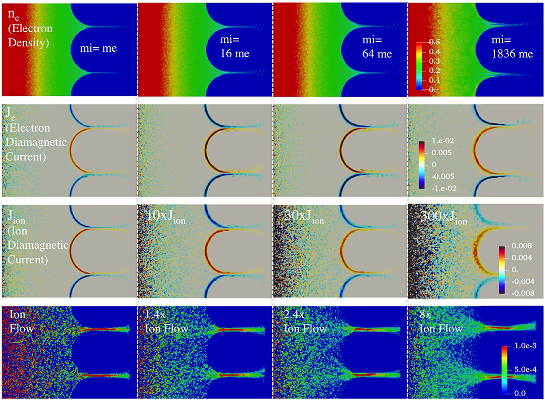
Figure 5. Steady-state equilibrium as a function of ion mass. Equilibrium profiles show electron density (top row), electron diamagnetic current density (second row), ion diamagnetic current density (third row) and radial ion mass flow (fourth row) for 4 different ion masses of m_i = m_e (first column from the left, from Run 6), m_i = 16 m_e (second column, from Run 7), m_i = 64 m_e (third column, from Run 4) and m_i = 1,836 m_e (fourth column, from Run 8). To fit in the same color scales shown on the fourth column, the ion diamagnetic current density and ion flow are multiplied by different factors as noted in plots to utilize the same color scales shown on the fourth column.

The main finding illustrated in Figure 5 is that the equilibrium profiles between the plasma and magnetic field remain nearly identical in their shape when the ion mass and ion gyroradius are varied by a factor of 1,836 and a factor of 43, respectively. For example, the electron diamagnetic current layer occurs at the same location in space with only minor variation in its thickness. In terms of magnitude, electron density and electron diamagnetic current exhibit minimal change with ion mass variation. It is noted that the ion density is not plotted since the ion density is nearly equal to the electron density with the difference between the two is at least 2–3 orders of magnitude smaller than the electron density in the entire domain for all cases. In contrast, there are significant decreases in ion diamagnetic current by a factor of 100 or more between m_i = m_e and m_i = 1,836 m_e, while the ion outward flow in the gap region between the adjacent coils decreases by 8 times along Line 3 (see Figure 3). These results were unexpected and prompted further investigation.

Figure 6 shows equilibrium profiles of radial electric field (top row) and axial electric field (bottom row) which can shed light on the unexpected finding from Figure 5 for the same set of runs. Along Line 1, there is little electric field in the case of m_i = m_e, consistent with the equal gyroradius of electrons and ions. In comparison, a localized electric field is formed and intensifies at the boundary with increase in ion mass to m_i = 16, 64, and 1,836 m_e. The direction of the electric field is radially inward, thus in the direction of pushing ions from the boundary to the plasma region. With ions being pushed radially inward at the boundary, the electric field limits ion excursion into the magnetic field region, which in turn reduces the thickness of the boundary layer. The electric field also disrupts ion gyro-motion at the boundary leading to decreased ion contribution to the plasma diamagnetic current. In addition, the electric field intensity increases with ion mass in order to balance the larger ion gyroradius for heavier ions. While Line 1 is used to describe the role of the localized electric field, the presence of the electric field is seen on the entire surface of the boundary. By comparing the radial and axial electric field, it is shown that the direction of the electric field is normal to the magnetic field line and inward to the plasma region. As this localized electric field at the boundary could explain the results from Figure 5, critical questions are the origin of the electric field and how to quantify its intensity.

FIGURE 6

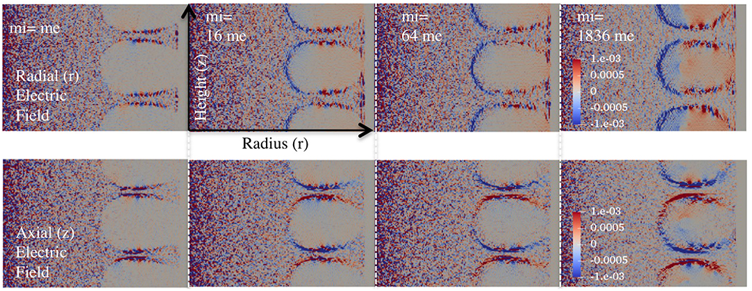
Figure 6. Steady-state equilibrium profiles of electric field as a function of ion mass. Equilibrium profiles show electric field in the radial direction (Top row) and axial direction (Bottom row) for the same ion masses from Runs 4, 6, 7, and 8 as in Figure 5.

Analysis and Discussion

To investigate the origin of the localized electric field, equilibrium profiles along Line 1 are examined in detail in Figure 7 for key plasma parameters in Equation (1). In order to suppress numerical noise related to the use of discrete particles in the PIC simulation, the plot utilizes averaging of 20 steady-state plasma profiles, as discussed in the Method section. Figures 7A–C show equilibrium profiles from Run 1 and Figure 7D shows ion diamagnetic current profiles as a function of grid resolution from Runs 1, 9, 10, 11, and 12 in Table 2. As shown in Figure 7A, the boundary layer exhibits rapid change in plasma density, magnetic field and the diamagnetic current when the thickness of the current layer is ~0.6 as measured by full-width-half-maximum (FWHM). In addition, the radial profile reveals the occurrence of an electric field and its location with respect to the current layer. Figure 7B shows the electron and ion density profile in a semi-log plot, exhibiting exponential decay of both ion, and electron density across the boundary layer. Figure 7C compares the radial electric field and the gradient of ion pressure divided by ion density showing that the electric field develops at the boundary as the ion pressure decreases. While detailed simulation parameters and results are summarized in Table 1, some relevant values are given here for Run 1. In NCU, the simulation utilizes an electron thermal velocity of 7.35 × 10⁻² times the speed of light with an electron mass of 1/64 and an ion thermal velocity of 9.2 × 10⁻³ times the speed of light with an ion mass of 1, with the speed of light and charge of electrons and ions normalized to 1. As shown in Figure 7A, a mean value of magnetic field magnitude is 4.1 × 10⁻³ in the current layer. This leads to the thermal electron gyroradius of 0.28 and the ion gyroradius of 2.24 since the gyroradius is given as the thermal velocity multiplied by the particle mass and the inverse of magnetic field in NCU. Therefore, the current layer thickness of 0.6 corresponds to approximately twice the electron gyroradius and a quarter the ion gyroradius.

FIGURE 7

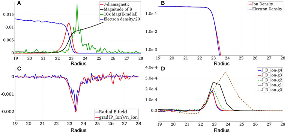
Figure 7. Radial profiles along Line 1 during steady-state equilibrium: (A) Magnitude of B-field and E-field multiplied by 10, Diamagnetic current density and Electron density divided by 20, (B) Electron and Ion density, (C) Radial electric fields and gradient of ion pressure divided by ion density, and d) Ion diamagnetic current density as a function of grid resolution. For plots (A–C), the results are from Run 1 with the grid resolution of 540 × 360. For plot (D), grid resolutions of g0 (45 × 30). g1 (90 × 60), g2 (180 × 120), g3 (360 × 240), and g4 (540 × 360) are used for numerical convergence investigation from Runs 1, 9, 10, 11, and 12 from Table 2.

During the analysis to quantify the electric field intensity, we have also discovered the importance of spatial resolution for PIC simulation, as shown in Figure 7D. Here we conducted a series of convergence tests with respect to the grid resolution from g0 (45 × 30) to g1 (90 × 60), g2 (180 × 120), g3 (360 × 240), and g4 (540 × 360) corresponding to the grid size varying from 3.6, 1.8, 0.9, 0.45, and 0.30 times the electron gyroradius at the boundary. Figure 7D shows ion diamagnetic current density as a function of grid resolution. The simulation reaches a converged solution for g3 and g4, while g2 results seem to be reasonably close to the converged solution with respect to ion diamagnetic current density. On the other hand, without sufficient grid resolution, such as in the g0 and the g1 cases, numerical inadequacy leads to over-estimation of ion diamagnetic current density and its layer thickness in the boundary layer.

The results shown in Figures 7A–C are unexpected and outside the standard MHD model, whose solution of the current layer does not include the electric field. Instead, we compare the results with the equation known as generalized Ohm's law, including the Hall term and a scalar pressure, which relates the current to the electric field, as shown in Equation (2) (Biskamp, 2000).

$\begin{array}{ll}E=-\frac{V_i\times B}{c}+\frac{1}{ne}\times \frac{J\times B}{c}-\frac{\nabla p_e}{ne}& (2)\end{array}$

where E is the electric field, V_i is the velocity of ions, n is the plasma density, e is the electron charge and p_e is the pressure of electrons. It should be remarked that the simulations do not use this approximation. Equation (2) is used only to interpret the results. Within this scope, we can then simplify the pressure tensor with a scalar pressure and ignore the electron inertial terms. Furthermore, time varying terms are ignored in Equation (2) as we are interested in steady-state equilibrium. To focus on the most important terms, it is instructive to consider the consequences of assuming the limit where the electron inertia terms, the plasma resistivity term and other higher order terms such as off-diagonal pressure tensor terms are ignored as well as the difference between the electron density and the ion density. First, we note that the first term on the right-hand side (rhs) can be ignored at the boundary along Line 1 since there is no plasma mass flow as shown in Figure 1. We can then utilize Equation (1) to replace the J × B term, the second term on the rhs with the total pressure gradient reducing Equation (2) into a simple relation between the electric field and the ion pressure at the boundary.

$\begin{array}{ll}E=\nabla p_i/ne\text{ or},E=k{T}_i\nabla n_i/ne& (3)\end{array}$

where p_i is the pressure of ions, k is the Boltzmann coefficient, T_i is the ion temperature and n_i is the ion density.

This relationship between the electric field and the ion density gradient where the ion density gradient scale length is on the order of electron gyro-radius is the key discovery of the present study. Since the electric field intensity is proportional to the ion density gradient, it highlights the importance of fully resolving length scale down to the electron gyroradius in determining ion dynamics at the boundary. An approximate solution of this relationship can be expressed as n_i ~ n₀exp (eE₀(r-r_b)/kT_i), where n₀ is the ion density at the boundary location at r = r_b and E₀ is mean electric field value in the boundary layer. The observed exponential decay of ion density shown in Figure 7B agrees with this solution. Finally, Figure 7C shows an agreement between the radial electric field and the gradient of ion pressure divided by the ion density, as shown in Equation (3).

To further understand the role of the electric field, Figure 8 compares single particle ion trajectories in the equilibrium from Run 1 with and without the electric field along Lines 1 and 2 with green dots representing origins of their trajectories. All ions begin their motion with the same velocity vector angled at 15 degrees between radial velocity and axial velocity, and their kinetic energy equal to twice the kinetic energy of plasma injection during the initialization phase. As shown in Figures 8a,b, ion motions exhibit sharp reflection at the boundary due to the presence of the electric field. In comparison, ions would penetrate significantly deeper across the boundary layer if the electric field is ignored, as shown in Figures 8c,d. Along Line 1, the sharp reflection of ions at the boundary is consistent with the exponential ion density decay, with the characteristic decay length comparable to electron gyroradius. The electric field also contributes to the ion flow collimation along Lines 2 and 3, with a width of ion flow significantly less than ion gyroradius, while suppressing plasma leakage, as shown in Figure 8b. Without the electric field at the boundary, the width of the ion flow would be significantly wider, as shown in Figure 8d. As such, this localized electric field may play a significant role in suppressing the plasma loss in magnetic cusp systems. Previously, the plasma loss rate of magnetic cusp device was conjectured to be proportional to the width of the cusp opening (Berkowitz et al., 1958; Grad, 1961; Spalding, 1971; Kitsunezaki et al., 1974; Hershkowitz et al., 1975; Haines, 1977; Pechacek et al., 1980). Since the minimum width of the cusp opening across Line 3 is twice the thickness of boundary layer along Line 1, the reduced plasma loss across the cusp opening due to the electric field is also consistent with the electron gyro-radius scale boundary layer.

FIGURE 8

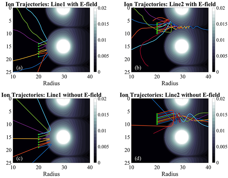
Figure 8. Ion trajectories in the steady-state equilibrium with and without an electric field from Run 1. Panels (a,b) show ion trajectories with the self-consistent electric field and magnetic field from the simulation. Panels (c,d) show ion trajectories calculated with only the magnetic field to highlight the role of the electric field at the boundary in determining the thickness of the boundary layer and the plasma flow collimation.

The results from Figure 8 show that the main role of the electric field at the boundary is to limit ion excursion at the boundary, which in turn limit charge separation between electrons and ions, as shown in Figure 7B. As the ion excursion is suppressed at the boundary, the ion density decreases rapidly at the boundary. This leads to the decrease of ion diamagnetic current with the ion diamagnetic current layer thickness comparable to the electron diamagnetic current layer thickness, as shown in Figure 3. At the same time, the gradient of ion density or ion pressure term becomes significant, which gives a rise to the electric field at the boundary as shown in Figure 7C and Equation (3). Therefore, this electric field can be described as the self-consistent field since it occurs to prevent additional charge separation beyond the generation of the electric field leading to the electron gyroradius scale boundary layer. It is noted that the results from Figure 8 provides a clear explanation for the previously unresolved rapid formation of collimated ion flow observed since the ion collimation is caused by the self-consistent electric field rather than ion gyromotion (Hershkowitz et al., 1975). It is noted that spatially localized electric fields and their role in limiting ion motion has been investigated in the boundary of tokamak magnetic confinement devices (Itoh and Itoh, 1988; Shoucri et al., 2004). In these works, the spatial scale of boundary layer and electric fields was found to be ion gyro-radius rather than electron gyro-radius as the deviation of electron motion from the magnetic flux surface was ignored. While the presence of a strong guiding magnetic field and the concave curvature of magnetic field lines at the boundary may play significant roles in determining the length scale of boundary layer and localized electric fields, it may be worthwhile to extend the previous works to the electron gyro-radius scale by allowing the decoupling of electron motion from the magnetic surface.

Our central result is that diamagnetic effects of plasma can produce electron-scale boundary layers across which current, density and magnetic field exhibit sharp transition on electron gyroradius scale length. This discovery comes at a fortuitous moment when the recently launched Magnetospheric Multiscale (MMS) mission has the capability to capture electron scale plasma dynamics both as a function of time from the high cadence of its instrumentation and space because of the short distance between its four spacecraft. It should therefore be possible in principle to observe our predicted structures. For example, Burch et al. reported an observation of electron scale current layers in the electron diffusion region of magnetic reconnection sites during magnetopause crossings by MMS spacecraft and identified the critical role of electron dynamics and localized electric fields in triggering magnetic reconnection (Burch et al., 2016). Localized electric fields have been reported also from previous missions such as Cluster (Wygant et al., 2005) and observed in simulation studies of the separation of scale of electrons and ions in reconnection (Zenitani et al., 2013) where the orbit of ions and electrons and the role of the pressure term is similar to the one reported here (Wang et al., 2016). Electron scale current layers have also been observed in the magnetosheath as part of the turbulent cascade with the observation of the electron jets in the absence of ion reconnection signature. (Phan et al., 2018). In addition, small scale magnetic holes produced by diamagnetic effects have been observed where the magnetic hole exhibits electric and magnetic field boundary structures on the order of ~30 km compared to the ion gyroradius of 100–1,000 km (Goodrich et al., 2016). Finally, the electron scale diamagnetic current layer has also been observed with the current produced predominantly by the divergence of pressure tensor near a magnetic reconnection region (Rager et al., 2018). While exact mechanisms producing such electron scale current layers and field structure requires further investigations, the electron scale diamagnetic current layer discovered in our simulation could be a possible source of these electron scale plasma structures.

Summary and Conclusion

The fully kinetic first principles simulation resolving electron gyroradius scale length reported here led to the discovery of a localized and self-consistent electric field that plays a critical role in the boundary layer marked by a diamagnetic current between the plasma and surrounding magnetic fields. This electric field arises from the ion density or pressure gradient at the boundary and its main role is to limit charge separation between electrons and ions. By suppressing ion excursion across the boundary, the electric field leads the current layer thickness to the length scale of the electron gyroradius, the smallest and most fundamental length scale in the magnetic properties of plasma, instead of the much larger ion gyroradius. The electric field also affects plasma transport across the boundary by collimating plasma flow in the cusp region flow and reducing plasma leakage.

The localized electric field highlights the necessity to incorporate electron gyroradius scale physics in future studies aimed at advancing our understanding of fusion device performance, the magnetosphere and sunspots. In the case of magnetic cusp fusion devices, the findings from the present study encourage the resumption of research into magnetic cusp devices as potential thermonuclear fusion energy reactors. Magnetic cusp systems, in addition to their proven plasma stability and engineering simplicity, are one of the few magnetic fusion devices that allow direct injection of a charged particle beam into the central region (Krall et al., 1995; Park et al., 2015). The use of an electron beam may allow control of the electric field at the boundary toward the further improvement of plasma confinement in conjunction with flow collimation (Dolan, 1994). A numerical capability to accurately calculate the electric field offers the tantalizing potential to improve the performance of magnetic cusp devices toward net fusion energy generation. While the present work is focused on systems where the diamagnetic current layer separates a field-free plasma and a plasma-free magnetic field, the localized electric field may also play a role in plasma equilibrium and confinement at the boundaries of other fusion devices, such as the tokamak, stellarator, magnetic mirror, and Field Reversed Configuration (FRC). This is because the diamagnetic current and steep pressure gradient occur in the boundary layers of these devices where a localized electric field in the electron gyro-radius scale may play an important role in determining plasma transport. However, it is noted that unlike magnetic picket fence, these fusion systems are inherently three-dimensional systems and will require significantly higher computational resource to investigate electron gyro-radius scale physics. In the case of the Earth's magnetosphere, incorporating an electron gyroradius scale boundary layer in the quintessential equilibrium between the solar wind plasma and the Earth's magnetic field will provide new insights into magnetic reconnection and plasma turbulence. This is because the gradient scales of the current layer and plasma pressure play a critical role in the reconnection rate and turbulence spectrum in magnetic reconnection and plasma turbulence. Extending experimental and theoretical tools toward electron gyroradius scale phenomena will help to take full advantage of the recently launched MMS mission.

Data Availability Statement

All datasets generated for this study are included in the article/Supplementary Material.

Author Contributions

JP contributed to the conceptualization of the problem, conducted simulations and analysis, and prepared the manuscript. GL contributed to the development of the simulation code, conducted the analysis, and edited the manuscript. DG-H contributed to the development of the simulation code and provided the support for conducing simulations. NK contributed to the conceptualization of the problem and supported the analysis.

Conflict of Interest

The authors declare that the research was conducted in the absence of any commercial or financial relationships that could be construed as a potential conflict of interest.

Acknowledgments

The authors would like to thank Prof. John F. Santarius at Univ. Wisconsin, Madison and Prof. Yong Seok Hwang at Seoul National Univ. of Korea for their helpful discussion on plasma diamagnetic effects and Dr. Alan Roberts at Energy Matter Conversion Corporation and Mr. John Draper at Khon Kaen Univ. of Thailand for their assistance in editing of the manuscript. The initial funding for this work came from the internal corporate research and development funds of Energy Matter Conversion Corporation. This research used computational resources provided by NASA NAS and NCCS High Performance Computing, by Flemish Supercomputing Center (VSC), and by PRACE Tier-0 allocations. This manuscript has been released as a Pre-Print at arXiv (Park et al., 2019).

Supplementary Material

The Supplementary Material for this article can be found online at: https://www.frontiersin.org/articles/10.3389/fspas.2019.00074/full#supplementary-material

References

Alfvén, H. (1942). Existence of electromagnetic-hydrodynamic waves. Nature 150, 405–406.

Google Scholar

Alfvén, H. (1963). Hydromagnetics of the magnetosphere. Space Sci. Rev. 2, 862–870.

Google Scholar

Berchem, J. (1990). Hideo Okuda, a two-dimensional particle simulation of the magnetopause current layer. J. Geophys. Res. 95, 8133–8147.

Google Scholar

Berkowitz, J., Friedrichs, K. O., Goertzel, H., Grad, H., Killeen, J., and Rubin, E. (1958). “Cusped geometries,” in Proceedings of the 2nd United Nations International Conference on Peaceful Uses of Atomic Energy, Vol. 31, 171–197 (Geneva: United Nations)

Google Scholar

Bessho, N., Chen, L. J., and Hesse, M. (2016). Electron distribution functions in the diffusion region of asymmetric magnetic reconnection. Geophys. Res. Lett. 43, 1828–1836.

Google Scholar

Biskamp, D. (2000). Magnetic Reconnection in Plasmas. Cambridge: Cambridge University Press.

Google Scholar

Borrero, J. M., and Ichimoto, K. (2011). Magnetic structure of sunspots. Living Rev. Sol. Phys. 8, 4–98. doi: 10.12942/lrsp-2011-4

PubMed Abstract | CrossRef Full Text | Google Scholar

Braginskii, S. I., and Kadomtsev, B. B. (1959). Plasma Physics and the Problem of Controlled Thermonuclear Reactions, Vol. 3. New York, NY: Pergamon Press.

Google Scholar

Burch, J. L., Torbert, R. B., Phan, T. D., Chen, L. J., Moore, T. E., Ergun, R. E., et al. (2016). Electron-scale measurements of magnetic reconnection in space. Science 352:aaf2939. doi: 10.1126/science.aaf2939

PubMed Abstract | CrossRef Full Text | Google Scholar

Chapman, S., and Ferraro, V. C. A. (1930). A new theory of magnetic storms. Nature 126, 129–130.

Google Scholar

Cowling, T. G. (1957). Magnetohydrodynamics. New York, NY: Interscience.

Google Scholar

Dolan, T. J. (1994). Magnetic electrostatic plasma confinement. Plasma Phys. Control. Fusion 36, 1539–1593.

Google Scholar

Dungey, J. W. (1961). The steady state of the Chapman-Ferraro problem in two dimensions. J. Geophys. Res. 66, 1043–1047.

Google Scholar

Gonzalez-Herrero, D., Micera, A., Boella, E., Park, J., and Lapenta, G. (2019). ECsim-CYL: energy conserving Semi-implicit particle in cell simulation in axially symmetric cylindrical coordinates. Comput. Phys. Commun. 236, 153–163. doi: 10.1016/j.cpc.2018.10.026

CrossRef Full Text | Google Scholar

Goodrich, K. A., Ergun, R. E., Wilder, R., Burch, J., Torbert, R., Khotyaintsev, Y., et al. (2016). MMS Multipoint electric field observations of small-scale magnetic holes. Geophys. Res. Lett. 43, 5953–5959. doi: 10.1002/2016GL069157

CrossRef Full Text | Google Scholar

Grad, H. (1961). Boundary layer between a plasma and a magnetic field. Phys. Fluids 4, 1366–1375.

Google Scholar

Haines, M. G. (1977). Plasma containment in cusp-shaped magnetic fields. Nucl. Fusion 17, 811–858.

Google Scholar

Hale, G. E. (1908). On the probable existence of a magnetic field in sun-spots. Astrophy. J. 28, 315–343.

Google Scholar

Hershkowitz, N., Leung, K. N., and Romesser, T. (1975). Plasma leakge through a low-β line cusp. Phys. Rev. Lett. 35, 277–280.

Google Scholar

Itoh, S.-I., and Itoh, K. (1988). Model of L to H-mode transition in Tokamak. Phys. Rev. Lett. 60, 2276–2279.

PubMed Abstract | Google Scholar

Kallenrode, M.-B. (2004). Space Physics: An Introduction to Plasmas and Particles in the Heliosphere and Magnetospheres. New York, NY: Springer.

Google Scholar

Kitsunezaki, A., Tanimoto, M., and Sekiguchi, T. (1974). Cusp confinement of high beta plasmas produced by a laser pulse from a freely-falling deuterium ice pellet. Phys. Fluids 17, 1895–1902.

Google Scholar

Krall, N. A., Coleman, M., Maffei, K. C., Lovberg, J. A., Jacobsen, R. A., and Bussard, R. W. (1995). Forming and maintaining a potential well in a quasispherical magnetic trap. Phys. Plasmas 2, 146–160.

Google Scholar

Krall, N. A., and Trivelpiece, A. W. (1973). Principles of Plasma Physics. New York, NY: McGraw-Hill.

Google Scholar

Lapenta, G. (2012). Particle simulations of space weather. J. Comput. Phys. 231, 795–821. doi: 10.1016/j.jcp.2011.03.035

CrossRef Full Text | Google Scholar

Lapenta, G. (2017). Exactly energy conserving semi-implicit particle in cell formulation. J. Comput. Phys. 334, 349–366. doi: 10.1016/j.jcp.2017.01.002

CrossRef Full Text | Google Scholar

Park, J., Krall, N. A., Sieck, P. E., Offermann, D. T., Skillicorn, M., Sanchez, A., et al. (2015). High-energy electron confinement in a magnetic cusp configuration. Phys. Rev. X 5:021024.

Google Scholar

Park, J., Lapenta, G., Gonzalez-Herrero, D., and Krall, N. A. (2019). Discovery of an electron gyroradius scale current layer: its relevance to magnetic fusion energy earth magnetosphere and sunspots. arXiv [Preprint]. arXiv:1901.08041.

Google Scholar

Pechacek, R. E., Greig, J. R., Koopman, D. W., and DeSilva, A. W. (1980). Measurement of the plasma width in a ring cusp. Phys. Rev. Lett. 45, 256–259.

Google Scholar

Phan, T. D., Eastwood, J. P., Shay, M. A., Drake, J. F., Sonnerup, B. U. Ö., Fujimoto, M., et al. (2018). Electron magnetic reconnection without ion coupling in earth's turbulent magnetosheath. Nature 557, 202–206. doi: 10.1038/s41586-018-0091-5

PubMed Abstract | CrossRef Full Text | Google Scholar

Rager, A. C., Dorelli, J. C., Gershman, D. J., Uritsky, V., Avanov, L. A., Torbert, R. B., et al. (2018). Electron crescent distributions as a manifestation of diamagnetic drift in an electron-scale current sheet: magnetospheric multiscale observations using new 7.5 ms fast plasma investigation moments. Geophys. Res. Lett. 45, 578–584. doi: 10.1002/2017GL076260

PubMed Abstract | CrossRef Full Text | Google Scholar

Russell, C. T., and Kivelson, M. G., (eds.). (1995). Introduction to Space Physics. Cambridge: University Press.

Google Scholar

Shoucri, M., Gerhauser, H., and Finken, K. H. (2004). Study of the generation of a charge separation and electric field at a plasma edge using Eulerian Vlasov codes in cylindrical geometry. Comput. Phys. Commun. 164, 138–149. doi: 10.1016/j.cpc.2004.06.022

CrossRef Full Text | Google Scholar

Sonnerup, B. U. Ö., and Cahill, L. J. Jr. (1967). Magnetopause structure and attitude from explorer 12 observations. J. Geophy. Res. 72, 171–183.

Google Scholar

Spalding, I. (1971). “Cusp containment,” in Advances in Plasma Physics, Vol. 4, eds A. Simon and W. B. Thomson (New York, NY: Interscience, 79–123.

Google Scholar

Tuck, J. L. (1958). “Review of controlled thermonuclear research at Los Alamos for mid 1958,” in Proceedings of the 2nd United Nations International Conference on Peaceful Uses of Atomic Energy, Vol. 32, 3–25 (Geneva: United Nations).

Google Scholar

Wang, S., Chen, L.-J., Hesse, M., Bessho, N., Gershman, D. J., Dorelli, J., et al. (2016). Two-scale ion meandering caused by the polarization electric field during asymmetric reconnection. Geophys. Res. Lett. 43, 7831–7839. doi: 10.1002/2016GL069842

CrossRef Full Text | Google Scholar

Wygant, J. R., Lysaket, R., Songal, Y., Dombeck, J., McFadden, J., Mozer, F., et al. (2005). Cluster observations of an intense normal component of the electric field at a thin reconnecting current sheet in the tail and its role in the shock-like acceleration of the ion fluid into the separatrix region. J. Geophys. Res. Space Phys. 110:A09206. doi: 10.1029/2004JA010708

CrossRef Full Text | Google Scholar

Zenitani, S., Shinohara, I., Nagai, T., and Wada, T. (2013). Kinetic aspects of the ion current layer in a reconnection outflow exhaust. Phys. Plasmas 20:092120. doi: 10.1063/1.4821963

CrossRef Full Text | Google Scholar