Long-Term Evolution of Highly-Elliptical Orbits: Luni-Solar Perturbation Effects for Stability and Re-entry

This paper investigates the long-term evolution of spacecraft in Highly Elliptical Orbits (HEOs). The single averaged disturbing potential due to luni-solar perturbations, zonal harmonics of the Earth gravity field is written in mean Keplerian elements. The double averaged potential is also derived in the Earth-centered equatorial system. Maps of long-term orbit evolution are constructed by measuring the maximum variation of the orbit eccentricity to identify conditions for quasi-frozen, long-lived libration orbits, or initial orbit conditions that naturally evolve toward re-entry in the Earth's atmosphere. The behavior of these long-term orbit maps is studied for increasing values of the initial orbit inclination and argument of the perigee with respect to the Moon's orbital plane. In addition, to allow meeting specific mission constraints, quasi-frozen orbits can be selected as graveyard orbits for the end-of-life of HEO missions, in the case re-entry option cannot be achieved due to propellant constraints. On the opposite side, unstable conditions can be exploited to target Earth re-entry at the end-of-mission.

Introduction

Highly Elliptical Orbits (HEOs) about the Earth are often selected for astrophysics and astronomy missions, as well as for Earth missions, such as Molniya or Tundra orbits, as they offer vantage point for the observation of the Earth and the Universe (Draim et al., 2002). Moreover, elliptical Geostationary Transfer Orbits are commonly selected to inject spacecraft in geostationary orbit. HEOs guarantees spending most of the time at an altitude outside the Earth's radiation belt; therefore, long periods of uninterrupted scientific observation are possible. In addition, geo-synchronicity is opted to meet coverage requirements, enhanced at the apogee, and optimize the ground station down-link. If the inclination is properly selected, HEO can minimize the duration of the motion inside the eclipses.

This paper, whose preliminary version was presented at the 25th AAS/AIAA Space Flight Mechanics Meeting, in Williamsburg (VA) in January 2015 (Colombo, 2015), investigates the long-term evolution of spacecraft in HEOs through the exploitation and development of semi-analytical techniques. The dynamics of HEOs with high apogee altitude is mainly influenced by the effect of third body perturbations due to the Moon and the Sun, which induces long-term variations in the eccentricity and the inclination, corresponding to large fluctuations of the orbit perigee and the effect of the Earth's oblateness.

The semi-analytical technique based on averaging is an elegant approach to analyze the effect of orbit perturbations. It separates the constant, short periodic and long-periodic terms of the disturbing function. The short-term effect of perturbations is eliminated by averaging the variational equations, or the corresponding potential, over one orbit revolution of the small body. Indeed, averaging corresponds to filtering the higher frequencies of the motion (periodic over one orbit revolution), which typically have small amplitudes (Ely, 2014). The resulting system allows a deeper understanding of the dynamics (Shapiro, 1995; Krivov and Getino, 1997). Moreover, the use of the average dynamics reduces the computational time for numerical integration as the stiffness of the problem is reduced, while maintaining sufficient accuracy compatible with problem requirements also for long-term integrations.

The effect of third body is usually modeled as a series expansion of the potential with respect to the ratio between the orbit semi-major axis and the distance to the third body. In averaged development the potential is usually truncated to the second order. For example, Cook's formulation gives the secular and long-periodic perturbation due to luni-solar perturbation obtained through averaging over one orbit revolution of the satellite (Cook, 1962). It assumes circular orbit for the disturbing bodies and considers only the second term of a/a′, where a and a′ are, respectively, the spacecraft and the disturbing body semi-major axis about the Earth (Blitzer, 1970). However, it does consider the obliquity of the Sun and the Moon over the equator and the precession of the Moon plane due to the Earth's oblateness (in a period of 18.6 years with respect to the ecliptic). For orbits above Low Earth Orbits, considering only the second order is not enough to accurately estimate the effect of luni-solar perturbations. For example, Lara et al. (2012) focused on orbital configurations, such as the Global Navigation Satellite Systems, for which the second order effects of J₂ can be of the same order of magnitude as perturbations due to the P₂ up to P₅ terms in the Legendre polynomials expansion of the third-body's disturbing function. For this reason, some recursive formulations of the third body potential were developed (Cefola and Broucke, 1975; Laskar and Bou, 2010) also for recovering the short periodic effects (El'yasberg, 1967).

In this paper, the single averaged disturbing potential due to luni-solar perturbations is developed in series of Taylor of the ratio between the orbit semi-major axis and the distance to the third body, following the approach by Kaufman and Dasenbrock (1972). The effect of other zonal harmonic of the Earth gravity field is also modeled up to order 6 considering also the $J_2^2$ term (Liu and Alford, 1980). As we want to focus here on the interaction between the terms of the Legendre polynomial of the luni-solar perturbation and the Earth's oblateness, the effect of solar radiation pressure and aerodynamics drag is neglected in this work. The perturbed dynamics is propagated in the Earth-centered equatorial frame by means of the single averaged variation (over the orbit revolution of the spacecraft) of the disturbing potential, implemented in the suite PlanODyn (Colombo, 2016). The long-term evolution of high elliptical orbits is characterized in the phase space of eccentricity, inclination and argument of the perigee with respect to the Earth-Moon plane. Maps of long-term evolution are constructed to assess the maximum and minimum eccentricity attained as function of the initial conditions. Through these maps, conditions for quasi-frozen, or long-lived libration orbits are identified. Recent projects funded by the European Space Agency on the design of disposal trajectories for Medium Earth Orbits (Rossi et al., 2015), Highly Elliptical Orbits and Libration Earth Orbits (Armellin et al., 2014; Colombo et al., 2014b) have demonstrated the possibility of exploiting orbit perturbations for designing of passive mitigation strategies for debris disposal. From the results of these projects, many work stemmed out proposing the use of maps for characterizing conditions for natural re-entry in low Earth orbit (Alessi et al., 2018), medium Earth orbit (Alessi et al., 2016; Daquin et al., 2016; Gkolias et al., 2016; Skoulidou et al., 2017), geostationary Transfer orbit (Srongprapa, 2015), geostationary orbit (Colombo and Gkolias, 2017; Gkolias and Colombo, 2017), and highly elliptical orbit (Colombo, 2015).

Third body perturbations show important effects on the long-term evolution of orbits within the Medium Earth orbit region and above. A relevant contribution to the understanding of high-altitude orbit dynamics was given by Kozai's (1962) analytical theory on secular perturbations of asteroid with high inclination and eccentricity. Assuming one perturbing body on a circular orbit, and considering the second term of the disturbing potential, an analytical solution was found, later named as Kozai-Lidov dynamics (Kozai, 1962; Lidov, 1962), which links the eccentricity of the orbit with the inclination, measured from the perturbing body plane, and the argument of the perigee. Their work was more recently extended to consider the slow variation due to the 4^th term of the potential and highlighting shirking characteristics in the phase space (Katz et al., 2011; Naoz et al., 2013). Always in the line of long term analysis of the third body effect, El'yasberg (1967) derived the double averaged equations of the second term of the disturbing potential and Costa and Prado (2000) continued on the effort by El'yasberg by expanding the derivation of the double averaged potential up to order 8th. Their interest concerned the critical value of the inclination between the perturbed and the perturbing body related to the stability of near-circular orbits. In other words for inclination higher than the critical values, circular orbits get very elliptic, while for lower values the orbit stays nearly circular. In El'yasberg (1967) and Costa and Prado (2000) the double averaging was performed using the orbital elements of the spacecraft as defined with respect to the third body plane. However, when considering both the third body effects of the Sun and the Moon, one has to assume that they orbit on the same plane; this reduce to consider that the 5.1° inclination of the Moon's plane over the ecliptic is equal to zero.

In this work, to guarantee the consistency with the single-averaged approach, we do not make this assumption. The double average variation is here obtained averaging on the fast variable describing the orbital motion of the perturbing body around the Earth as in El'yasberg (1967) and Costa and Prado (2000), but the different inclination of the perturbing bodies planes is retained. The double-averaged disturbing potential is derived in the Earth-centered equatorial reference system. The choice of this system has the advance of allowing the description of the perturbing effect of the Sun and the Moon, considering the actual ephemerides and their inclination with respect to the equator, and accommodating also the inclusion of the effect of the zonal harmonics of the Earth potential, which also affect the motion.

By using the single averaged and double averaged equations presented in this paper, the behavior of quasi-frozen solutions appearing for high inclinations orbits can be reproduced. The choice of representing the maps in terms of inclination and argument of the perigee with respect to the Moon plane is quite appropriate here as we want to study the effects on highly elliptical orbit for which the Moon third body perturbations is the most relevant effect. In addition, to allow meeting specific mission constraints, stable conditions for quasi-frozen orbits can be selected as graveyard orbits for the end-of-life of HEO missions, in the case re-entry option cannot be achieved due to propellant constraints, such as XMM-Newton, which is taken here as practical example. On the opposite side, unstable conditions can be exploited to target an Earth re-entry at the end-of-mission (Jenkin and McVey, 2008; Colombo et al., 2014a). This is the case of the end-of-life of INTEGRAL mission, requiring a small delta-v maneuvers for achieving a natural re-entry assisted by perturbations. In this paper, maps of stable and unstable HEOs are built, to be used as preliminary design tool for graveyard or frozen orbit design or natural re-entry trajectories at the end-of-life. Given the available delta-v on-board, the reachable space of orbital elements can also be identified as in the case of XMM-Newton mission.

Long-Term Orbit Evolution

Orbit Evolution With Single-Averaged Disturbing Potential

To analyze the long-term and secular effect of orbit perturbations, it is convenient to use an averaging approach. In the case the effect of perturbations is conservative, this can be described through a disturbing potential R. In this work we consider the perturbation to the two-body dynamics due to the zonal harmonics of the Earth gravity field, and the third-body perturbation of the Sun and the Moon as

$R=R_{\text{zonal}}+R_{3-\text{Sun}}+R_{3-\text{Moon}}$

The variation of the orbital elements is described through the planetary equations in the Lagrange form (Battin, 1999):

$\begin{array}{l}\frac{da}{dt}=\frac{2}{na}\frac{\partial R}{\partial M}\\ \frac{de}{dt}=\frac{1}{n{a}^{2}e}\left(\left(1-e^2\right)\frac{\partial R}{\partial M}-\sqrt{1-e^2}\frac{\partial R}{\partial \omega }\right)\\ \frac{di}{dt}=\frac{1}{n{a}^2\sin i\sqrt{1-e^2}}\left(\cos i\frac{\partial R}{\partial \omega }-\frac{\partial R}{\partial \Omega }\right)\\ \frac{d\Omega }{dt}=\frac{1}{n{a}^2\sin i\sqrt{1-e^2}}\frac{\partial R}{\partial i}\\ \frac{d\omega }{dt}=-\frac{1}{n{a}^2\sin i\sqrt{1-e^2}}\cos i\frac{\partial R}{\partial i}+\frac{\sqrt{1-e^2}}{n{a}^{2}e}\frac{\partial R}{\partial e}\\ \frac{dM}{dt}=n-\frac{\left(1-e^2\right)}{n{a}^{2}e}\frac{\partial R}{\partial e}-\frac{2}{na}\frac{\partial R}{\partial a}& (1)\end{array}$

that can be written in condense form as

$\begin{array}{ll}\frac{d\alpha }{dt}=f\left(\alpha ,\frac{\partial R}{\partial \alpha }\right)& (2)\end{array}$

where α is here used as the condensed form of the Keplerian elements α = [a e i Ω ω M]^T, where a is the semi-major axis, e the eccentricity, i the inclination, Ω the right ascension of the ascending node, ω the argument of the perigee and M the mean anomaly. Through single averaging operation, the potential can be replaced by the orbit-averaged form of the disturbing function:

$\begin{array}{ll}\overline{R}={\overline{R}}_{\text{zonal}}+{\overline{R}}_{3-\text{Sun}}+{\overline{R}}_{3-\text{Moon}}& (3)\end{array}$

obtained under the assumption that the orbital elements are constant over one orbit revolution of the spacecraft around the central planet. Therefore, the variation of the mean elements is described by:

$\begin{array}{ll}\frac{d\overline{\alpha }}{dt}=g\left(\overline{\alpha },\frac{\partial \overline{R}}{\partial \alpha }\right)& (4)\end{array}$

where now $\overline{\text{α}}$ is the vector of the averaged orbital elements.

Luni-Solar Averaged Potential

For describing the effects of luni-solar third body perturbations, we follow the approach proposed by Kaufman and Dasenbrock (1972). Their approach is summarized in this section as is fundamental to give an insight into the orbital dynamics that is exploited in section Luni-Solar and Zonal Harmonics Maps. The disturbing potential due to the third body perturbation is (Murray and Dermott, 1999):

$\begin{array}{ll}R\left(r,r^{\prime }\right)={\mu }^{\prime }\left(\frac{1}{\left|r-r^{\prime }\right|}-\frac{r\cdot r^{\prime }}{{r^{\prime }}^3}\right)& (5)\end{array}$

where μ′ is the gravitational coefficient of the third body, r and r′ are the position vectors of the satellite and the third body with respect to the central planet, respectively, as represented in Figure 1. Equation (5) can be expressed as function of the angle ψ between r and r′ if the cosine rule is exploited in the first term of Equation (5) and the dot product in the second term is resolved (Murray and Dermott, 1999):

$\begin{array}{ll}R\left(r,r^{\prime }\right)=\frac{{\mu }^{\prime }}{r^{\prime }}\left({\left(1-2\frac{r}{r^{\prime }}\text{cos }\psi +{\left(\frac{r}{r^{\prime }}\right)}^2\right)}^{-1/2}-\frac{r}{r^{\prime }}\text{cos }\psi \right)& (6)\end{array}$

where

$\text{cos }\psi =\frac{r\cdot r^{\prime }}{r{r}^{\prime }}$

Kaufman and Dasenbrock (1972) express the disturbing potential as function of the spacecraft's orbital elements, choosing as angular variable the eccentric anomaly E, the ratio between the orbit semi-major axis and the distance to the third body r′:

$\delta =\frac{a}{r^{\prime }}$

and the orientation of the orbit eccentricity vector with respect to the third body (Kaufman and Dasenbrock, 1972):

$\begin{array}{l}A=\widehat{P}\cdot {\widehat{r}}^{\prime }\\ B=\widehat{Q}\cdot \widehat{r^{\prime }}\end{array}$

where the eccentricity unit vector $\widehat{\text{P}}$, the semilatus rectum unit vector $\widehat{\text{Q}}$, and the unit vector to the third body $\widehat{{\text{r}}^{\prime }}$ are expressed with respect to the equatorial inertial system, through the following composition of rotations (Kaufman and Dasenbrock, 1972; Lara et al., 2012):

$\begin{array}{l}\widehat{P}={\Re }_3(\Omega ){\Re }_1\left(i\right){\Re }_3\left(\omega \right)\cdot {\left[\begin{array}{ccc}1& 0& 0\end{array}\right]}^T\\ \widehat{R}={\Re }_3(\Omega ){\Re }_1\left(i\right){\Re }_3\left(\omega +\pi /2\right)\cdot {\left[\begin{array}{ccc}1& 0& 0\end{array}\right]}^T\\ \widehat{r^{\prime }}={\Re }_3\left({\Omega }^{\prime }\right){\Re }_1\left(i^{\prime }\right){\Re }_3\left(u^{\prime }\right)\cdot {\left[\begin{array}{ccc}1& 0& 0\end{array}\right]}^T& (7)\end{array}$

where R₁ represents the rotation matrix around the x axis, R₂ the rotation matrix around y axis and R₃ the rotation matrix around the z axis. The full expression of $\widehat{\text{P}}$, $\widehat{\text{Q}}$, and $\widehat{{\text{r}}^{\prime }}$ in terms of Keplerian elements can be found in Chao-Chun (2005). The variables Ω′, ω′, i′, and f′ in Equation (7) are, respectively, the right ascension of the ascending node, the argument of the perigee, the inclination and the true anomaly of the perturbing body on its orbit (described with respect to the Earth-centered equatorial reference frame) and u′ = ω′ + f′. Under the assumption that the parameter δ is small (i.e., the spacecraft is far enough from the perturbing body), Equation (6) can be rewritten as a Taylor series in δ as Kaufman and Dasenbrock (1972):

$R\left(r,r^{\prime }\right)=\frac{{\mu }^{\prime }}{r^{\prime }}{\displaystyle \sum _{k=2}^{\infty }{\delta }^k{F}_k\left(A,B,e,E\right)}$

FIGURE 1

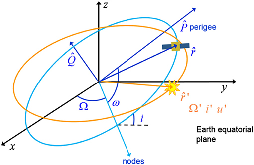
Figure 1. Geometry of the third body with respect to the spacecraft and the central body.

Note that the summation starts from k = 2 as the term zero of the series is influent as is a constant, while the term 1 simplifies with the second term of Equation (6). The average operation in eccentric anomaly, passing through the mean anomaly via dM = (1 − e cos E) dE can then be performed, assuming that the orbital elements of the spacecraft a, e, i, Ω, and ω are constant over one orbit revolution:

${\overline{F}}_k\left(A,B,e\right)=\frac{1}{2\pi }{\displaystyle \underset{-\pi }{\overset{\pi }{\int }}{F}_k\left(A,B,e,E\right)}\left(1-e\text{ cos }E\right)dE$

to obtain:

$\begin{array}{ll}\overline{R}\left(r,r^{\prime }\right)=\frac{{\mu }^{\prime }}{r^{\prime }}{\displaystyle \sum _{k=2}^{\infty }{\delta }^k{\overline{F}}_k\left(A,B,e\right)}& (8)\end{array}$

where the averaged terms ${\bar{F}}_k(A,B,e)$ are reported in Kaufman and Dasenbrock (1972) and in Appendix in a more compact form. Note that the term 2 of Equation (8) is the one given by Chao-Chun (2005). Equation (8) can be now inserted into the Lagrange equations by computing the partial derivatives with respect to the orbital elements, considering that the dependences of the terms in Equation (8) are: A (Ω, i, ω, Ω′, i′, ω′ + f′), B(Ω, i, ω, Ω′, i′, ω′ + f′), and ${\bar{R}}_k(A,B,e)$ (see Appendix for details).

$\begin{array}{l}\frac{\partial {\overline{F}}_k}{\partial \Omega }=\frac{\partial {\overline{F}}_k}{\partial A}\frac{\partial A}{\partial \Omega }+\frac{\partial {\overline{F}}_k}{\partial B}\frac{\partial B}{\partial \Omega }\\ \frac{\partial {\overline{F}}_k}{\partial i}=\frac{\partial {\overline{F}}_k}{\partial A}\frac{\partial A}{\partial i}+\frac{\partial {\overline{F}}_k}{\partial B}\frac{\partial B}{\partial i}\\ \frac{\partial {\overline{F}}_k}{\partial \omega }=\frac{\partial {\overline{F}}_k}{\partial A}\frac{\partial A}{\partial \omega }+\frac{\partial {\overline{F}}_k}{\partial B}\frac{\partial B}{\partial \omega }\\ \frac{\partial {\overline{F}}_k}{\partial a}=\frac{k}{a}{\overline{R}}_k\\ \frac{\partial {\overline{F}}_k}{\partial e}& (9)\end{array}$

The derivatives up to the 8^th order of the Taylor series are reported by Kaufman and Dasenbrock (1972); we report them in Appendix in a more concise form up to order 6^th.

Earth Zonal Harmonic Potential

The disturbing function of the zonal harmonic potential is expressed also in terms of classical orbital elements. The zonal harmonics were modeled up to order 6 considering also the $J_2^2$ term (Blitzer, 1970; Liu and Alford, 1980). We report here only the term associated with J₂ that is the one most important one for the application considered in this work. However, all the terms were retained in the orbit propagation.

${\overline{R}}_{J_2}=W\frac{n{a}^2}{6}\frac{3{\text{cos}}^{2}i-1}{{\left(1-e^2\right)}^{3/2}}$

where W is the oblateness parameter

$W=\frac{3}{2}{J}_2\frac{R_{\text{Earth}}^2}{a^2}n$

where J₂ = 1.083 · 10⁻³ denotes the second zonal harmonic coefficient and R_Earth is the mean radius of the Earth. $n=\sqrt{{\mu }_{\mathrm{\text{Earth}}}/a^3}$ is the orbit angular velocity of the spacecraft on its orbit, with μ_Earth the gravitational constant of the Earth.

Model Validation

The averaged dynamical model described in section Orbit Evolution With Single-Averaged Disturbing Potential was validated by comparison with the actual ephemerides of two artificial satellites in highly-elliptical orbit: INTEGRAL and XMM-Newton. The orbit of INTEGRAL was used in Colombo et al. (2014a) and validated against the ephemerides from the NASA-Horizon system. XMM-Newton orbit was propagated in the time span from 1999/12/15 to 2013/01/01 with the initial Keplerian elements on 1999/12/15 at 15:00 as: a = 67045 km, e = 0.7951, i = 0.67988 rad, Ω = 4.1192 rad, ω = 0.99259 rad, true anomaly f = 3.2299 rad, and radius of the perigee 13,737 km. Figure 2 shows the results of the validation with the actual ephemerides form ESA (2013) (blue line). Luni-solar and Earth zonal harmonics perturbations are included in this validation with PlanODyn (red line) (Colombo, 2016). The reference system used is inertial, centered at the Earth, on the Earth equator.

FIGURE 2

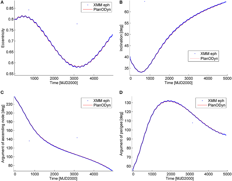
Figure 2. XMM Newton's ephemerides: actual ephemerides in blue and propagation with PlanODyn in red. (A) Eccentricity, (B) inclination, (C) argument of the ascending node, and (D) argument of the perigee. The x-axis represents the time in Modified Julian Date since 2000 (Time origin at 12:00 year 2000).

Orbit Evolution With Double-Averaged Disturbing Potential

Under the further assumption that the orbital elements do not change significantly during a full revolution of the perturbing body around the central body (i.e., Earth), the variation of the orbit over time can be approximately described through the disturbing potential double averaged over one orbit evolution of the s/c and over one orbital revolution of the perturbing body (either the Moon or the Sun) around the Earth. The terms of the disturbing potential due to the third body effect in Equation (3) can be substituted by the double-averaged one ${\overline{\stackrel{̄}{R}}}_{3-\mathrm{\text{Sun}}}$ and ${\overline{\stackrel{̄}{R}}}_{3-\mathrm{\text{Moon}}}$:

$\begin{array}{ll}\overline{\overline{R}}={\overline{R}}_{\text{zonal}}+{\overline{\overline{R}}}_{\text{3B-Sun}}+{\overline{\overline{R}}}_{\text{3B-Moon}}& (10)\end{array}$

$\begin{array}{ll}{\overline{\overline{R}}}_{\text{3B}}\left(r,r^{\prime }\right)=\frac{{\mu }^{\prime }}{r^{\prime }}{\displaystyle \sum _{k=2}^{\infty }{\delta }^k{\overline{\overline{F}}}_k\left(e,i,\Omega ,\omega ,i^{\prime }\right)}& (11)\end{array}$

In this work we decided to express the double-averaged potential with respect to the Keplerian elements described in the Earth's centered equatorial reference system. This will give a more complex expression for the potential in Equation (11), with respect to the one by El'yasberg (1967) and Costa and Prado (2000) but it has the advantage of avoiding the simplification that Moon and Sun orbit on the same plane and facilitating the introduction of the effect of the zonal harmonics.

The terms of the third body potential are obtained starting from the single-averaged terms, performing the averaging operation ${\overline{\stackrel{̄}{F}}}_k(A,B,e)$.

$\begin{array}{l}{\overline{\overline{F}}}_k\left(e,i,\Delta \Omega ,\omega ,i^{\prime }\right)=\frac{1}{2\pi }{\displaystyle {\int }_0^{2\pi }{\overline{F}}_k(A\left(\Omega ,i,\omega ,{\Omega }^{\prime },i^{\prime },{\omega }^{\prime }+f^{\prime }\right)},\\ B\left(\Omega ,i,\omega ,{\Omega }^{\prime },i^{\prime },{\omega }^{\prime }+f^{\prime }\right),e)d{f}^{\prime }\end{array}$

where ΔΩ = Ω − Ω′. The term up to order four of the potential were computed; only the second term ${\overline{\stackrel{̄}{F}}}_2$ is reported here as ${\overline{\stackrel{̄}{F}}}_3=0$:

$\begin{array}{l}{\overline{\overline{F}}}_2=\frac{1}{128}\cdot (\text{cos }\left(2i^{\prime }\right)\left(6+9e^2+90e^2\text{ cos }\left(2\omega \right){\sin }^{2}i\right)\\ +\left(2+3e^2\text{+}15e^2\text{ cos }\left(2\omega \right)\right)\left(1+6\text{ cos}\left(2\Delta \Omega \right){\sin }^2{i}^{\prime }\right)\\ +3\text{ cos }\left(2i\right)(\left(6+9e^2\right)\text{ cos }\left(2i^{\prime }\right)+\left(-2-3e^2+5e^2\text{ cos }\left(2\omega \right)\right)\\ \left(-1+2\text{ cos }\left(2\Delta \Omega \right){\sin }^2{i}^{\prime }\right))\\ 12\left(2+3e^2-5e^2\text{ cos }\left(2\omega \right)\right)\text{ cos }\left(2\Delta \Omega \right)\sin \left(2i\right)\sin \left(2i^{\prime }\right)\\ +120e^2\sin i\sin \left(2i^{\prime }\right)\sin \left(2\omega \right)\sin \left(\Delta \Omega \right)-\\ 120e^2\text{ cos }i{\sin }^2{i}^{\prime }sin\left(2\omega \right)\sin \left(2\Delta \Omega \right))& (12)\end{array}$

The evolution of the orbit in time can be then computed computing the partial derivatives of Equation (10) and substituting them into the Lagrange form of planetary equations Equations (1).

Note that, with the same procedure, the double averaged disturbing potential can be also written in the form proposed by El'yasberg (1967) and Costa and Prado (2000). A different reference system needs to be used, which is still centered at the central body (i.e., Earth) but the x-y plane lay on the perturbing body orbital plane, with its x-axis in the direction of the perturbing body on its orbit, the z-axis in the direction of the perturbing body angular momentum, and the y-axis that completes the reference system. The corresponding orbital elements are ${\alpha }_{\mathrm{\text{3Bsys}}}={\left[{\begin{array}{cccccc}{a}_{\mathrm{\text{3Bsys}}}& e_{\mathrm{\text{3Bsys}}}& i_{\mathrm{\text{3Bsys}}}& {\Omega }_{\mathrm{\text{3Bsys}}}& {\omega }_{\mathrm{\text{3Bsys}}}& M\\ \end{array}}_{\mathrm{\text{3Bsys}}}\right]}^T$. It is interesting to note that this rotating reference system is equivalent to the synodic system used in the circular restricted three-body problem.

In this case the eccentricity unit vector ${\widehat{\text{P}}}_{\mathrm{\text{3Bsys}}}$, the semilatus rectum unit vector ${\widehat{\text{Q}}}_{\mathrm{\text{3Bsys}}}$ and the unit vector to the third body $\widehat{\text{r}}{\prime }_{\mathrm{\text{3Bsys}}}$ have to be expressed with respect to the third body rotating system, through the following composition of rotations

$\begin{array}{l}{\widehat{P}}_{\text{3Bsys}}={\Re }_3\left({\Omega }_{\text{3Bsys}}\right){\Re }_1\left(i_{\text{3Bsys}}\right){\Re }_3\left({\omega }_{\text{3Bsys}}\right)\cdot {\left[\begin{array}{ccc}1& 0& 0\end{array}\right]}^T\\ {\widehat{R}}_{\text{3Bsys}}={\Re }_3\left({\Omega }_{\text{3Bsys}}\right){\Re }_1\left(i_{\text{3Bsys}}\right){\Re }_3\left({\omega }_{\text{3Bsys}}+\pi /2\right)\cdot {\left[\begin{array}{ccc}1& 0& 0\end{array}\right]}^T\\ {\widehat{r}}^{\prime }\text{3Bsys}={\Re }_3\left(0\right){\Re }_1\left(0\right){\Re }_3\left(0\right)\cdot {\left[\begin{array}{ccc}1& 0& 0\end{array}\right]}^T={\left[\begin{array}{ccc}1& 0& 0\end{array}\right]}^T& (13)\end{array}$

where ${\Omega }_{\mathrm{\text{3Bsys}}}={\Omega }_{\mathrm{\text{3Bsys}},0}-u^{\prime }$. By using Equations (13), the new expressions of A_3Bsys and B_3Bsys are found as

$\begin{array}{l}{A}_{\text{3Bsys}}={\widehat{P}}_{\text{3Bsys}}\cdot {{\widehat{r}}^{\prime }}_{\text{ 3Bsys}}\\ B_{\text{3Bsys}}={\widehat{Q}}_{\text{3Bsys}}\cdot {{\widehat{r}}^{\prime }}_{3\text{Bsys}}\end{array}$

that are function of $A_{\mathrm{\text{3Bsys}}}(u^{\prime }-{\Omega }_{\mathrm{\text{3Bsys}}},i_{\mathrm{\text{3Bsys}}},{\omega }_{\mathrm{\text{3Bsys}}})$, $B_{\mathrm{\text{3Bsys}}}(u^{\prime }-{\Omega }_{\mathrm{\text{3Bsys}}},i_{\mathrm{\text{3Bsys}}},{\omega }_{\mathrm{\text{3Bsys}}})$ so that the doubly averaged potential loses the dependence on the right ascension of the ascending node,

$\begin{array}{l}{\overline{\overline{F}}}_{\text{3Bsys},k}\left(e_{\text{3Bsys}},i_{\text{3Bsys}},{\omega }_{\text{3Bsys}}\right)\\ =\frac{1}{2\pi }{\displaystyle {\int }_0^{2\pi }{\overline{F}}_{\text{3Bsys},k}(A_{\text{3Bsys}}\left(u^{\prime }-{\Omega }_{\text{3Bsys}},i_{\text{3Bsys}},{\omega }_{\text{3Bsys}}\right),}\\ B_{\text{3Bsys}}\left(u^{\prime }-{\Omega }_{\text{3Bsys}},i_{\text{3Bsys}},{\omega }_{\text{3Bsys}}\right),e_{\text{3Bsys}})d{f}^{\prime }.\end{array}$

So equivalently to Equation (12), we can compute the terms 2 to 4 were we dropped the subscript 3BSys.

$\begin{array}{r}\hfill {\overline{\overline{F}}}_{\text{3Bsys},2}=\frac{1}{32}\left(\left(2+3e^2\right)\left(1+3\text{ cos}\left(2i\right)\right)+30e^2\text{ cos }\left(2\omega \right){\sin }^{2}i\right)\\ \hfill {\overline{\overline{F}}}_{\text{3Bsys},3}=0\\ \hfill {\overline{\overline{F}}}_{3Bsys,4}=\frac{9}{32768}(\left(8+40e^2+15e^4\right)\left(9+20\text{ cos }\left(2i\right)+35\text{ cos }\left(4i\right)\right)\\ \hfill +560e^2\left(2+e^2\right)\left(5+7\text{ cos }\left(2i\right)\right)\text{ cos }\left(2\omega \right){\sin }^{2}i\\ \hfill +5880e^4\text{ cos }\left(4\omega \right){\sin }^{4}i)\end{array}$

that are equivalent to the expression in El'yasberg (1967) and Costa and Prado (2000). If the partial derivatives of Equation (11) are inserted into the Lagrange form of planetary equations we get the expression of variation of elements double-averaged over one orbit evolution of the s/c and over one orbital revolution of the perturbing body (either the Moon or the Sun). Figure 3 compares the evolution of a high-altitude orbit using the single averaged dynamics (red line) and the double averaged dynamics (cyan line) in eccentricity and argument of the perigee with respect to the Moon plane. It is interesting to see the evolution in the phase space of eccentricity and argument of the perigee measured with respect to the Moon orbiting plane as done in Ely (2005) and Colombo et al. (2014a). For the initial conditions in Figure 3, the simplified model by El'yasberg (1967) and Kozai (1962) predicts a pure librational orbit (Ely, 2005) (magenta line) which, in reality, is corrupted by the coupling between Moon and Sun third-body effect and by the effect of J₂ (see the red and cyan lines). The double averaged propagation derived in Equation (12) is used for the Moon and the Sun in Equation (10) for obtaining the orbit propagation represented with the cyan line, while the single averaged propagation described in sections Luni-Solar Averaged Potential and Earth Zonal Harmonic Potential is used for obtaining the orbit propagation represented with the red line. The single and double average propagation are compared against the actual spacecraft ephemerides from the NASA Horizon system in blue. Both the single and the double averaged approach show very good accuracy against the real ephemerides. With respect to the pure librational loop predicted by the Lidov-Kozai dynamics, still a quasi-librational behavior can be noted and will be further studied in the next section through propagation via the single-averaged dynamics.

FIGURE 3

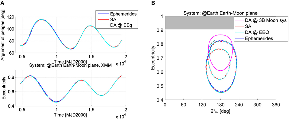
Figure 3. Evolution of a high altitude orbit under the effect of luni-solar and zonal perturbations. (A) Comparison of the actual ephemerides (blue) with single averaged (red) and double averaged (cyan) dynamics. (B) Evolution in the eccentricity-2ω phase space, where the argument of the perigee is measured with respect to the Moon plane.

Luni-Solar and Zonal Harmonics Maps

To the purpose of studying the long term evolution of many initial conditions, a grid was built in the domain of inclination, eccentricity and argument of the perigee. Equally spaced steps in initial eccentricity (19 steps between 0.05 and 0.9), initial inclination (20 steps between 0.5° and 90°) and initial right ascension of the ascending node (36 steps between 0° and 180°) were selected as starting points. Note that, inclination and argument of the perigee are here described with respect to the Moon plane reference system; in other words i is the inclination of the spacecraft orbit with respect to the Moon's orbit plane and ω is the argument of the perigee measured from the direction of the ascending node of the spacecraft's orbit with respect to the Moon's orbit plane. Each initial condition on the grid is propagated over 30 years with the tool PlanODyn (Colombo, 2016) using the single averaged dynamics. As mentioned before, only luni-solar and zonal harmonics perturbations are here taken into account as we want to analyze their interaction. For each initial condition we evaluate the change between the minimum and the maximum eccentricity that the spacecraft will attain during its motion (see Figure 4):

$\begin{array}{ll}\Delta e=e_{\max }-e_{\min }& (14)\end{array}$

with

$\begin{array}{l}{e}_{\max }=\underset{t}{\max }e\left(t\right)t\in \left[0\Delta t_{\text{disposal}}\right]\\ e_{\min }=\underset{t}{\min }e\left(t\right)t\in \left[0\Delta t_{\text{disposal}}\right]& (15)\end{array}$

setting Δt_disposal = 30years. As introduced the idea will be then to select limited Δe for graveyard disposal orbits or, at the opposite, maximum Δe orbits can be exploited for disposal through re-entry or for passive orbit transfer by exploiting the effects of perturbations.

FIGURE 4

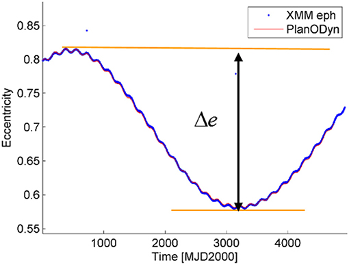
Figure 4. XMM-Newton orbit evolution and minimum and maximum eccentricity attained during the motion evolution. Blue line: actual ephemerides, red line: propagation with PlanODyn.

Figure 5 represents the result of the forward (a) and backward (b) integration for 30 years using, as initial conditions, the semi-major axis of XMM-Newton orbit, i.e., 67045.39 km, and different values of initial eccentricity and argument of the perigee in the grid, measured in the Moon reference system. The initial condition in terms of inclination and eccentricity corresponding to the one of the XMM-Newton orbit is represented by a star symbol. The maps are colored according to the maximum change of eccentricity Δe = e_max − e_min during the 30-year forward or backward propagation, respectively. If, for some initial conditions, the maximum eccentricity reaches the value of the critical eccentricity e_critical, corresponding to a perigee of h_{p, re-entry} = 50 km

$e_{\text{critical}}=1-\frac{R_E+h_{p,\text{ re-entry}}}{a}$

the integration is terminated and the corresponding initial condition is marked with a cross symbol in Figure 5. Note that, for those solutions, the actual orbit evolution should be computed considering the effect of aerodynamic drag. This was not done in the current work to limit the computational time, however, we expect that the effect of drag will act as a dumping of the dynamical system, decreasing the amplitude of the librational or rotational loops in the (e, 2ω) phase space and progressively decreasing the semi-major axis, as shown in Colombo and McInnes (2011) for the case of solar radiation pressure, Earth's oblateness and drag. This will be subject of future work.

FIGURE 5

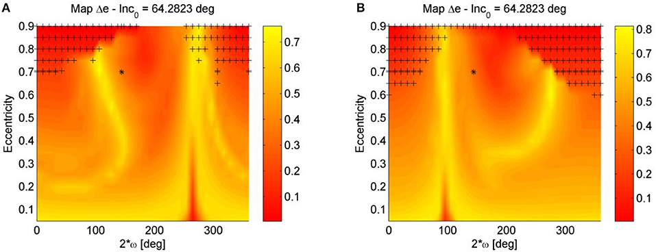
Figure 5. Luni-solar + zonal Δe maps for XMM Newton orbit: (A) Forward propagation, and (B) backward propagation. The initial inclination and the argument of the perigee are measured with respect to the Moon's plane.

Now, if we compute the maps considering both a forward and a backward propagation, both for 30 years, the map becomes more symmetric, as no particular choice (in terms of symmetry in the position of the Sun and the Moon) was made for the initial epoch. This is due to the fact that, if in the propagation the eccentricity reaches the maximum value e_impact corresponding to a perigee equal to the Earth radius,

$e_{\text{impact}}=1-\frac{R_E}{a}$

the integration is terminated. Performing, from each starting point in the grid both a forward and a backward integration in time, instead, allows characterizing the dynamics in the phase space (e, 2ω) in terms of reachable conditions. Figure 6A shows the forward-backward maps starting from a semi-major axis of 67045.39 km, where now Δe = e_max − e_min is computed as

$\begin{array}{l}{e}_{\max }=\underset{t}{\max }e\left(t\right)t\in \left[-\Delta t_{\text{disposal}}+\Delta t_{\text{disposal}}\right]\\ e_{\min }=\underset{t}{\min }e\left(t\right)t\in \left[-\Delta t_{\text{disposal}}+\Delta t_{\text{disposal}}\right]\end{array}$

setting Δt_disposal = 30years. The map in Figure 6A present and island of low eccentricity variation close to the initial condition of XMM Newton's orbit. The condition of quasi-frozen orbit is located around 2ω₀ = 180deg and e₀ ≃ 0.8. The solutions around this conditions librate around the limited-eccentricity orbit. Other two islands of small eccentricity are present in this map, one around 2ω₀ = 180deg and e₀ ≃ 0.2 and another around 2ω₀ = 0deg and high values of the initial eccentricities. Those solution corresponds to orbits which rotate is terms of ω but have a limited variation in terms of eccentricity. Solutions starting at eccentricity close to zero have the highest variation of eccentricity. This means that for this semi-major axis and inclination, spacecraft on circular orbit can naturally get on an elliptical orbit and eventually reach re-entry.

FIGURE 6

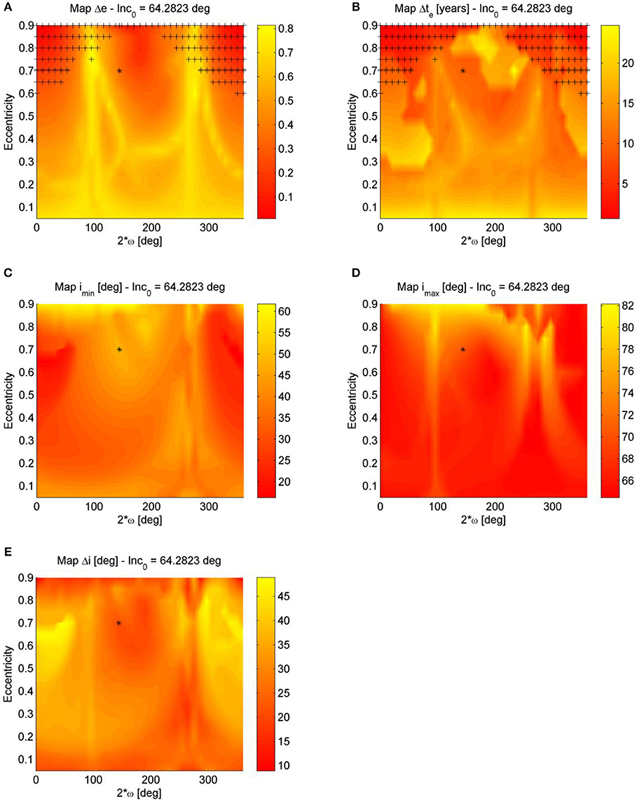
Figure 6. Luni-solar + zonal maps for semi-major axis of XMM Newton orbit a = 67045.39 km: (A) Δe map, (B) Δt_e map, (C) i_min map, (D) i_max map, and (E) Δi map. The initial inclination and the argument of the perigee are measured with respect to the Moon's plane.

In order to approximate the half-period of the oscillation in the (e, 2ω) phase space, the time interval between the points when the spacecraft attain the minimum and the maximum eccentricity is computed (as an averaged between the forward and the backward propagation) and shown in Figure 6B. From Figure 6B it is for example possible to see that the quasi-frozen solution is stable for 30 years. Indeed, due to the oscillation in inclinations, which has longer period, the orbit may encounter some instability is a longer propagation time is chosen as the eccentricity may increase beyond the critical eccentricity [this can be noted for example in the case of the INTEGRAL spacecraft (Colombo et al., 2014a)]. The maximum and minimum inclination attained with respect to the Moon's plane are shown in Figures 6C, D, while the variation of inclination is represented in Figure 6E. As it can be seen from Figure 6E the limited eccentricity conditions do not have a zero variation of the inclination; therefore, the long-term stability over longer time period is not guaranteed and an analysis over longer timeframe is required.

Once the behavior on the (e, 2ω) phase space is understood by looking at the map showing the result of the backward and forward propagation as in Figure 6A, it is possible to study the sensitivity to the initial condition in inclination with respect to the Moon's plane. In Figure 7, the Δe maps are computed for different starting inclination with respect to the orbiting plane of the Moon to show how the phase space changes depending on the initial inclination. For low inclinations the solutions are all rotational in ω (measured with respect to the Moon's plane) and exhibits a higher variation of eccentricity the more the initial eccentricity is high (Figures 7A–E) and for a high initial eccentricity the solutions which exhibits a higher eccentricity variation are characterized by 2ω₀ = 180deg. This behavior is clearer in Figures 7F–L: the solutions initiating from the yellow area of high initial eccentricities and 2ω₀ = 180deg rotate in ω, while quasi-equilibrium solutions exists at high eccentricities and 2ω₀ ≃ 0 deg (red island around 2ω₀ ≃ 0 deg). This is also visible from Figure 8 that shows the orbit evolution in the (e, 2ω) phase space for many initial conditions all at starting inclination with respect to the Moon's plane of 45° and semi-major axis equal to 67045.39 km but for different starting ω₀ (color code) and for different initial eccentricity (Figures 9A,L).

FIGURE 7

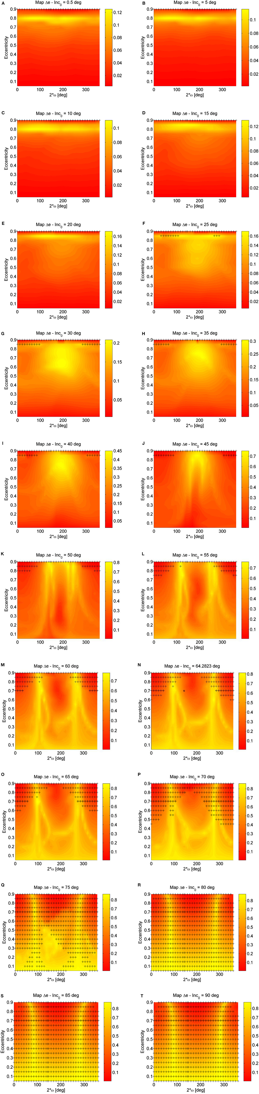
Figure 7. Luni-solar + zonal Δe maps for semi-major axis equal to 67045.39 km (XMM Newton's orbit) for different values of initial inclination with respect to the orbiting plane of the Moon. The initial inclination and the argument of the perigee are measured with respect to the Moon's plane. (A) Initial inclination = 0.5 deg. (B) Initial inclination = 5 deg. (C) Initial inclination = 10 deg. (D) Initial inclination = 15 deg. (E) Initial inclination = 20 deg. (F) Initial inclination = 25 deg. (G) Initial inclination = 30 deg. (H) Initial inclination = 35 deg. (I) Initial inclination = 40 deg. (J) Initial inclination = 45 deg. (K) Initial inclination = 50 deg. (L) Initial inclination = 55 deg. (M) Initial inclination = 60 deg. (N) Initial inclination = 64.2823 deg. (O) Initial inclination = 65 deg. (P) Initial inclination = 70 deg. (Q) Initial inclination = 75 deg. (R) Initial inclination = 80 deg. (S) Initial inclination = 85 deg. (T) Initial inclination = 90 deg.

FIGURE 8

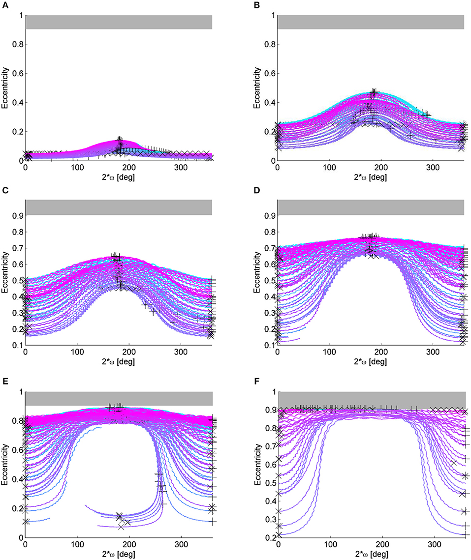
Figure 8. Maps for initial inclination with respect to the Moon's plane of 45° and semi-major axis equal to 67045.39 km. The initial inclination and the argument of the perigee are measured with respect to the Moon's plane. (A) Eccentricity-2ω plot for e₀ = 0.05. (B) Eccentricity-2ω plot for e₀ = 0.25. (C) Eccentricity-2ω plot for e₀ = 0.45. (D) Eccentricity-2ω plot for e₀ = 0.65. (E) Eccentricity-2ω plot for e₀ = 0.8. (F) Eccentricity-2ω plot for e₀ = 0.9.

FIGURE 9

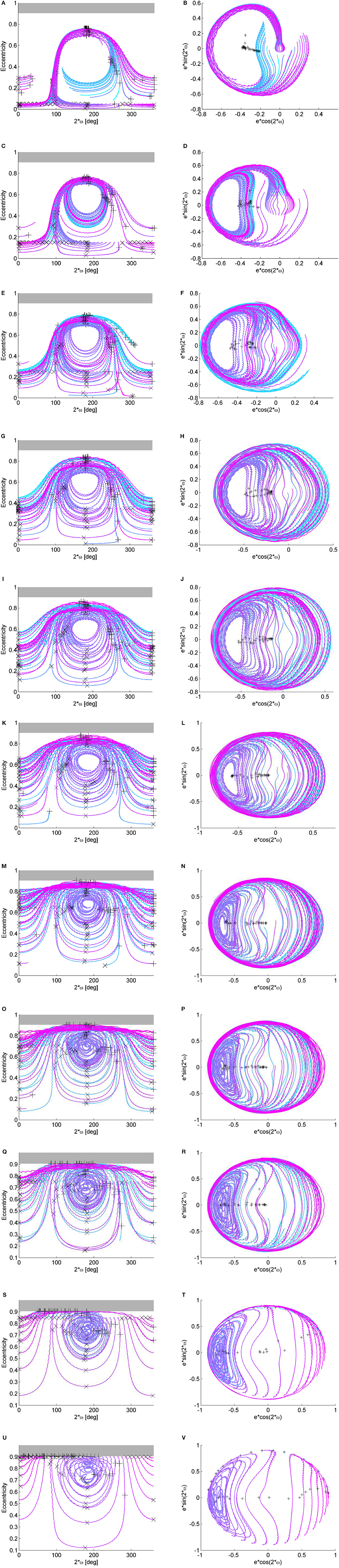
Figure 9. Maps for initial inclination with respect to the Moon's plane of 64.28° and semi-major axis equal to 67045.39 km. The initial inclination and the argument of the perigee are measured with respect to the Moon plane. (A) Eccentricity-2ω plot: e₀ = 0.05. (B) Polar plot: e₀ = 0.05. (C) Eccentricity-2ω plot: e₀ = 0.15. (D) Polar plot: e₀ = 0.15. (E) Eccentricity-2ω plot: e₀ = 0.25. (F) Polar plot: e₀ = 0.25. (G) Eccentricity-2ω plot: e₀ = 0.35. (H) Polar plot: e₀ = 0.35. (I) Eccentricity-2ω plot: e₀ = 0.45. (J) Polar plot: e₀ = 0.45. (K) Eccentricity-2ω plot: e₀ = 0.55. (L) Polar plot: e₀ = 0.55. (M) Eccentricity-2ω plot: e₀ = 0.65. (N) Polar plot: e₀ = 0.65. (O) Eccentricity-2ω plot: e₀ = 0.705. (P) Polar plot: e₀ = 0.705. (Q) Eccentricity-2ω plot: e₀ = 0.75. (R) Polar plot: e₀ = 0.75. (S) Eccentricity-2ω plot: e₀ = 0.85. (T) Polar plot: e₀ = 0.85. (U) Eccentricity-2ω plot: e₀ = 0.90. (V) Polar plot: e₀ = 0.90.

Going back at the Δe maps in Figure 7, a new island appear for inclinations above 45° at low eccentricities and 2ω₀ ≃ 180 deg of quasi-equilibrium solutions and librational solutions (Figure 7L), while the island at high eccentricities and 2ω₀ ≃ 0 deg move up. This is clearly visible from Figure 9 that shows the orbit evolution in the (e, 2ω) phase space and the polar plots for many initial conditions all at starting inclination with respect to the Moon's plane of 64.28° and semi-major axis equal to 67045.39 km but for different starting ω₀ (color code) and for different initial eccentricity (Figures 9A, L).

For the semi-major axis considered (67045.39 km) i₀ = 45deg is approximately the critical inclination (Kozai, 1962; Costa and Prado, 2000). Indeed, for inclination higher than the critical values, circular orbits get very elliptic (see yellow path in Figures 7L–T). The more the initial inclination with respect to the Moon increases, the more the initial orbit reaches the critical eccentricity for re-entry (cross symbols). Finally, for initial inclinations above i₀ = 70 deg, the quasi-equilibrium solutions in correspondence of 2ω₀ ≃ 180 deg are in correspondence of e₀ > e_critic, therefore not feasible, however, the fast eccentricity solution starting from e₀ = 0 still exist. It is important to remember that, even if qualitatively similar, the behavior depends also on the orbit semi-major axis that here is kept constant.

Re-entry or Graveyard Design

The initial conditions characterized by limited Δe variation identified in Figures 7L–T could be selected as graveyard orbits (Ely, 2005), while the high eccentricity variation solutions as initial condition for passive eccentricity increase to target Earth re-entry. It must be stressed that, while a re-entry trajectory will remove completely the spacecraft from the space environment, a graveyard solution will leave the satellite on a long-term stable orbit. In this sense, however, the time within which the orbit stability has been verified becomes an important parameter as the orbit may de-stabilize afterwards (Daquin et al., 2016). On the other side, it must be noted that re-entry need to be carefully designed according to casualty risk constraints on ground (Merz et al., 2015).

This section will exploit the findings from the previous Sections to design the end-of-life disposal for XMM-Newton mission by enhancing the effect of the natural dynamics or luni-solar and J₂ perturbation. The approach for the optimal Δv computation was detailed in Colombo et al. (2014a) where the re-entry of the INTEGRAL spacecraft was designed. The approach is summarized here and extended to the graveyard disposal design. For the disposal a single maneuver is considered, performed during the natural orbit evolution of the spacecraft (computed under the effect of perturbations). The finite variation in orbital elements Δα achieved by an impulsive maneuver, is computed through Gauss' planetary equations written in finite-difference form and the new set of orbital elements after the maneuver is propagated with PlanODyn (Colombo, 2016) in single-averaged orbital elements considering luni-solar perturbation and the zonal terms of the Earth gravity potential for the maxim disposal time Δt_disposal = 30 years. Re-entry transfer orbits are selected that achieve in the propagation time Δt_disposal the critical eccentricity e_critical as in Colombo et al. (2014a), while for selecting a suitable graveyard disposal, solutions that attain the minimum Δe over the propagation time are selected. A graveyard orbit is designed imposing that after the maneuver, the variation of the eccentricity in time stays limited, that is Δe in Equation (14) is minimized. In order to analyze a wide range of disposal dates, different starting dates for the disposal were selected, whereas, to determine the maneuver magnitude Δv and direction (α and β) and the point on the orbit where the maneuver is performed f, an optimization procedure with genetic algorithm was performed in order to find the optimal set of parameters x = [Δv α β f] that minimizes the cost function J = Δe + w · Δv where w is a weighting factor set equal to 1,000. Rather than optimizing the timing for the optimal disposal maneuver; it was chosen instead to leave the time for that maneuver as a parameter of a sensitivity analysis; in other words, the insertion to graveyard was optimized for many different starting dates to analyze how the natural evolution of the orbit can be exploited. A maximum magnitude for the Δv is considered based on the available on-board propellant.

XMM-Newton Re-entry Disposal

The time interval considered for the disposal design is from 2013/01/01 to 2035/01/01. The maximum Δv available for the maneuver sequences is estimated to be 40.5 m/s in 2013/01/01 (Colombo et al., 2014a). The re-entry can be considered satisfied when an altitude of 50 km or lower is reached from the Earth's surface. The natural orbit evolution of the spacecraft is shown in Figure 10 in the (e, 2ω) phase space. The black points represent the initial conditions (and corresponding starting time) considered for the maneuver of disposal. For each starting point an impulsive maneuver of maximum magnitude equal to two times the available Δv on board on 2013/01/01 (equal to 81.1 m/s) is optimized in direction in order to maximize the following variation of the orbit eccentricity in the available Δt_disposal. The results of the Δv optimization for each initial starting condition along the natural orbit evolution are reported in Figure 10 in colored line. Moving toward the external part of the phase space correspond to target the yellow regions in Figure 7P (for that map the initial semi-major axis and inclination are the one of the XMM spacecraft). Corresponding to large eccentricity variation. However, as it can be seen from Figure 10B, re-entry is not achievable within the considered Δt_disposal for the maximum Δv considered (equal to 81.1 m/s) as the minimum perigee reached (among all the possible starting dates) is equal or above 4,700 km (too high for re-entry). This demonstrates that re-entry for XMM-Newton is not a feasible option during this time range as the propellant requirements for such a disposal would be over the actual propellant on-board the spacecraft. Figure 10A represents the maneuver in the eccentricity-perigee angle (measured with respect to the Earth-Moon plane) phase space. Future studies for XMM-Newton disposal through re-entry could investigate the possibility to increase the propagation time to verify whether the interaction between Moon and Sun third body perturbation will cause a natural decrease in the perigee. However, it needs to be taken into account that the available Δv on-board the spacecraft decreases with time due to orbit correction.

FIGURE 10

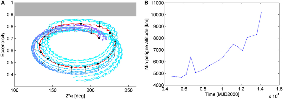
Figure 10. XMM-Newton re-entry disposal. (A) Maneuvers in the eccentricity-2ω phase space (black points: starting times analyzed for the re-entry disposal). (B) Minimum perigee reached during the orbit long-term evolution for each solution. The initial inclination and the argument of the perigee are measured with respect to the Moon's plane.

XMM-Newton Graveyard Disposal

Another disposal option that can be investigated for HEO in case the re-entry option is not feasible, is the option to transfer the spacecraft into a graveyard orbit. The existence of long-term stable orbits can be investigated, where the evolution of the orbital elements due to natural perturbation is limited. Such orbits can be chosen as graveyard orbits. Such orbits are visible in the map in Figure 7P (for that map the initial semi-major axis and inclination are the one of the XMM spacecraft) with a red color corresponding to a small variation of eccentricity. Importantly, note that the strategy would ideally aims at reaching the center of libration in the phase space; however, due to the limitation in the maximum available Δv, imposed as an upper bound for the global optimization, a more stable orbit cannot be reached, but only an orbit that is more stable than the nominal one. In other words, optimal solution is to move toward the center of the phase space loop. Also note that, due to the chaotic behavior of the orbit evolution under the effect of luni-solar perturbation, a driving factor is the time period Δt_graveyard used for the propagation of the orbit after the maneuver to compute Equations (15) and (14). For this study Δt_graveyard was set equal to 30 years, but this number can be easily increased for further work. Figure 11A shows the optimal maneuver for a transfer into a graveyard orbit for each starting time analyzed. The maneuver is represented in the phase space of eccentricity, inclination and anomaly of the percenter with respect to the Earth-Moon plane. The magnitude of the maneuver is always close to the upper bound of available Δv as is clear that a higher Δv would allow reaching a more stable orbit. However, the new graveyard orbit reduces at least the oscillations in eccentricity, preventing the spacecraft from an uncontrolled re-entry within the 30-year period. As an example, a disposal trajectory, whose maneuver is performed on 20/04/2016, is shown in Figure 11B.

FIGURE 11

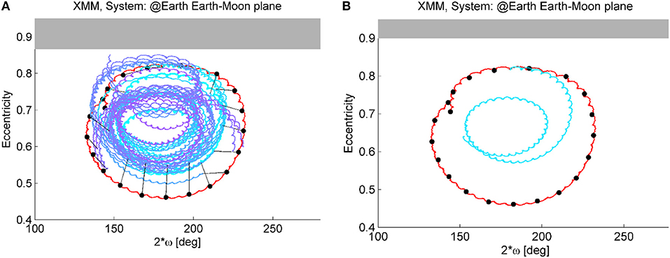
Figure 11. XMM-Newton graveyard disposal. (A) Optimal maneuvers in the eccentricity-2ω phase space (black points: starting times analyzed for the re-entry disposal). (B) Example of a disposal trajectory (cyan line). The initial inclination and the argument of the perigee are measured with respect to the Moon's plane.

Conclusion

This article analyzed the effect of luni-solar perturbations and the Earth's oblateness on the stability of highly elliptical orbits. The disturbing potential of the third body perturbation is written in Taylor expansion of the distances to the third body. The potential is firstly averaged over the revolution of the spacecraft around the Earth (mean anomaly) then is averaged again over the revolution of the perturbing body around the Earth. The existence of quasi-frozen, librational and rotational trajectories foreseen by the Kozai's analytical theory are found also when the Sun third body effect and the Earth's oblateness are included in the simulation. Maps are constructed over a wide domain of initial conditions in terms of eccentricity, inclination and argument of the perigee with respect to the Moon's plane. These maps represents the change in eccentricity over a long time space and in general can be used to study the orbit stability properties. These findings are finally used to design the end-of-life disposal for the XMM-Newton spacecraft as graveyard orbit injection or Earth re-entry. In this work, the effect of tesseral harmonics was not taken into account, while this could be important for creating maps in correspondence of lower semi-major axis, for example for Geostationary transfer orbits; the same approach however could be followed.

Data Availability

The datasets generated for this study can be found in the repository at the link www.compass.polimi.it/publications (Colombo, 2018).

Author Contributions

CC contributed to the conception and design of the study by writing the PlanODyn code and simulating the maps contained in this paper. She wrote the first draft of the manuscript firstly presented at the 25th AAS/AIAA Space Flight Mechanics Meeting, in Williamsburg (VA) in January 2015.

Funding

CC acknowledges the support received by the Marie Curie grant 302270 (SpaceDebECM - Space Debris Evolution, Collision risk, and Mitigation) and the European Research Council (ERC) under the European Union's Horizon 2020 research and innovation programme (grant agreement No 679086 - COMPASS). These two projects brought to the development and completion of this work.

Conflict of Interest Statement

The author declares that the research was conducted in the absence of any commercial or financial relationships that could be construed as a potential conflict of interest.

Acknowledgments

This work was initiated as a follow-up of a study for the European Space Agency named End-Of-Life Disposal Concepts for Lagrange-Point and Highly Elliptical Orbit Missions (Contract No. 4000107624/13/F/MOS). The author would like to acknowledge the team members of the ESA study: F. Letizia, S. Soldini, H. Lewis, E. M. Alessi, A. Rossi, L. Dimare, M. Vasile, M. Vetrisano, Van der Weg W., and M. Landgraf.

References

Alessi, E. M., Deleflie, F., Rosengren, A. J., Rossi, A., Valsecchi, G. B., Daquin, J., et al. (2016). A numerical investigation on the eccentricity growth of gnss disposal orbits. Celest. Mech. Dynam. Astron. 125, 71–90. doi: 10.1007/s10569-016-9673-4

CrossRef Full Text | Google Scholar

Alessi, E. M., Schettino, G., Rossi, A., and Valsecchi, G. B. (2018). Natural highways for end-of-life solutions in the leo region. Celest. Mech. Dynam. Astron. 130:34. doi: 10.1007/s10569-018-9822-z

CrossRef Full Text | Google Scholar

Armellin, R., Di Mauro, G., Rasotto, M., Madakashira, H. K., Lara, M., and San-Juan, J. F. (2014). End-of-Life Disposal Concepts for Lagrange-Points and HEO Missions. Final Report, ESA/ESOC contract No. 4000107624/13/F/MOS.

Battin, R. H. (1999). An Introduction to the Mathematics and Methods of Astrodynamics. Reston: Aiaa Educational Series.

Google Scholar

Blitzer, L. (1970). Handbook of Orbital Perturbations. Tucson, AZ: University of Arizona.

Cefola, P. J., and Broucke, R. (1975). “On the formulation of the gravitational potential in terms of equinoctial variables,” in 13th Aerospace Sciences Meeting (Pasadena, CA: American Institute of Aeronautics and Astronautics). doi: 10.2514/6.1975-9

CrossRef Full Text | Google Scholar

Chao-Chun, G. C. (2005). Applied Orbit Perturbation and Maintenance. El Segundo, CA.

Google Scholar

Colombo, C. (2015). “Long-term evolution of highly-elliptical orbits: luni-solar perturbation effects for stability and re-entry,” in Proceedings of the 25th AAS/AIAA Space Flight Mechanics Meeting (Williamsburg: AAS-15–395).

Colombo, C. (2016). “Planetary orbital dynamics (Planodyn) suite for long term propagation in perturbed environment,”. Proceedings of the 6th International Conference on Astrodynamics Tools and Techniques (ICATT) (Darmstadt: ESOC/ESA).

Google Scholar

Colombo, C. (2018). Long-Term Evolution of Highly-Elliptical Orbits: Luni-Solar Perturbation Effects for Stability and Re-Entry. COMPASS. Grant agreement 679086. Politecnico di Milano. Available online at: www.compass.polimi.it/publications (accessed August 5, 2018).

Google Scholar

Colombo, C., and Gkolias, I. (2017). “Analysis of the orbit stability in the geosyncronous region for end-of-life disposal,”in Proceedings of the 7th European Conference on Space Debris (Darmstadt: ESA/ESOC).

Colombo, C., Letizia, F., Alessi, E. M., and Landgraf, M. (2014a). “End-of-life earth re-entry for highly elliptical orbits: the integral mission,” in Proceedings of the 24th AAS/AIAA Space Flight Mechanics Meeting (Santa Fe: AAS 14-325).

Google Scholar

Colombo, C., Letizia, F., Soldini, S., Lewis, H., Alessi, E. M., Rossi, A., et al. (2014b). End-of-Life Disposal Concepts for Lagrange-Point and Highly Elliptical Orbit Missions. Final Report, ESA/ESOC contract No. 4000107624/13/F/MOS.

Google Scholar

Colombo, C., and McInnes, C. (2011). Orbital dynamics of “Smart-Dust” devices with solar radiation pressure and drag. J. Guid. Control Dyn. 34, 1613–1631. doi: 10.2514/1.52140

CrossRef Full Text | Google Scholar

Cook, G. E. (1962). Luni-solar perturbations of the orbit of an earth satellite. Geophy. J. Int. 6, 271–291.

Google Scholar

Costa, I. V. d., and Prado, A. F. B. d. A. (2000). Orbital evolution of a satellite perturbed by a third body. Adv. Space Dyn.

Google Scholar

Daquin, J., Rosengren, A. J., Alessi, E. M., Deleflie, F., Valsecchi, G. B., and Rossi, A. (2016). The dynamical structure of the meo region: long-term stability, chaos, and transport. Celest. Mech. Dynam. Astron. 124, 335–366. doi: 10.1007/s10569-015-9665-9

CrossRef Full Text | Google Scholar

Draim, J. E., Inciardi, R., Proulx, R., Cefola, P. J., Carter, D., and Larsen, D. E. (2002), Beyond geo—using elliptical orbit constellations to multiply the space real estate. Acta Astronaut. 51, 467–489. doi: 10.1016/s0094-5765(02)00036-x

CrossRef Full Text | Google Scholar

Ely, T. A. (2005). Stable constellations of frozen elliptical inclined lunar orbits. J. Astronaut. Sci. 3, 301–16.

Ely, T. A. (2014). Mean element propagations using numerical averaging. J. Astron. Sci. 61, 1–30. doi: 10.1007/s40295-014-0020-2

CrossRef Full Text | Google Scholar

El'yasberg, P. E. (1967). Introduction to the Theory of Flight of Artificial Earth Satellites. (Translated from Russian). NASA.

ESA (2013). Xmm-Newton Users Handbook. European Space Agency.

Gkolias, I., and Colombo, C. (2017). “End-of-life disposal of geosynchronous satellites,” in Proceedings of the 68th International Astronautical Congress (Adelaide: IAC-17-A6.4.3).

Google Scholar

Gkolias, I., Daquin, J., Gachet, F., and Rosengren, A. J. (2016). From order to chaos in earth satellite orbits. Astron. J. 152:119. doi: 10.3847/0004-6256/152/5/119

CrossRef Full Text | Google Scholar

Jenkin, A. B., and McVey, J. (2008). “Lifetime reduction for highly inclined, highly eccentric disposal orbits by changing inclination,” in Proceedings of the AIAA/AAS Astrodynamics Specialist Conference and Exhibit (Hawaii: AIAA/AAS Honolulu).

Google Scholar

Katz, B., Dong, S., and Malhotra, R. (2011). Long-term cycling of kozai-lidov cycles: extreme eccentricities and inclinations excited by a distant eccentric perturber. Phy. Rev. Lett. 107:181101. doi: 10.1103/PhysRevLett.107.181101

PubMed Abstract | CrossRef Full Text | Google Scholar

Kaufman, B., and Dasenbrock, R. (1972). Higher Order Theory for Long-Term Behaviour of Earth and Lunar Orbiters. NRL Repot 7527. Naval Research Laboratory.

Kozai, Y. (1962). Secular perturbations of asteroids with high inclination and eccentricity. Astron. J. 67, 591–598. doi: 10.1086/108790

CrossRef Full Text | Google Scholar

Krivov, A. V., and Getino, J. (1997). Orbital evolution of high-altitude balloon satellites. Astron. Astrophys. 318, 308–314.

Google Scholar

Lara, M., San-Juan, J., López, L., and Cefola, P. (2012). On the third-body perturbations of high-altitude orbits. Celest. Mechan. Dynam. Astron. 113, 435–452. doi: 10.1007/s10569-012-9433-z

CrossRef Full Text | Google Scholar

Laskar, J., and Bou,é, G. (2010). Explicit expansion of the three-body disturbing function for arbitrary eccentricities and inclinations. A&A 522:A60.

Google Scholar

Lidov, M. L. (1962). The evolution of orbits of artificial satellites of planets under the action of gravitational perturbations of external bodies. Planet. Space Sci. 9, 719–759. doi: 10.1016/0032-0633(62)90129-0

CrossRef Full Text | Google Scholar

Liu, J. J. F., and Alford, R. L. (1980). Semianalytic theory for a close-earth artificial satellite. J. Guid. Control Dyn. 3, 304–311.

Google Scholar

Merz, K., Krag, H., Lemmens, S., Funke, Q., Böttger, S., Sieg, D., et al. (2015). “Orbit aspects of end-of-life disposal from highly eccentric orbits,” in Proceedings of the 25th International Symposium on Space Flight Dynamics ISSFD (Munich).

Murray, C. D., and Dermott, S. F. (1999). Solar System Dynamics. Cambridge University Press. doi: 10.1017/CBO9781139174817

CrossRef Full Text | Google Scholar

Naoz, S., Farr, W. M., Lithwick, Y., Rasio, F. A., and Teyssandier, J. (2013). Secular dynamics in hierarchical three-body systems. Month. Notices. R. Astron. Soc. 431, 2155–2171. 10.1093mnrasstt302

Google Scholar

Rossi, A., Alessi, E. M., Valsecchi, G. B., Lewis, H. G., Colombo, C., Anselmo, L., et al. (2015). Disposal Strategies Analysis for Meo Orbits. ESA contract 4000107201/12/F/MOS.

Shapiro, E. B. (1995). Phase plane analysis and observed frozen orbit for the topex/poseidon mission. Adv. Astron. Sci. 91, 853–872.

Google Scholar

Skoulidou, D. K., Rosengren, A. J., Tsiganis, K., and Voyatzis, G. (2017). “Cartographic study of the meo phase space for passive debris removal,” in 7th European Conference on Space Debris (Darmstadt).

Google Scholar

Srongprapa, P. (2015). Mapping the Effects of Earth's Gravity Field on the Orbit Propagation of Gto Spacecraft a Study within the Context of Passive De-Orbiting through the Use of Perturbations. Faculty of Engineering and the Environment, University of Southampton, Southampton.

Google Scholar

Appendix

Luni-Solar Perturbation Development

The average disturbing potential due to the third body effect can be written as Kaufman and Dasenbrock (1972):

$\begin{array}{ll}\overline{R}\left(r,r^{\prime }\right)=\frac{{\mu }^{\prime }}{r^{\prime }}{\displaystyle \sum _{k=2}^{\infty }{\delta }^k{\overline{F}}_k\left(A,B,e\right)}& (16)\end{array}$

where μ′ is the gravitational coefficient of the third body, r′ is the spacecraft distance to the third body. The factors of the Taylor expansion can be written as function of the power of the ratio between the orbit semi-major axis and the distance to the third body δ = a/r′ multiplied by the function ${\overline{R}}_k(A,B,e)$, which is function of the orbit eccentricity and the function A and B (Chao-Chun, 2005) that are here written in terms of A_Blizer and B_Blizer given by Blitzer (1970) to show the link between them.

$\begin{array}{l}A=\text{cos }\omega A_{\text{Blizer}}+\sin \omega A_{\text{Blizer}}\\ B=-\sin \omega A_{\text{Blizer}}+\text{cos }\omega A_{\text{Blizer}}\\ A_{\text{Blizer}}=\text{cos }\Delta \Omega \text{ cos }{u}^{\prime }+\text{cos }{i}^{\prime }\sin u^{\prime }\sin \Delta \Omega \\ B_{\text{Blizer}}=-\text{cos }i\left(\text{cos }{u}^{\prime }\sin \Delta \Omega -\text{cos }{i}^{\prime }\text{ cos }\Delta \Omega \sin u^{\prime }\right)\\ +\sin i\sin i^{\prime }\sin u^{\prime }\end{array}$

The terms ${\overline{F}}_k(A,B,e)$ in Equation (16) are given by Kaufman and Dasenbrock (1972) and are here reported in a more compact form up to order 6th as:

${\overline{F}}_2\left(A,B,e\right)=\frac{1}{4}\left(\left(-2+3A^2+3B^2\right)-3\left(1-4A^2+B^2\right)e^2\right)$

${\overline{F}}_3\left(A,B,e\right)=\frac{5}{16}Ae\left(\left(12-15A^2-15B^2\right)+\left(9-20A^2+15B^2\right)e^2\right)$

$\begin{array}{l}{\overline{F}}_4\left(A,B,e\right)=\frac{3}{64}(\left(8-40A^2+35A^4-40B^2+70A^2{B}^2+35B^4\right)\\ +\left(40-410A^2+420A^4+10B^2+350A^2{B}^2-70B^4\right)e^2\\ +\left(15-180A^2+280A^4+30B^2-420A^2{B}^2+35B^4\right)e^4)\end{array}$

$\begin{array}{l}{\overline{F}}_5\left(A,B,e\right)=-\frac{21}{128}Ae((40-140A^2+105A^4-140B^2\\ +210A^2{B}^2+105B^4)(100-490A^2\\ +420A^4+70B^2+210A^2{B}^2-210B^4)e^2\\ +(25-140A^2+168A^4+70B^2-420A^2{B}^2\\ +105B^4)e^4)\end{array}$

$\begin{array}{l}{\overline{F}}_6\left(A,B,e\right)=\frac{1}{256}((-80+840A^2-1890A^4+1155A^6\\ +840B^2-3780A^2{B}^2+3465A^4{B}^2-1890B^4\\ +3465A^2{B}^4+1155B^6)\\ +(-840+16380A^2\\ -42525A^{4}27720A^6+1260B^2-39690A^2{B}^2\\ +51975A^4{B}^2+2835B^4+20790A^2{B}^4\\ -3465B^6+20790A^2{B}^4-3465B^6)e^2\\ +(-1050+23625A^2-75600A^4+55440A^6\\ -1575B^2+28350A^2{B}^2-51975A^2{B}^4\\ +3465B^6)e^4\\ +(-175+4200A^2-15120A^4\\ +14784A^6-525B^2+15120A^2{B}^2-55440A^4{B}^2\\ -945B^4+27720A^2{B}^4-1155B^6)e^6)\end{array}$

The derivatives of Equation (16) with respect to the orbital elements need to be computed to be inserted into the Lagrange planetary equations Equation (4) as in Equation (9), with

$\begin{array}{l}\frac{\partial B}{\partial \Omega }=\text{cos }\omega \left(-\text{cos }{u}^{\prime }\sin \Delta \Omega +\text{cos }{i}^{\prime }\text{ cos }\Delta \Omega \sin u^{\prime }\right)\\ -\text{cos }i\sin \omega \left(\text{cos }\Delta \Omega \text{ cos }{u}^{\prime }+\text{cos }{i}^{\prime }\sin \Delta \Omega \sin u^{\prime }\right)\end{array}$

$\begin{array}{l}\frac{\partial B}{\partial \Omega }=\sin \omega \left(\text{cos }{u}^{\prime }\sin \Delta \Omega -\text{cos }{i}^{\prime }\text{ cos }\Delta \Omega \sin u^{\prime }\right)\\ -\text{cos }i\text{ cos }\omega \left(\text{cos }\Delta \Omega \text{ cos }{u}^{\prime }+\text{cos }{i}^{\prime }\sin \Delta \Omega \sin u^{\prime }\right)\end{array}$

$\frac{\partial A}{\partial i}=C_{\text{Blitzer}}\sin \omega$

$\frac{\partial B}{\partial i}=C_{\text{Blitzer}}\text{ cos }\omega$

$\frac{\partial A}{\partial \omega }=B$

$\frac{\partial B}{\partial \omega }=-A$

where (Blitzer, 1970): $C_{\mathrm{\text{Blizer}}}=sini(cos{u}^{\prime }sin\Delta \Omega -cos{i}^{\prime }cos\Delta \Omega sin{u}^{\prime })+cosisin{i}^{\prime }sin{u}^{\prime }$.